| Issue |
A&A
Volume 631, November 2019
|
|
|---|---|---|
| Article Number | A6 | |
| Number of page(s) | 22 | |
| Section | Celestial mechanics and astrometry | |
| DOI | https://doi.org/10.1051/0004-6361/201834486 | |
| Published online | 14 October 2019 | |
Stability of the co-orbital resonance under dissipation
Application to its evolution in protoplanetary discs
1
Physikalisches Institut, Universität Bern, Gesellschaftsstr. 6, 3012 Bern, Switzerland
e-mail: adrien.leleu@space.unibe.ch
2
Universität Tübingen, Institut für Astronomie und Astrophysik, Computational Physics, Auf der Morgenstelle 10, 72076 Tübingen, Germany
Received:
22
October
2018
Accepted:
13
July
2019
Despite the existence of co-orbital bodies in the solar system, and the prediction of the formation of co-orbital planets by planetary system formation models, no co-orbital exoplanets (also called trojans) have been detected thus far. In this paper we investigate how a pair of co-orbital exoplanets would fare during their migration in a protoplanetary disc. To this end, we computed a stability criterion of the Lagrangian equilibria L4 and L5 under generic dissipation and slow mass evolution. Depending on the strength and shape of these perturbations, the system can either evolve towards the Lagrangian equilibrium, or tend to increase its amplitude of libration, possibly all the way to horseshoe orbits or even exiting the resonance. We estimated the various terms of our criterion using a set of hydrodynamical simulations, and show that the dynamical coupling between the disc perturbations and both planets have a significant impact on the stability: the structures induced by each planet in the disc perturb the dissipative forces applied on the other planets over each libration cycle. Amongst our results on the stability of co-orbitals, several are of interest to constrain the observability of such configurations: long-distance inward migration and smaller leading planets tend to increase the libration amplitude around the Lagrangian equilibria, while leading massive planets and belonging to a resonant chain tend to stabilise it. We also show that, depending on the strength of the dissipative forces, both the inclination and the eccentricity of the smaller of the two co-orbitals can be significantly increased during the inward migration of the co-orbital pair, which can have a significant impact on the detectability by transit of such configurations.
Key words: planets and satellites: dynamical evolution and stability / celestial mechanics
© ESO 2019
1. Introduction
Among the known multiplanetary systems, a significant number contain bodies in (or close to) first and second order mean-motion resonances (MMR) (Fabrycky et al. 2014). However, no planets were found in a zeroth order MMR, also called trojan or co-orbital configuration, despite several dedicated studies (Madhusudhan & Winn 2009; Janson 2013; Lillo-Box et al. 2018a,b). The formation of the first and second order resonances is generally explained by the convergent migration of two planets under the dissipative forces applied by the protoplanetary disc (see for example Lee & Peale 2002). In the co-orbital case, the resonance is surrounded by a chaotic area due to the overlap of first-order MMRs (Wisdom 1980; Deck et al. 2013). The crossing of this area generally results in the excitation of the bodies’ eccentricities, leading to a collision or scattering instead of the capture into the co-orbital resonance.
Two processes that can form co-orbital exoplanets were proposed by Laughlin & Chambers (2002): either planet-planet gravitational scattering, or accretion in situ at the L4/L5 points of a primary. The assumptions made on the gas-disc density profile in the scattering scenario can either lead to systems with a high diversity of mass ratios (Cresswell & Nelson 2008, 2009), or to equal mass co-orbitals when a density jump is present (Giuppone et al. 2012). In their model, Cresswell & Nelson (2008) form co-orbitals in over 30% of the generated planetary systems, with very low inclinations and eccentricities (e < 0.02). In several hydrodynamical simulations of the formation of the outer part of the solar system by Crida (2009), Uranus and Neptune ended up in co-orbital configuration, while both were trapped in the same MMR with Saturn. In the in situ scenario, different studies yielded different upper limits to the mass that can form at the L4/L5 equilibrium point of a giant planet: Beaugé et al. (2007) obtained a maximum mass of ∼0.6 M⊕, while Lyra et al. (2009) obtained 5 − 15 M⊕ planets in the tadpole area of a Jupiter-mass primary.
The growth and evolution of co-orbitals have also been studied. For existing co-orbitals, Cresswell & Nelson (2009) found that gas accretion increases the mass difference between the planets, with the more massive of the two reaching Jovian mass while the starving one stays below 70 M⊕. They also found that inward migration tends to slightly increase the amplitude of libration of the co-orbital, while remaining within the tadpole domain. The divergence from the resonance accelerates during late migrating stages with low gas friction, which may lead to instabilities. Another study from Pierens & Raymond (2014) shows that equal mass co-orbitals (from super-Earths to Saturns) are heavily disturbed during the gap-opening phase of their evolution. Rodríguez et al. (2013) have also shown that in some cases long-lasting tidal evolution may perturb equal mass close-in systems.
In this work we aim to better understand what causes the stability or instability of the co-orbital configuration during the protoplanetary disc phase. To do this we study the effects that planet migration, through interactions with a protoplanetary gas disc, has on the evolution of the co-orbital resonance angle. We also examine the evolution of the eccentricities and inclinations of the co-orbitals as the planets migrate throughout the disc. Both the type I (when a planet is fully embedded in the protoplanetary disc), and the type II (when the planet is massive enough to significantly perturb the disc, i.e. open a gap in the disc) migration regimes are studied.
This paper is laid out as follows. In Sect. 2, we describe the co-orbital dynamics in the absence of dissipation. In Sect. 3, we develop an integrable analytical model of the co-orbital resonance under a generic dissipation and mass change, in the coplanar-circular case. The application to type I migration is performed in Sect. 4, first using a simple analytical model for the disc torque, then comparing to the long-term evolution in an evolving protoplanetary disc. The result of population synthesis and the effect of resonant chains on the co-orbital configuration will be discussed in that section as well. We then estimate the forces that are actually applied on the coorbital by performing hydrodynamical simulation in Sect. 5. Finally, in Sect. 6, we discuss the stability of the co-orbital configuration in the direction of the eccentricities and inclinations. We then draw our conclusions in Sect. 7.
2. Dynamics of the co-orbital resonance in the non-dissipative case
In this section we describe the co-orbital motion of two planets of masses m1 and m2 around a central star of mass m0 without any dissipative forces. For both planets we define: μj = 𝒢(m0 + mj), and βj = m0mj/(m0 + mj), where 𝒢 is the gravitational constant. We note aj the semi-major axis of planet j, ej its eccentricity, and Ij its inclination. We use Poincaré astrocentric coordinates for both planets:
where λj, ϖj and Ωj are its mean longitude, longitude of the pericenter, and ascending node of each planet, and  and
and  are the complex conjugates of xj and yj, respectively. The Hamiltonian of the system reads, in these coordinates:
where HK is the Keplerian component and HP is the perturbative component due to planet-planet interactions taking into account both direct and indirect effects. The Keplerian component depends only on Λj:
whereas the perturbative component depends on all twelve Poincaré coordinates. We do not need to express the explicit form of HP at this point but it could be seen as an expansion of the xj and yj variables around 0. HP can be obtained for example using the algorithm developed in Laskar & Robutel (1995).
As we study here the 1:1 mean motion resonance, we place ourselves in the neighbourhood of the exact Keplerian resonance defined by  . The equations canonically associated with the Hamiltonian (2) hence read:
We note  and
and  are the solutions of Eqs. (4) and (3).
  and
and  are uniquely determined if we choose the exact Keplerian resonance which has the same total angular momentum than the studied orbit. At first order in e and I, the total angular momentum reads:
We can thus express  and
and  as a function of L:
where ε = 𝒪((m1 + m2)/m0). We can also define the average mean-motion η associated to the exact Keplerian resonance by, at order 0 in ε:
where μ0 = 𝒢m0. We also define the associated semi-major axis:
2.1. Averaging the Hamiltonian near the co-orbital resonance
Since the mean motions nj of the two bodies are close at any given time, the quantity ζ = λ1 − λ2 evolves slowly with respect to the longitudes. The Hamiltonian (2) hence possesses 3 time-scales: a fast one, associated with the mean motion η and the mean longitudes, a semi-fast one, associated with the resonant frequency  and the libration of the resonant angle ζ, and a slow time-scale (called secular), which is associated with the orbital precession and the variables xj,
  , yj and
  . To emphasise the separation of these time-scales, we process to the following canonical change of variables (xj and yj remain unchanged):
The Hamiltonian now reads:
The separation between the time-scales allows for the averaging over the rapid angle ζ2. Following Robutel & Pousse (2013), Robutel et al. (2015), we obtain the Hamiltonian:

2.2. Circular coplanar case
In the coplanar circular case, 1D models of the 1:1 mean-motion (co-orbital) can be obtained taking xj = yj = 0 and developing the Hamiltonian (11) at second order in  and
and  (Robutel et al. 2015). The equation canonically associated with that Hamiltonian can be rewritten as a 2nd order differential equation (Érdi 1977; Robutel et al. 2015):
The phase space of Eq. (12) is shown in Fig. 1.
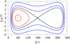 |
Fig. 1. Phase space of Eq. (12). The black line represents the separatrix between tadpole orbits (3 examples in red) and horseshoe orbits (in blue). The phase space is symmetric with respect to ζ = 180°. |
Out of the four fixed points of Eq. (12), the collision (ζ = 0°) is not in the validity domain of the equation and will be ignored. ζ = 180° is the hyperbolic (unstable) L3 Lagrangian equilibrium, while ζ = ±60° are elliptic (stable) configurations, the L4 and L5 Lagrangian equilibria. Orbits that librate around these elliptic equilibria are called tadpole, or trojan (in reference to Jupiter’s trojan swarms). Examples of trojan orbits are shown in red in Fig. 1. The separatrix emanating from L3 (black curve) delimits trojan orbits from horseshoe orbits (examples are shown in blue), for which the system undergoes large librations that encompasses L3, L4 and L5.
As previously stated, the libration of the resonant angle ζ is slow with respect to the average mean-motion η. The fundamental libration frequency ν is proportional to  . In the neighbourhood of the L4/L5 equilibria (Charlier 1906):
2.3. Dynamics in the eccentric and inclined directions
In order to study the co-orbital dynamics for low eccentricities and inclinations, ℋP can be expanded in Taylor series in the neighbourhood of (x1,x2,y1,y2) = (0,0,0,0), at 2nd order in xj, yj. This expansion can be written as (Laskar 1989; Robutel & Pousse 2013):
where  is given in Appendix A, and
  and
and  are sums of quadratic monomials in (xj,
 ) and (yj,
 ), respectively.
From this form we learn two things: at low eccentricity and inclination, the dynamics of the variables x = (x1, x2) and y = (y1, y2) are decoupled, and the dynamics of the variables ζ and Z are independent of xj and yj at first order. In the conservative case, the variational equations of x and y are given by Robutel & Pousse (2013), Robutel et al. (2015):

with
where Ax, Bx, Ay, By are complex-valued functions of ζ and are given in Appendix A.  represents the complex conjugate of B.
2.3.1. The eccentric direction
The dynamics in the direction of the eccentricities is given by the system (15). Although the coefficients of the matrix Mx are functions of the resonant angle ζ, ζ does not depend on the eccentricities at first order. One can hence evaluate Mx at a fixed point of the (ζ,Z) variables (L4 will be described here, results are equivalent for L5), and study the dynamics of the xj variable in the neighbourhood of the L4 circular equilibria. The eigenvector of the matrix Mx(L4) gives the direction of two remarkable families of quasi-periodic orbits that are represented in Fig. 2 (Giuppone et al. 2010; Robutel & Pousse 2013):
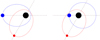 |
Fig. 2. Left: eccentric Lagrangian equilibrium: e1 = e2, ϖ1 − ϖ2 = ζ = ±60° and right: anti-Lagrangian equilibrium. At first order in the eccentricities: m1e1 = m2e2, ϖ1 − ϖ2 = ζ + 180°. |
-
The first eigenvector, paired with a null eigenvalue g− = 0, is tangent to the eccentric Lagrangian family (EL4), for which e1 = e2 and Δϖ = ϖ1 − ϖ2 = ζ.
-
The second eigenvector, paired with the eigenvalue g+ = 27/8(m1 + m2)/m0η, is tangent to the anti-Lagrangian family (AL4). For low eccentricities, this family is tangent to m1e1 = m2e2 and Δϖ = ϖ1 − ϖ2 = ζ + π.
Description of the dynamics at larger eccentricities can be found for example in Nesvorný et al. (2002), Giuppone et al. (2010), and Leleu et al. (2018).
2.3.2. The inclined direction
The dynamics in the direction of inclination is given by the system (15). In opposition to the eccentric direction, we do not learn anything by evaluating My at the L4 equilibria since all of its coefficients vanish for ζ = 60°. However, since the evolution of ζ is fast with respect to the secular evolution on the yj variables, we can obtain an approximation of the secular dynamics in the direction of the inclination for a given trajectory by averaging the expression of this system over a period 2π/ν with respect to the time t.
We note that Im(By(ζ)) = −Ay(ζ) (see Appendix A). In addition, the real part of By(ζ) is proportional to the expression of  (Eq. (12)), which is the derivative of a periodic function of period 2π/ν. Its average value over 2π/ν is hence null. As a result, the averaged My can be written:
where  is the averaged value of Ay(ζ) over a period 2π/ν, see Fig. 3. At ζ0 = 60° (Lagrangian equilibrium),
  and the system is degenerate. If
  , we identify the two eigenvectors:
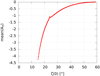 |
Fig. 3. Evolution of |

-
The first eigenvector, paired with a null eigenvalue s− = 0, is tangent to the direction I2 = I1 and Ω2 = Ω1: the two planets orbit in the same plane, inclined by I1 = I2 with respect to the reference frame.
-
The second eigenvector, paired with the eigenvalue
 , is tangent to the direction m1I1 = m2I2 and Ω2 = Ω1 + π: the inclination of both co-orbitals is constant and their lines of nodes slowly precess at the frequency s+.
We note that in the second direction the Oxy plane of the reference frame is perpendicular to the total angular momentum of the system (i.e. the Oxy plane is the invariant plane).
3. Stability of the Lagrangian equilibria L4 and L5 under external forces and mass change – the coplanar circular case
In this section we study the stability of the Lagrangian equilibria in the coplanar circular case under a generic dissipation, modelled by forces F1 and F2 applied on each planet. We assume that these forces are small with respect to the attraction by the central star. Using Gauss’ equations, the Poincaré variables are modified in the following way:
Where Fr, j is the radial force applied on the planet j, while Γj is the torque induced by the tangential force Ft, j. If the forces vary significantly over the orbital time-scale, they will also excite the eccentricities of the planets. For this work, we assume that variation of these forces over an orbital period is negligible, and that non-axisymmetric dissipative forces applied on the planets can be parametrised by Λ1, Λ2, and ζ = λ1 − λ2.
3.1. Model of the 1:1 MMR under dissipation and mass change
We start by developing an analytical model for the dynamics of the co-orbital configuration in the neighbourhood of the Lagrangian equilibria L4 and L5 in the dissipative case. To develop this model, we head back to the Hamiltonian transformations that we described in Sect. 2: we rewrite the equation of variation using the canonical variables Λj, λj. The equations of motion are given by the equation canonically associated with the Hamiltonian H, Eq. (2), to which we add the effect of the dissipation (Eq. (18)), and a slow, isotropic mass change for the planets parametrised by two constants ṁ1 and ṁ2.
We then perform a change of variables to uncouple the fast (i.e. associated to the mean motion) and semi-fast (i.e. resonant) degrees of freedom (Robutel et al. 2015):
It should be noted that this change of co-ordinates is canonical in the conservative case, here we need to add the terms relative to the dissipative forces and mass changes. Averaging over the fast angle φ, we obtain the following system:
with f a polynomial function of  and L, with trigonometric terms in ζ, and
  . Γj and Rj remain unchanged as we neglected their evolution over an orbital period. For the rest of this study, we focus on the evolution of the resonant degree of freedom (
 ,ζ).
,ζ).
3.2. Constant torques, radial forces and masses
At first we only consider the constant part of the torques and radial forces, Γj0 and Rj0, and constant masses (ṁj = 0). In this case, the evolution of the resonant degree of freedom ( ,ζ) is given by the equations associated to the following Hamiltonian:
where F(ζ) = cosζ − (2 − 2cosζ)−1/2,
and
3.2.1. Asymmetry of the phase space
In the restricted case (m1 ≪ m0, m2 = 0), the application of a constant torque on the co-orbitals result in a distortion of the phase space (Murray 1994; Sicardy & Dubois 2003). For a negative torque applied on the massive planet, it leads to a smaller tadpole domain for trailing massless particles than for leading ones, as the hyperbolic Lagrangian point L3 gets closer to L5, and further away from L4. We study here the displacement of the perturbed circular coplanar Lagrangian equilibria for two massive bodies, as a function of the dimensionless quantity CΓ, equivalent to the variable “α” in Sicardy & Dubois (2003). The position of these equilibria are obtained by solving the system:
For small enough dissipative forces (CΓ ≪ 1), we can compute analytically the positions of the new equilibria in the neighbourhood of their position in the absence of dissipation, ζ = π/3, and  . In order to keep track of the relative size of the terms in Eq. (20), we introduce the small dimensionless tracer ε. We make the assumption that the perturbative terms CΓ and
  are of similar size with mj/m0, traced by ε. ε is just a tool to neglect second-order perturbative terms, and we can later take ε = 1 for numerical estimation of the variables. Using the implicit function theorem, we look for a shift of size ε in the value of ζ and
  with respect to the non-dissipative case. We hence replace
  by
by  and ζ by π/3 + εz in the system (24), and solve it. At lowest order in ε, the new L4 equilibrium is located at:
Similarly, we compute the evolution of the position of the L3 equilibria by developing the system (24) in the neighbourhood of Δ = 0 and z = ζ − π = 0. Under the effect of the dissipative terms, the fixed point L3 is shifted by:
We hence have:
As a result, L3 and L4 get closer if  . If for example the torque per mass unit of the leading planet is lower that the torque per mass unit of the trailing planet, this results in a smaller trojan domain for the studied configuration.
For larger CΓ, we solve the system (24) numerically. This system has three solutions for ζ ∈ [0 ° ,360 ° ] as long as |CΓ|≲0.72. For larger absolute values of CΓ, two of the three roots merge and vanish. The positions of the equilibria are shown in Fig. 4. For these 3 equilibria, the value of  remain
  . We also compute, for this value of
  , the position of the separatrix emanating from L3. To do so, we find the solutions of the equation
  . The two separatrices were added as dashed lines to Fig. 4, and illustrate clearly the variation of the width of the trojan domain in the direction of ζ as a function of CΓ, as the orbits librating around L4 (resp. L5) have to remain between the dashed and solid black lines. These results are in agreement with those of Sicardy & Dubois (2003), and generalise them to the case of two massive bodies.
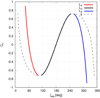 |
Fig. 4. Evolution of the position of L4, L3, L5, and the separatrix emanating from L3, in the direction of ζ with respect to CΓ, for |

3.2.2. Stability of the Lagrangian equilibria
We head back to small perturbations (CΓ ≪ 1,  ). The torques applied on each planet slowly change the total angular momentum of the system. Here we describe how the evolution of L changes the orbit of the co-orbitals on a long time-scale with respect to the resonant motion.
Let us consider a pair of co-orbitals on a trajectory librating in the neighbourhood of the L4 equilibria. We use z = ζ − ζL4 and  to describe the trajectory. On the resonant time-scale, this trajectory follow a level curve of the Hamiltonian (21). This level curve ℒ can be parametrised by zℒ > 0, with the energy of the curve being Hr(Δeq, ζL4 + zℒ). For zℒ = 0, ℒ(zℒ) goes through
  , estimated by solving
  . We obtain:
where
As L slowly evolves, so does W and Hr, and hence the level curve followed by the trajectory. However, the area enclosed by this level curve is an adiabatic invariant (Henrard 1982). As a result, a slow decrease of W leads the trajectory to follow level curves of larger and larger zℒ, while  decreases, see the left panel of Fig. 5 for an example. We hence need to give a more precise definition of the stability we want to consider. As the position of the fixed points and separatrix are scale-free in the ζ direction, see Fig. 4, we consider a trajectory to be converging toward the Lagrangian equilibria if zℒ decreases, as the trajectory is getting further away from the boundary of the tadpole orbits.
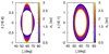 |
Fig. 5. Evolution of a trajectory in the ( |

We hence normalise the variable  by W, and call this new variable Δ:

By doing so, we lose the Hamiltonian formulation of the problem as we introduce a dissipative term in the equations of variation, but we explicit the effect of the change of total angular momentum on the newly-defined stability of the system: despite the small dissipative term, on the resonant time-scale a trajectory will remain close to a level curve of the Hamiltonian part of the system. For these new level curves, Δℒ only depends on zℒ. In these new variables, the stability is hence defined as a convergence toward L4 in both the ζ and Δ directions, while divergence from L4 happens in both ζ and Δ directions as well, as we can see in the right panel of Fig. 5. The evolution of Δ is given by:
where
where Ẇc is the term of Ẇ coming from the constant torques applied on the planets. The resonant part of the system of equations of variation (20) becomes:
As this is our main set of variables, we give the expression of the variable Δ with respect to the orbital elements:
while reciprocally, the circular angular momentum of each planet reads:
We now (and for the rest of this paper) study the stability of the new L4 equilibria (ζ ∈ [0, 180 ° ]), while the stability of L5 can be studied by swapping the indices of the planets. The L4 equilibria is located in:
To do so, we linearise the resonant part of the system (20) in the neighbourhood of ΔL4 and ζL4:
where Δ′=Δ − ΔL4, z′ = z − zL4, and J4 is the Jacobian matrix of the system (20) computed at the equilibrium (36). We make a final change of coordinates that diagonalises the system (37). In this new set of variables (z1,z2), the equations of variation reads:
where:
and
We hence obtain a modification of the classical resonant frequency ν0 in the neighbourhood of L4 (39), plus a hyperbolic term given in (40). As uc and ν are not constant due to the evolution of the masses and the total angular momentum L, we will study the stability of “partial” equilibria (see for example Vorotnikov 2002) by dividing the variables into two groups: the variables with respect to which the stability is investigated (Δ,ζ), and the remaining variables L, m1 and m2. The linearised system with a diagonal matrix Eq. (38) allows for a trivial application of results on the stability of the partial equilibrium z1 = z2 = 0 (see Appendix B): The partial equilibrium (36) is stable if uc is negative or null. From now on, we also make the assumption that a positive value induces a divergence from this equilibrium.
As previously stated, Ẇc/W represents the change of the size of the resonance as L evolves. If Ẇc/W < 0, the width of the resonance in the previous variable  is decreasing, leading to a slow increase of zl to retain a constant area enclosed by the level curve of the trajectory. As the system increases its amplitude of libration of the resonant angle, and gets closer to the separatrix of the tadpole domain, we consider the system to be diverging from the equilibrium. Looking at the expression of Ẇc/W, Eq. (32), it appears explicitly that inward migration (negative torques) have a destabilising effect on the co-orbital resonance, while outward migration tends to stabilise it.
3.3. Stability criteria for the Lagrangian configuration L4 under non-constant forces and mass change
In this section we study the stability of the Lagrangian equilibria L4 assuming that the variation of the dissipative forces can be parametrised by ζ and Δ, and that other variations are slow enough to be considered as constant with respect to the resonant time-scale. We also consider a slow, isotropic mass change for both masses. As in Sect. 3.2, we make the assumption that the perturbative terms CΓ,  and
and  are of similar size with mj/m0, traced by ε. As we did in the previous section, we normalise
  by W. As we now consider ṁj ≠ 0, we have:
The equations of variations (20) becomes:
For the variables  , ζ. Then we linearise these perturbations in the neighbourhood of (ΔL4,ζL4) by using the reduced variables Δ′=Δ − ΔL4, z = ζ − ζL4. Γj and Rj become:
where ΓjΔ = ∂Γj/∂Δ′, Γjζ = ∂Γj/∂z, and similar expressions for Rj. Despite the addition of these new terms in the equations of variation, the dominant terms of ΔL4 and ζL4 remains those computed in the case of constant forces, given in (36).
We hence linearise the rest of the system (42) in the neighbourhood of (ΔL4,ζL4), modelling the dissipative forces by the expression (43). Then, as in Sect. 3.2.2, we diagonalise the linearised system. Since the masses are not constant in this section, this transformation adds additional terms proportional to ṁ1 and ṁ2. However, as these terms are of size 𝒪(ε3), we can neglect them when we compute the eigenvalues of the linearised system. The dominant terms of the imaginary part remain:
However, the real part of the eigenvalue gets new terms:
![$$ \begin{aligned} 2u&=\varepsilon ^2 \left[ R_{1 \zeta } - R_{2 \zeta } + \frac{ m_2 \Gamma _{1\Delta } - m_1 \Gamma _{2\Delta } }{(m_1+m_2)W} \right.\nonumber \\&\quad \left. -\frac{\Gamma _{01}+\Gamma _{02}}{W} -\frac{1}{2} \frac{\dot{m}_1 + \dot{m}_2}{m_1+m_2} \right] . \end{aligned} $$](/articles/aa/full_html/2019/11/aa34486-18/aa34486-18-eq99.gif)
We hence obtain a small modification of the classical resonant frequency ν0 in the neighbourhood of L4 (44), plus a hyperbolic term given in Eq. (45). We note that at lowest order in ε the equilibrium point remains elliptic because of our assumptions on the relative size of the dissipative terms with respect to mj/m0. As in Sect. 3.2.2, we can deduce the stability of the system by estimating the sign of u: a negative value of u induces a convergence of the system toward the exact resonance, while a positive value led to a divergence.
The term-by-term physical interpretation of this criterion (the sign of u, Eq. (45)) is straightforward: if for example R1ζ is the only non-zero term of u and using Eqs. (18) and (43), we have:

If R1ζ < 0, z converges toward 0, hence ζ converges toward ζL4. Similarly, a negative Γ1Δ implies that the planet “1” migrates inward faster when Δ > 0 (i.e. when a1 > a2), which also pushes the planet towards the exact resonance.
The terms in Γj0 and ṁj were already described in the previous section, and take into account the evolution of the width of the resonance as the masses and total angular momentum of the configuration slowly evolve.
In the following sections, we apply the stability criterion u in the case of planets evolving in a protoplanetary disc.
4. Axi-symmetric dissipative forces: 1D protoplanetary discs
Gravitational interactions between the planets and their parent disc impact on the planets’ orbital parameters, typically causing them to migrate, either inwards towards the star or outwards away from the star (Goldreich & Tremaine 1979; Artymowicz 1993; Papaloizou & Larwood 2000). Planet eccentricities and inclinations are also affected by the interactions with the disc, typically causing them to be damped, forcing the planets to orbit their parent star on coplanar circular orbits (Cresswell & Nelson 2006; Bitsch & Kley 2010). The orbital evolution of the planets is the result of various torque components from the disc acting on them, such as the Lindblad torque, corotation torque, and horseshoe drag (Baruteau et al. 2014). For a single planet in a protoplanetary disc, two regimes are usually considered: As long as a planet is not massive enough to perturb the disc considerably, the planet is called to be in type I migration. As it is growing, it starts to open a gap around its orbit, and once this gap is deep enough, it migrates in type II regime. In this section, we assume that the perturbation of the disc by each planet is negligible, and hence that usual type I migration formulae can be applied on each planet individually.
We also assume that the unperturbed disc is axi-symmetric, and we study the stability of the coplanar circular co-orbital resonance in this case. Under this assumption, only the tangential forces (or torque) will play a role in the stability of the configuration (see the expression of the criterion u, Eq. (45)). In the literature, these torques are often modelled by migration time-scales τaj, used as prescriptions for the evolution of the semi-major axes:  , which implies a dissipative term for the evolution of the angular momentum of the planet of the form:
  .
.
4.1. Analytic model of type 1 migration
Tanaka et al. (2002) and Tanaka & Ward (2004) derived a linear model of the wave excitation in three-dimensional isothermal discs to obtain an analytical model for the torques induced by the Lindblad and corotation resonances. Following their notation, we consider a gaseous disc parametrised by its aspect ratio h and its surface density Σ(r), such that:
where H is the scale height, h0 is the aspect ratio at 1 au and f is the flaring index, and

where Σ0 is the surface density at 1 au and α parametrises the slope of the surface density. At first order in the inclination and eccentricity, we have:
for the evolution of the semi-major axis (Tanaka et al. 2002), with
where  is the Keplerian angular velocity of the planet. Considering Eqs. (47) and (48), and neglecting the effect of the eccentricity on the star-planet distance, τ reads:
At this stage, it becomes clear that taking τaj as a constant is a strong assumption that would force the semi-major axis to behave as an exponential decay. We hence introduce the variable Kj that parametrises the local slope of the migration:

The effect of the disc on the angular momentum of each planet is hence given by:
Expanding the torque applied on each planet at first order in Δ,  , we have:
and:
The effect of dissipative forces modelled by τaj (Eq. (52)) on the co-orbital configuration can be deduced from the expressions (54) and (55) and the criterion u, Eq. (45). The Lagrangian point is attractive if:

Figure 6 represents the K values for which the equilibrium becomes repulsive (above the line of a given mass ratio) as a function of τ1/τ2 ≈ τa1/τa2, in the special case K = K1 = K2. These results apply to the neighbourhood of the L4 or L5 equilibria, hence to tadpole orbits with small amplitudes of libration, as they were derived from the linearisation of the system (42) in the neighbourhood of L4. We then check the validity of this criterion for different amplitudes of libration in the case m1 = 10m2. We integrate the equations of the 3-body problem using the variable-step integrator DOPRI (Dormand & Prince 1980). In addition, the migration of the semi-major axis is modelled using
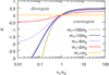 |
Fig. 6. Attraction criterion for the L4 and L5 equilibria in the dissipative case, for different values of m2/m1. The equilibria are attractive if K is below the curve, and repulsive if K is above. The grey squares represent the attraction limit for a horseshoe orbit and were derived numerically, see the text for more details. |
where rj is the position of the planet j with respect to the star. The tests were made using m0 = 1, m1 = 5 × 10⁻⁵, m2 = 5 × 10⁻⁶, taking as initial conditions ej = Ij = 0, a1 = a2 = 1 au and ζ0 = 58°, 50°, 40°, 30° and 20°. For each initial value of ζ, a grid of cases were integrated for different values of K and τw1/τw2, using τw1 = 1/m1. The grey squares in Fig. 6 represent the threshold values of K for which the configurations change from converging (below the curve) to diverging (above it) for ζ0 = 20° (horseshoe configuration). All other initial amplitudes of libration (initial values of ζ0) gave very similar results. It implies that, at least for the chosen masses, the attraction of the exact resonance does not depend significantly on the amplitude of libration in the case of axi-symmetric dissipative forces.
In the case of the torque from Tanaka et al. (2002), we have
Which hence verifies the relation K1 = K2 = α + 2f − 1/2, in addition to τa1/τa2 = m2/m1. Applying these additional constraints, the stability of the Lagrangian points depends only on m2/m1 and the parameter K. The critical value for K is thus:
which is represented in Fig. 7.
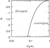 |
Fig. 7. Stability threshold for the L4/L5 equilibria when the torque induced by the protoplanetary disc is modelled using Eq. (49). The configuration diverge when K is above the line and converge when it is below. |
4.2. Stability in an evolving protoplanetary disc
The section above describes the evolution of the co-orbital resonance in a static environment, where the migration time-scales and disc parameters are assumed to be constant. However, protoplanetary discs do not remain static, so therefore it is important to determine how the co-orbital resonance evolves in a more global, ever-changing environment. Thus we now examine the behaviour of the resonance as the protoplanetary disc evolves on Myr time-scales, and also as a planet migrates from one region of a disc to another where the value of K can differ significantly. We use the disc model presented in Coleman & Nelson (2016b), where the standard diffusion equation for a 1D viscous α-disc model is solved (Shakura & Sunyaev 1973). Temperatures are calculated by balancing viscous heating and stellar irradiation against blackbody cooling. We use the torque formulae from Paardekooper et al. (2010, 2011) to calculate type I migration rates due to Lindblad and corotation torques acting on a planet. The Lindblad torque emerges when an embedded planet perturbs the local disc material, forming spiral density waves that are launched at the Lindblad resonances in the disc. Corotation torques arise from both local entropy and vortensity gradients in the disc, and their possible saturation is included in these simulations. The influence of eccentricity and inclination on the migration torques and the damping of eccentricities and inclinations are also included (Cresswell & Nelson 2008; Fendyke & Nelson 2014). These torques exchange angular momentum between the planet and the gas disc, and depending on their strength and direction can result in a torque being exerted on the planet, either inwards or outwards.
Figure 8 shows the gas surface density (left panel), disc aspect ratio h (middle panel) and the calculated value for K (right panel) at 4 different times throughout the disc lifetime. The blue line shows the profiles at the beginning of the disc lifetime, with the red, yellow and purple lines showing the profiles at 1, 2 and 3 Myr respectively. The disc lifetime here was ∼3.6 Myr. K = α + 2f − 1/2, as defined in Sect. 4.1.
 |
Fig. 8. Gas surface densities (left panel), disc aspect ratios (middle panel) and K (right panel) at t = 0 Myr (blue lines), 1 Myr (red lines), 2 Myr (yellow lines) and 3 Myr (purple lines) for a typical protoplanetary disc model. |
We then examine the evolution of a pair of co-orbital planets that are undergoing type I migration in the protoplanetary disc represented in Fig. 8. The masses of the planets are 10 and 5 M⊕ for the primary and secondary respectively, giving a mass ratio of 2. The top panel of Fig. 9 shows the evolution of semimajor axis as the planets migrate through the disc, showing that they remain in co-orbital resonance, even when migrating from 10 au down to the inner edge of the disc. The bottom panel shows the values for the surface density gradient α (blue line), the aspect ratio gradient f (red line), and the corresponding value of K (yellow line) at the planet’s location. As the planets originate in the outer irradiation dominated region of the disc, K has a value ∼1.75. But as the planets migrate in closer to the central star, they enter the viscous dominated region of the disc where the transition in opacities significantly impacts α and f, causing K to drop to below 0 for a time before rising back to just above 0. As the planets near the inner edge of the disc, K settles to just below 0. Whilst the planets are migrating through the different regions of the disc, they will either be converging towards the resonance or diverging away from the resonance, depending on the local disc conditions. Figure 10 shows the amplitude of libration (top panel) and the corresponding K′=K − K0 for the two migrating planets in Fig. 9.4pt
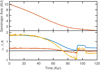 |
Fig. 9. Top panel: temporal evolution of semimajor axis for a pair of co-orbital planets. Bottom panel: surface density index α (blue line), aspect ratio index f (red line), and corresponding K (yellow line) at the planets’ location over time. |
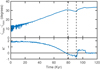 |
Fig. 10. ζmax − ζmin and K′ over time. When K′ is positive, resonance is diverging, and when K′ is negative, the resonance is converging. The dashed lines show there K′ changes sign, indicating the change from convergence to divergence or vice versa. |
When looking at Fig. 10, it can be seen that the amplitude of libration is increasing at the start of the simulation whilst K′∼2. As the planets migrate into the inner regions of the disc, K′ drops to begin fluctuating around 0. The first dashed line shows where the amplitude of libration begins to converge, and this lines up just after K′ reaches negative values. This is expected from the analytical model in Sect. 4.1. However, the analytical model uses the simplified type I migration torque formulae from Tanaka et al. (2002), whereas the evolving disc model here uses torque formulae from Paardekooper et al. (2010, 2011) that includes a more accurate treatment of the corotation torque. Despite these differences, it is interesting to see that the behaviour of the co-orbital resonance roughly matches what is expected from the Tanaka formulae, i.e. converging when K′ is negative and diverging when K′ is positive.
The planets migrating in Figs. 9 and 10 migrated until they reached the disc inner edge, close to the central star. Whilst doing so, they moved away from the co-orbital resonance, eventually breaking out of the resonance. However global simulations of planet formation have shown that planets in co-orbital configurations cover a wide range of semimajor axes at the end of the disc lifetime (Coleman & Nelson 2016a,b).
We now consider the case where the mass of a planet in the co-orbital resonance is changing over time in addition to its migration in the disc, meaning that it is accreting gas or planetesimals. As show in Sect. 3.3, both slow mass accretion and migration in the disc changes the width of the resonance in the way that leads to a divergence from the equilibrium (if the size of the resonance decreases due to inward migration), or to a convergence towards it (mass accretion or outward migration).
Figure 11 shows the relative change in mass against the relative change in angular momentum for a number of evolving planets at different locations of the protoplanetary disc and of different masses. We note that these planets are not in co-orbital configuration but are used to probe the torque felt and their accretion rate during their evolution in the disc. The planets shown in Fig. 11 were placed in a nominal protoplanetary disc similar to those shown in Coleman & Nelson (2016b). The black line shows where the sum relative changes in mass and angular momentum equate to zero, indicating no change in the stability of the co-orbital resonance. Planets that are evolving above this line will be accreting mass at a faster rate than they are migrating inwards and as such will be introducing a stabilising effect to their co-orbital region. For planets evolving below the line, then the opposite will occur, and they will diverge from the equilibrium. It is interesting to note, but not shown in the figure, that if a planet is undergoing outward migration, then the co-orbital resonance will be always be stabilising, so long as the planet is not losing mass at a significant rate. Looking at the regimes that specific planets operate in, we see that when a planet is small and growing through planetesimal or pebble accretion (yellow line), it is typically above the black line, since the planet is increasing in mass faster than it is migrating, stabilising the co-orbital region. For more massive planets, of mass between 10–20 M⊕, that are accreting few pebbles and/or planetesimals, but are accreting gas slowly (red line), they will tend to sit below the black line, destabilising the resonance. This is due to them migrating faster than they are accreting, however this is also highly dependant on the local disc profiles, which could allow planets to become trapped and migrate inwards slowly, reducing the magnitude of the destabilisation. For example, the red line shows the evolution of a ∼15 M⊕ planet initially orbiting at 5 au. The location of the planet in the protoplanetary disc, will also affect how close they appear to the black line in Fig. 11, since the migration torques are dependant on the local disc conditions, for example the 15 M⊕ planet shown by the red line would be shifted to the right of the plot if it was initially orbiting at 20 au, instead of 5 au as is shown in the plot. For planets that grow into giant planets through runaway gas accretion (blue and purple lines), initially they are in a regime of significant stabilisation as they accrete gas extremely quickly. Once the runaway gas accretion phase ends, they accrete gas at a slower rate, but migrate at a similar rate, reducing the effects of the stabilisation, before ultimately making it destabilising. Again, given the location in the disc that these planets occupy, this will mainly affect the rate of change of angular momentum, possibly making the co-orbital region stabilise or destabilise at a faster rate. For the giant planet that survives migration (purple line), meaning it does not migrate into the central star, the period of slow type-II migration (at the bottom of Fig. 11) is destabilising for the co-orbital region. This is again due to the planet migrating at a faster relative rate than it is able to accrete gas.
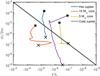 |
Fig. 11. Evolution of the relative change in mass against the relative change in angular momentum for four different planets over time. Black squares denote the starting point for the planets, whilst black crosses denote where the planets finish. Regions above the black line act to stabilise the co-orbital resonance, whilst below the line destabilises. |
Both mass accretion and migration hence have significant impacts on the evolution of the co-orbital resonance in the disc and have to be taken into account. In Sect. 5, we estimate how the perturbations of the disc induced by the pair of planets perturbs the torque that is applied to each of them.
4.3. Population outcome
While Sect. 4.2 examined the evolution of the co-orbital resonance in an evolving protoplanetary disc, it is interesting to see how often these co-orbital resonances actually occur in a much larger suite of simulations. To do this, we searched for co-orbital resonances in a recent population of simulations which studied planet formation around low mass stars. The simulations initially began with a realistic range of initial conditions, such as disc mass and solid mass, and used a similar disc model to that described in Sect. 4.2, but which had been adapted to being suitable for a low mass star (see Sect. 3 of Coleman et al. 2017). The main aim of these simulations was to examine the formation of planetary systems, through pebble or planetesimal accretion, around low-mass stars of mass 0.1 M⊙, similar to Trappist-1 and Proxima Centauri (Coleman et al. 2019). Initially in these simulations, a number of low mass planetary embryos (mp < 0.1 M⊕) would be scattered throughout the disc, and would be able to either accrete pebbles or planetesimals, and also undergo type I migration. As the planets migrate they become trapped in resonant chains, typically involving first-order resonances, but could also become trapped in co-orbital resonances. As the systems evolve, the planets migrate to their final locations, sometimes maintaining their resonant chains and also their co-orbital configurations. The planetary systems are integrated for 3–5 million years after disc dispersal to allow the planetary systems to continue to evolve in an undamped environment.
We analysed the outcome of the 880 systems generated in the pebble accretion scenario and found co-orbitals in ≈12% of the final systems. Figure 12 displays all of these co-orbitals as a function of their semi-major axis and amplitude of libration at the end of the simulation. As expected, co-orbitals that migrated on their own and survived until the end of the disc lifetime tend to have a large amplitude of libration. However, the subgroup of co-orbitals that were trapped into a resonant chain with other planets seemed to be able to migrate close to the inner edge of the disc while retaining a small amplitude of libration.
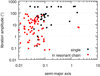 |
Fig. 12. Final amplitude of libration and semi-major axis of the co-orbitals formed in 880 synthetic systems around a 0.1 Solar mass star. 12% of the system had co-orbitals at the end of the run. Isolated co-orbital pairs are displayed in black, while those that are in resonance with another planet are displayed in red. Horseshoe configurations have an amplitude of libration above 180° degree. Other configurations are trojan. |
Indeed, we show in Appendix C that co-orbital configurations that would be unstable on their own can be stabilised during the protoplanetary disc phase by the presence of another planet trapped in first order mean motion resonances either inside, or outside, of the co-orbital pair.
5. Evolution in a protoplanetary disc: 2D hydrodynamical simulations
The torques applied on the planets in the previous sections were obtained for a single planet embedded in a disc. When there is more than one planet in the disc, the surface density perturbations by the other planets can alter the torque on each individual planet (Baruteau & Papaloizou 2013; Pierens & Raymond 2014; Brož et al. 2018). On the other hand, moderate-mass planets might open a partial gap around their orbits that can also vary the torque from its pure type-I value. In this section we take these effects into account by running two-dimensional (2D) locally isothermal hydrodynamical simulations using FARGO1 code (Masset 2000) for a system with two co-orbital planets in different mass regimes.
5.1. Disc and planets setups
The disc in our simulations is extended radially from 0.3 to 2.5 au and azimuthally over the whole 2π. It is gridded into Nr × Nϕ = 873 × 1326 cells with logarithmic radial segments. The resolution is chosen such that the half horseshoe width of a 3 M⊕ planet can be resolved by about 6 cells. The surface density profile is Σ = Σ0r−α = 2 × 10⁻⁴r−0.85 in code units. This corresponds to 1777 g cm−2 when the radial unit is 1 au and the mass unit is 1 M⊙. The disc viscosity follows the alpha prescription of viscosity νvisc = αvisccsH where cs is the sound speed and H is the disc scale height. These two quantities are related to the aspect ratio h as h = H/r = cs/vk, vk being the Keplerian velocity. The disc is flared with the aspect ratio of h = h0rf = 0.05r0.175. The reason of such choices for surface density and aspect ratio profiles will be explained in Sect. 5.2.
Planets are initiated radially at r1 = r2 = 1 au and azimuthally at λ1 = 0 (more massive one) and λ2 = +50 or −50 degrees. The mass of the planets are increased gradually during the first 50 years to avoid abrupt perturbations in the disc while they are kept on circular orbits until t = 100 yr. The total time of the simulations is 2000 or 3000 years depending on the migration rate of the planets. In cases that the planets migrate faster, we had to stop the simulations earlier to avoid the effect of the inner boundary. In order to have the consistency with the 1D simulations, we used ϵp = 0.4h for smoothing the planet’s potential. The planets do not accrete gas during these simulations and their masses stay constant after t = 50 yr.
We used various planet mass pairs as given in the left columns of Table 1, where m1 is the mass of the leading planet and m2 the mass of the trailing one. We saved the forces and torque on each planet 20 times per year, allowing us to estimate the value of the different terms of the stability criterion u, given by Eq. (45). The method to compute these different terms is given in Appendix D. Columns 3–8 of Table 1 give the averaged values of each quantity over the whole simulation time, and the 9th column is the quantity 2u, the sum of these contributions.
Value of the different terms of the stability criterion u for different hydro simulations with identical initial conditions except for the masses of the co-orbitals, given in the first two columns.
5.2. Comparison of 1D to 2D discs
First, we compare the evolved disc in the hydro-models to our 1D discs. In Sect. 4.2, we saw that the criterion (56), based on the analytical torques from Tanaka et al. (2002), was a good approximation to estimate the stability of the system. This criterion is a function of the local flaring index and surface density slope f and α through the parameter K which parametrises the local slope of the torque felt by both planets. In all of the simulations presented in this section, the flaring index and initial surface density slopes are f = 0.175, α = 0.85 implying that the disc is viscously in equilibrium. These values correspond to K = 0.7, for which the co-orbital planets in type-I migration should always be diverging (see Fig. 7). In our hydrodynamical runs, we estimate Kj – the value of K which is felt by the jth planet – that can be linked to the quantities Γj0 and ΓjΔ by the following relation (see Eq. (55)):
The Kjs for the hydro simulations are hence computed and given in the last two columns of Table 1. It appears clearly that the local slope of the torque felt by each planet is different from what is expected from Tanaka et al. (2002). The upper block of the table (the first three rows) contains the models with low-mass planets such that they do not perturb the disc greatly. The maximum surface density perturbation δΣ/Σ0 in these models is only about 3%. Therefore the difference of Kj with respect to the pure type-I migration which is expected for this type of planet is due to the presence of the co-orbital companion. For the models in the second block of the table, δΣ/Σ0 is at most 35%. In these models, the torques are modified both by the presence of the other planet and the partial gap. Hence, the stability of co-orbitals is expected to be different from those obtained using a 1D disc model. However, we note that if one of the co-orbitals is significantly more massive than the other, the constant part of the torque that applies on it remains the same regardless of the position of the lower mass planet. For large mass discrepancies, the first two terms of u (Eq. (45)) might hence be properly estimated by the 1D model, see for example Fig. 11. However, hydrodynamical simulations are needed to estimates the ΓjΔ and Rjζ terms.
5.3. Low to moderate mass planets: Super-Earth to mini-Neptune
In this section we study the evolution of co-orbitals in the super-Earth to mini-Neptune mass regime which are the planets that do not open a full gap in the disc. For comparison with the stability criterion developed in Sect. 3.3 (attractive equilibrium for negative u, repulsive for positive u), we give in Table 1 the quantity d(ζmax − ζmin)/dt, averaged over the simulation time. For the first two blocks of the table, where the no-gap and partial-gap opening planets are listed, the stability of the Lagrangian equilibrium is indeed correctly predicted by the criterion u as it has the same sign as d(ζmax − ζmin)/dt. On these sets of simulations, we can see a trend that was already remarked by Pierens & Raymond (2014): a more massive leading planet (m1 > m2) tends to stabilise the co-orbital configuration, while if the more massive planet is trailing, the system slowly evolves away from the equilibrium.
To see how much the presence of the second planet can affect the torque, we present the torque analysis for the models (m1, m2) = (5, 3) M⊕ in Fig. 13. In panel a, we plot the scaled torque Γj/Γ0, with  , vs. distance from the planet’s orbit δr, which is scaled to the planet’s mutual Hill radius
 ![$ R_{\mathrm{H}} = \sqrt[3]{(m_{1}+m_{2})/3m_{0}} $](/articles/aa/full_html/2019/11/aa34486-18/aa34486-18-eq125.gif) . Γj/Γ0 is the torque that is exerted on the jth planet by the material within ±δr of the planet’s orbit. In this figure, we compare the torque on each planet in the co-orbital simulation with the corresponding single-planet model. The scaled torques on single planet models are almost identical as expected for type-I migration. The torque on the co-orbital 5 M⊕ follows the single planets up to about 5 RH. It means that the torque from the co-rotation region and the its own spiral in this area is identical to the single planet model. As we move further out, the torque levels up until 8 RH, decreases until 10 RH, and increases again until it reaches the value of the total torque (dotted line). The cause of this variation can be found in panel b, where the surface density perturbation is shown, and in panel c, in which we plot the torque from each location in the disc on the planet. In panel c, the solid line demonstrates the torque from the inner disc and the dashed line is the negative of the torque from the outer disc. The advantage of this plot is that it shows where the torque from the disc in the co-orbital model differs from the single one. We see in panel c that the torque from the inner and outer disc is identical until about 5 RH, where the positive torque from the inner disc increases in the co-orbital model. This area of the positive torque, marked by a red dot, corresponds to the area between the two inner arms of the planets. The presence of the second planet creates a slight depression in the surface density at the left side of the planet compared to the right. It makes the torque from this area more positive. As we move further the torque drops strongly due to the fact that we get close to the over-dense part of the second planet’s spiral arm which is located on the left side of the planet and exerts a negative torque on the 5 M⊕. Then, this over-dense arm moves to the right side of the planet and its effect turns to a positive torque. The sum of all these components which arise from the depletion between the planets’ arms and other planet’s spiral is responsible for the deviation of the torque from the single planet models. The torque on the 3 M⊕ is very similar except that the effect of the other planet is stronger due to its stronger arm (panel d): the diamond and square symbols mark the passage of the 5 M⊕ planet’s spiral arms by the azimuthal position of the 3 M⊕ planet.
. Γj/Γ0 is the torque that is exerted on the jth planet by the material within ±δr of the planet’s orbit. In this figure, we compare the torque on each planet in the co-orbital simulation with the corresponding single-planet model. The scaled torques on single planet models are almost identical as expected for type-I migration. The torque on the co-orbital 5 M⊕ follows the single planets up to about 5 RH. It means that the torque from the co-rotation region and the its own spiral in this area is identical to the single planet model. As we move further out, the torque levels up until 8 RH, decreases until 10 RH, and increases again until it reaches the value of the total torque (dotted line). The cause of this variation can be found in panel b, where the surface density perturbation is shown, and in panel c, in which we plot the torque from each location in the disc on the planet. In panel c, the solid line demonstrates the torque from the inner disc and the dashed line is the negative of the torque from the outer disc. The advantage of this plot is that it shows where the torque from the disc in the co-orbital model differs from the single one. We see in panel c that the torque from the inner and outer disc is identical until about 5 RH, where the positive torque from the inner disc increases in the co-orbital model. This area of the positive torque, marked by a red dot, corresponds to the area between the two inner arms of the planets. The presence of the second planet creates a slight depression in the surface density at the left side of the planet compared to the right. It makes the torque from this area more positive. As we move further the torque drops strongly due to the fact that we get close to the over-dense part of the second planet’s spiral arm which is located on the left side of the planet and exerts a negative torque on the 5 M⊕. Then, this over-dense arm moves to the right side of the planet and its effect turns to a positive torque. The sum of all these components which arise from the depletion between the planets’ arms and other planet’s spiral is responsible for the deviation of the torque from the single planet models. The torque on the 3 M⊕ is very similar except that the effect of the other planet is stronger due to its stronger arm (panel d): the diamond and square symbols mark the passage of the 5 M⊕ planet’s spiral arms by the azimuthal position of the 3 M⊕ planet.
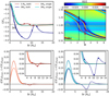 |
Fig. 13. Panel a: comparing the torque from the disc between a − δr and a + δr (solid lines) on m1 = 5 M⊕ planet (red lines) and m2 = 3 M⊕ (blue lines). The lighter colours represent the torques from the simulations with a single planet and the darker ones for the co-orbital simulation. The same colour dotted lines mark the torque from the whole disc. The y-axis is the scaled torque and x-axis the distance from the planets’ orbit in unit of their mutual Hill radius RH. Panel b: perturbed surface density. Two horizontal lines are drawn at 1 and 5RH from the planets’ orbits to guide the eye. Panel c: torque on m2 as a function of distance from the planet. Panel a is the cumulative torque but this panel and panel d show the torque only from the grid cells at a given distance from the planet. The dashed and solid lines belongs to the outer and inner disc, respectively. The colour code is the same as in panel a. To ease the comparison, we plot the negative of the torque from the outer disc. The symbols mark where the torque on the planets change due to the presence of the second planet. Panel d: same as panel c but for m1. |
As the spiral arms follow the planets in their libration around the Lagrangian equilibrium, both the torques and radial forces applied on each planet evolve over the libration time-scale, which is responsible for the non-negligible terms in Cols. 4, 5, 7, and 8 of Table 1.4pt
In Fig. 14, we present the same torque analysis for the model (m1, m2) = (6, 12) M⊕, which has two partial gap opening planets. As in the low-mass co-orbital model, the main cause of the deviation from the single-planet models is the depression of the surface density between the two planets’ arms and the presence of the other planet’s arm. In addition, the partial gap between the two planets (ϕ ∈ [π, 4π/3]) is deeper than the rest of the gap, which creates an additional offset for the torques applied on each planet.
The torques on the co-orbital planets is hence very different from those that would apply on a single planet, and the difference originates from the suppression of the surface density between the planets and the effect of the other planet’s spiral arm. According to our current knowledge, there is no extensive study that tell us how the depletion of mass between the co-orbitals changes by the disc parameters or the mass of the planets. On the other hand, the torque from the other planet’s spiral arm depends on the strength of the arm which depends on the planet’s mass, and opening angle of the spiral which is a function of the disc aspect ratio. Hence, we expect the stability of the co-orbitals depends on these two parameters because as the planets librate around their equilibrium point, their distance from each other and consequently from each other’s spiral would also change. In the following section, we remove the complexity of the partial gap and the co-rotation torque by replacing one of the co-orbitals with a gap-opening planet.
5.4. Gap-opening planets: A Jupiter and an Earth
In order to isolate the effect of the spiral arm of one planet on the other, we ran two simulations with a Jupiter-mass planet and an Earth-mass planet. In one of the simulations the Earth-mass planet is leading, and in the other it is trailing.
In Fig. 15 we present the disc surface density perturbation and the torque analysis for these models. The torque on the Earth-mass planet in these models only comes from the Jupiter-mass planet, either from the material accumulated in its Hill radius or spirals. As the upper panel of Fig. 15 shows, the spirals of the Earth-mass planet are so weak because there is little material in the gap in the disc to form them. The lower panel shows that the sign of the torque on the Earth-mass planet depends on its location compared to the Jupiter-mass planet. Here we explain the torque analysis for the planet on the right side (indicated by a cross sign) and the opposite argument is applied for the planet on the left (marked by a plus sign). Following the solid blue line in the lower panel, we see the (negative) torque slowly increases until the red line, where the gap edge is located. This indicates that the main torque (see the dashed blue line) does not come from the material around the Jupiter-mass planet. As we add the contribution of the material from the red to the yellow line, a large negative torque is exerted on the planet by the inner spiral which is located to the left side of the planet. As we get further, the continuation of the inner spiral adds a positive torque but since it is farther than the section on the left, it cannot change the torque considerably. The grey line marked where we reached the inner edge of the disc, and therefore, the oscillations after the grey line only originate from the outer disc.
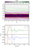 |
Fig. 15. Upper panel: perturbed surface density for the models with a Jupiter and an Earth. The location of the low-mass planets are marked with + and × signs. Because the surface density perturbation is identical in both cases, we only show the surface density map of one of them but marked the location of both planets for comparison. The red, yellow, magenta, and grey lines mark different distances from the planets’ orbit. The dashed lines belong to the model with the low-mass planet at × and the solid lines are for the one with planet at +. These lines are also added to the lower panel to denote the effect of the Jupiter’s spirals. Lower panel: same as panel a of Fig. 13. The green and blue curves show the torque on the low-mass planet initiated close to L4 and L5 equilibria, respectively. The scaling is the Jupiter’s Hill radius RH for the x-axis and Γ0 for the y-axis that is calculated using the Jupiter’s mass. |
Based on the calculations in Sect. 3.3, the partial derivatives ΓjΔ = ∂Γj/∂Δ and Rjζ = ∂Rj/∂(ζ − ζeq) are key parameters the for stability of the co-orbitals, see Cols. 4, 5, 7, and 8 of Table 1. Figure 16 represents the evolution over time of the torque and radial forces for the leading-Earth-mass planet case “×”. On the left panel, we can see that Γ1Δ > 0, which leads to a positive term in the expression of u hence destabilising the configuration. On the other hand, the left panel shows that R1ζ < 0, which induces a stabilising term. These two effects oppose one another and determine the attractiveness of the equilibrium. We note that in this particular case, our estimation of u did not match the evolution of the system: we computed a negative u, while the system is diverging from the equilibria. As the sum of the two dominant terms is an order of magnitude lower than each of these terms, this might be due to higher-order effects in the expansion of the torques and forces that were neglected when we computed the expression of u (in our runs, the semi-amplitude of libration is of ∼0.17 radians which is at the limit of the validity of the linear model).
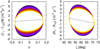 |
Fig. 16. Evolution of torque (left) and radial force (right) on the Earth-mass planet in the leading case “×”. The black lines show the linear approximation for the evolution of these quantities with respect to Δ and ζ − ζeq, respectively. |
The partial derivatives ΓjΔ and Rjζ applied on the Earth-mass planet come from the spiral arm of the Jupiter-mass planet, see Fig. 15. As these effects are of opposite sign for leading and trailing planets (bottom panel of Fig. 15), they lead to a qualitatively similar behaviour for the stability around the L4 and L5 equilibria of the giant planet. To confirm this trend, we ran a set of simulations with a 10 M⊕ planet either leading or trailing a Jupiter-mass planet for different disc parameters, varying the α parameter of the viscosity and the aspect ratio. Viscosity affects the gap depth and width, and the aspect ratio widens or tightens the spirals. For all the tested disc parameters, either both leading and trailing 10 M⊕ planets converged toward the equilibria, or they both diverged away from it.
In Fig. 17 we show the results for these 7 different disc profiles that we tested. Seemingly, the stability of the planets inside the gap of a massive planet is a delicate trade-off between the disc parameters, although based on this small set, lower viscosity and smaller aspect ratios (that result in deeper and wider gaps) seem to stabilise co-orbital configurations. As this dependency is key to estimating the probability of the existence of Earth to super-Earth mass trojan companions to giant planets, we will investigate this topic more thoroughly in a future study.
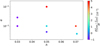 |
Fig. 17. Evolution of the libration angle for models with m1 = 10 M⊕, m2 = 1 MJup and in discs with different values for αν and aspect ratio h. |
6. Stability in the direction of the eccentricity and the inclinations
In this section we study the effect of dissipation on the evolution of the eccentricities and inclinations of the co-orbitals, for low values of ej and Ij (≲0.1). At first order, the Poincaré variables (Eq. (1)) read:
In the absence of dissipation, these variables follow the equations of variation given by the system (15).
We assume that the evolution of the orbital elements induced by dissipative forces can be modelled by migration and damping time-scales:

We note that modelling the migration by such a law is equivalent to taking K = 0 in Sect. 4.1. It can be shown that the results of this section remain valid for any value of K, as the local variations of the torques over the resonant time-scale have a negligible effect on the evolution of the variable xj and yj. We hence consider the following non-conservative terms:
for the evolution of the xj and yj. The equation of variations hence read:

where the Mx, My can be found in Appendix A,  and
and  (Eq. (63)). As we will be primarly interested in the evolution of the orbital elements ej and Ij, we normalise the variables xj:
  and
and  . The evolution of these new variables reads:
and the dissipative terms read:
6.1. Stability in the direction of the eccentricities
6.1.1. Constant masses
We study the stability in the direction xj, related to the eccentricity and the argument of periastron, in the neighbourhood of the L4 circular equilibrium for constant masses. In this section we consider dissipation time-scales that are not necessarily small with respect to  . The equation of variation of the variables xj is given by
where MX(L4) is obtained by estimating the terms of MX at the circular L4 equilibria, given by Eq. (25). The system of Eq. (65) have two eigenvalues. At first order in ε:
where
1/τX− = 1/τa− + 4/τe−, and
In the conservative case, 1/τe± = 1/τa± = zL4 = 0, and we obtain g− = 0 and g+ = i27/8(m1 + m2)/m0η. The direction associated to these eigenvalues were described in Sect. 2.3.1: the eccentric Lagrangian equilibrium, where e1 = e2 and ϖ1 − ϖ2 = ζ = ±π/3; and the anti-Lagrangian equilibrium, where m1e1 = m2e2 and ϖ1 − ϖ2 = ζ + π = ∓2π/3.
Figure 18 shows the values of τe2/τa1 for which the real component of the eigenvalues (68) vanishes, with respect to τa1/τa2. These plots were made using m1 = 10−4m0, τe1 = τe2m2/m1, and τa1 = 10/m1. For a given mass ratio, the manifold e1 = e2 = 0 is attractive below the two curves of the given colour. Above the solid line, the system diverges following the anti-Lagrangian direction; while systems above the dashed curve diverge following the eccentric Lagrangian direction. These curves were obtained using several assumptions on the relations between the masses and the damping and migration time-scales, and that the stability of the Xj directions in the τa1/τa2, τe2/τa1 plane depends greatly on these assumptions.
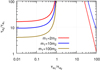 |
Fig. 18. Example of attraction criteria in the eccentric directions in the dissipative case, for different values of m2/m1. For this example, the relations m1 = 10−4m0, τe1 = τe2m2/m1, and τa1 = 10/m1 were chosen. Orbits in the neighbourhood of L4 will tend toward e1 = e2 = 0 if τe2/τa1 is chosen below both curves of a given colour. The solid lines represent the stability limit in the anti-Lagrangian direction, while the dashed one is the limit in the eccentric Lagrangian direction, see the text for more details. |
Figure 19 represents the evolution of two configurations taken on the left border of Fig. 18: τa1/τa2 = 0.01. In the left panel, τe2/τa1 = 5, while on the right τe2/τa1 = 20. The stability in the Xj directions is given by the position of the configurations relative to the blue curves of Fig. 18. In both cases, the motion relative to the direction of the eccentric Lagrangian equilibria (black solid lines in Fig. 19) is quickly damped as we are far below the dashed lines in both cases. As the quantity ϖ1 − ϖ2 converges toward 240 ° ( = ζ + 180°), which is the direction of the anti-Lagrangian equilibria, the eccentricity either decreases as this direction is stable (the left case is below the solid blue curve of Fig. 18), or increases if the anti-Lagrangian direction is unstable (the right case is above the solid blue curve).
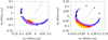 |
Fig. 19. Examples of the evolution of the quantities e2 and Δϖ for different initial conditions. The black dashed lines represent the direction of the anti-Lagrangian configuration while the black solid line is the direction of the Eccentric Lagragian equilibria. In both cases, the initial conditions are ω2 = ω1 + π, I1 = I2 = 0, m1 = 10m2 = 1 × 10⁻⁴m0, a1 = a2 = 1 au, e1 = 0.1, e2 = m1e1/m2 and ζ = 60°. Each trajectory is integrated for 20 Kyr, with the initial conditions represented by the black triangle, and the colour code representing the time (blue at t = 0, yellow at 20 Kyr). On the left panel, τe2/τa1 = 5, while on the rightτe2/τa1 = 20. In both cases, τa1/τa2 = 0.01. |
6.1.2. Effect of mass change
We now consider the effect of a slow, isotropic mass change on the eccentric Lagrangian equilibria and anti Lagrangian equilibria previously discussed. For this mass change to impact the evolution of the configuration, it has to be comparable to the migration and damping time-scales. We hence assume that the perturbative terms 1/τaj, 1/τej and ṁj/mj are of size ε2. The details of the computations can be found in Appendix E.
-
Evolution of the eccentricities along the anti-Lagrangian equilibria: taking 𝒳2 = 0, Eq. (E.5) yields, at second order in ε:
where
 is a positive real quantity and
 -
Evolution of the eccentricities along the eccentric-Lagrangian equilibria: taking 𝒳1 = 0, Eq. (E.5) yields, at second order in ε:
where
 is a positive real quantity.

If the eccentricities are damped by the disc (τej > 0) then the mode associated to the Eccentric Lagrangian equilibrium will always be damped toward e1 = e2 = 0. However the eccentricities can increase along the Anti-Lagrangian equilibria if the more massive of the two planets migrate inward (or accrete gas) fast enough (see Eq. (71)).
6.2. Stability in the direction of the inclinations
6.2.1. Constant masses
We study the stability in the direction Yj, related to the inclinations and the ascending nodes of the co-orbitals, for any amplitude of libration of the resonant angle. Eq. (A.2) becomes:
At first order in ε, MY(L4) can be diagonalised, with the diagonal elements being:
where
1/τX− = 1/τa− + 4/τI−, and
We note that the eigenvalues (75) have a similar expression to that in the direction of the eccentricity, Eq. (68), but here the results are valid for any amplitude of libration in the trojan and horseshoe domains. The amplitude of libration affects the stability in the Yj direction through the value of  (see Fig. 3).
The orbits can either be attracted toward I1 = I2 = 0, or diverge following m1I1 = m2I2 and Ω2 = Ω1 + π, or I2 = I1 and Ω2 = Ω1, see Sect. 2.3.2. Examples of convergence and divergence along m1I1 = m2I2, Ω2 = Ω1 + π are shown in Fig. 20.
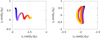 |
Fig. 20. Examples for the evolution of I2 and Ω1 − Ω2. In both cases, the initial conditions are Ω2 = Ω1 + π + 0.3, I2 = 2°, m1 = 10m2 = 1 × 10⁻⁴m0, a1 = a2 = 1 au, e1 = e2 = 0 and ζ = 60°. Each trajectory is integrated for 20 Kyr, with the initial conditions represented by the black triangle, and the colour code representing the time (blue at t = 0). In the left panel, τI2/τa1 = 1, while on the rightτI2/τa1 = 30. In both cases, τa1/τa2 = 0.01. |
6.2.2. Effect of mass change
We now consider the effect of a slow, isotropic mass change on the inclination of quasi-circular co-orbitals (up to first order in eccentricities). As we did for the study of the evolution of the eccentricities, we assume that the perturbative terms 1/τaj, 1/τIj and ṁj/mj are of size ε2, and that the mass evolution is isotropic. The details of the computations are identical to the eccentric case and can be found in Appendix E.
-
Evolution of the inclinations along m1I1 = m2I2, Ω2 = Ω1 + π: taking 𝒴2 = 0, we obtain, at second order in ε:
where
 is a positive real quantity and
 -
Evolution of the inclination along I1 = I2, Ω1 = Ω2: taking 𝒴1 = 0, we obtain, at second order in ε:
where
 is a positive real quantity.
If the inclination are damped by the disc (τIj > 0) then the mode associated to I1 = I2, Ω1 = Ω2 will always be damped toward I1 = I2 = 0. However the inclinations can increase along m1I1 = m2I2, Ω2 = Ω1 + π if the more massive of the two planets migrate inward (or accrete gas) fast enough (see Eq. (78)). We remind the reader that these results on the inclinations are valid for any amplitude of libration of the resonant angle, up to horseshoe orbits.
7. Summary and conclusions
7.1. Summary
In this paper we have studied the stability of the co-orbital resonance under dissipation in the planetary case ((m1, m2)≪m0). In Sect. 3 we developed an integrable model of the 1:1 MMR perturbed by a generic dissipation and derived the stability conditions of the L4 and L5 equilibria.
In Sect. 3.2 we showed that under the effect of a constant torque applied on each planet, the phase space of the resonance becomes asymmetric, as the position of the Lagrangian equilibria L3, L4 and L5 change. The tadpole (trojan) area is larger if the torque per mass unit applied on the leading planet is greater than the torque per mass unit applied on the trailing one. We also saw that if the difference between these two torques is too large, two out of the three equilibrium points could merge and vanish, leading to a phase space with a single equilibrium point. These results are in agreement with those of Sicardy & Dubois (2003), obtained in the restricted case (m1 ≪ m0, m2 = 0). This effect can also contribute to the instability observed by Pierens & Raymond (2014), where they showed that similar mass co-orbitals were unstable during the partial gap-opening regime, due to the opposite torques induced by a higher gas depletion between the two planet than everywhere else in the gap.
In Sects. 3.2.2 and 3.3, we then studied the stability of the Lagrangian equilibria L4 and L5 as a function of the forces applied on each planet, their masses mj, and the evolution of their mass ṁj. This study can be split into two parts:
-
First, the evolution of the masses of the co-orbitals, along with the constant torques that are applied on them, change the width of the co-orbital resonances. It can lead to either a convergence toward the Lagrangian equilibria in the case of outward migration (positive total torque, Γ10 + Γ20 > 0) or overall mass increase (ṁ1 + ṁ2 > 0), while inward migration (negative total torque) and mass loss induces a slow divergence from the Lagrangian equilibria. These results are in agreement with those of Fleming & Hamilton (2000), which were obtained in the restricted case (m1 ≪ m0, m2 = 0).
-
Second, if the forces applied on each planet vary over the resonant time-scale, we show that the dependency of the torques on the semi-major axis, and the dependency of the radial component of the perturbative forces on the value of the resonant angle, impact significantly the stability of the system (the effect of a radial dependency of the torque was discussed by Sicardy & Dubois 2003, in the restricted case).
These two effects were considered to derive the stability criterion u for the Lagrangian equilibria (Eq. (45)).
Sections 4 and 5 were dedicated to comparing these results to N-body simulations in 1D disc models, and hydrodynamic simulations. In Sect. 4, we applied type-I migration prescriptions on a pair of planets in an evolving protoplanetary disc. The stability criterion successfully predicts the stability of the system, as a function of their masses, their migration time-scale τaj, and the slope of that migration parametrised by Kj. In addition, running planetary system evolution through the disc lifetime allowed us to study the balance between the destabilising effect of inward migration and the stabilising effect of mass accretion: first, planets tend to grow in mass significantly faster than they migrate, which leads to a convergence toward the exact equilibrium. However, in the later stages of the disc lifetime, the planets migrate quickly, leading to a divergence from the equilibrium. In addition, we showed that co-orbitals that belong to a resonant chain with other planets can be stabilised during the migration phase.
However, the comparison to hydrodynamics simulations show the limits of the 1D models: despite having similar initial conditions for the disc, the forces that are applied on each planet in the hydrodynamical simulation are totally different from those given by type-I prescriptions. Indeed, as the two planets evolve around the same semi-major axis, the disc is significantly perturbed both radially and azimuthally (Fig. 13, see also Brož et al. 2018). It creates structures whose effects cannot be azimuthally averaged, as they follow the position of the planets. Notably, as both planets librate around the Lagrangian equilibria, they move relatively to one another’s spiral arms. The additional torques and radial forces applied on each planet hence evolve over the libration time-scale, that can either have a stabilising effect, or destabilising one, see Table 1. It is the sum of all these terms that dictates the evolution of the system.
In the super-Earth range (3–5 M⊕) we note a trend that was observed by Pierens & Raymond (2014): more massive leading planets tend to stabilise the system. We show here that this stabilisation is due to the variations of the torques felt by each planet over the resonant libration, as they are successively closer to, and then further away from, one another’s spiral arm. This trend is also present in the mini-Neptune regime (up to 15 M⊕) with the apparition of other structures, such as a partial gap that is deeper between the co-orbitals.
Finally, in the case where the gap is totally open, we ran a set of simulations with a Jupiter-mass planet trailed or preceded by Earth or super-Earth mass planets. Here the dominant effect for the stability was the variation of the radial forces and torques applied on the Earth-mass planet by the Jupiter-mass planet’s spiral arms, during each libration period. The symmetry of the spiral arms with respect to the Jupiter-mass planet led to a similar behaviour for leading and trailing smaller mass companions: for all tested disc profiles, both leading and trailing companions behaved in a similar way (both diverging from or both converging toward L4/L5). However, as shown in Fig. 17, different disc parameters change the stability of such configurations. The effect of the disc parameters on the shape and strength of the Jupiter-mass planet’s spiral arms will be the subject of a future study.
In Sect. 6, we studied the stability of the Lagrangian equilibrium in the direction of the eccentricities (at first order), and the stability of the whole tadpole and horseshoe domain in the direction of the inclinations (at first order as well). We have shown that even in the case were the dissipative forces tend to damp the eccentricities and inclination of the planets, those could increase along a particular family of orbits.
7.2. Conclusions
7.2.1. On the limitation of 1D disc models
We have shown that disc-planet coupling generates structures in the disc that cannot be azimuthally averaged, leading to variations over time of the torques and radial forces that applies on each planet. Using similar disc profiles in 1D and hydrodynamical simulations, these differences lead to opposite results on the stability of the Lagrangian equilibria. Similar observations were made by Brož et al. (2018) in a more general context.
7.2.2. On the evolution of co-orbitals
Trojan swarms. The asymmetry between the L4 and L5 domains induced by the difference of torque per mass unit (Fig. 4) can be used to explain the potential asymmetry between the leading and trailing Jupiter’s and Neptune’s trojan swarm However it requires one to properly estimate the torques that are felt by each of the asteroids: we showed in Sect. 5 that the torque per mass unit applied by the protoplanetary disc on the leading and trailing Trojans are not negligible, and comes mainly from the Jupiter-mass planet’s spiral arms (see Fig. 15). These torques will hence strongly depend on the disc parameters, and are of opposite sign for L4 and L5 Trojans. As a result, L4 and L5 domains would be more symmetric than if we apply the same torque on all asteroids.
Co-orbital exoplanets. We have shown that the attractiveness of the Lagrangian equilibria depends on the mass distribution between the planet, the total mass, the accretion rate, the constant torques and radial forces that apply on each planet, but also on how these quantities evolve on the resonant time-scale. We have shown that long inward migration destabilises co-orbitals, while outward migration and mass accretion tend to stabilise them. Figure 11 shows that the stabilising terms coming from mass accretion is comparable to the destabilising terms coming from inward migration, and hence both have to be taken into account to properly estimate the stability of a system. However, this stabilising effect comes into play mainly in the earlier phase of the planet’s evolution. While in the later stages, its evolution is dominated by the migration.
As in Pierens & Raymond (2014), we also found that leading massive trojans tend to stabilise the configuration. In their study, these authors also showed that equal mass co-orbitals can be disrupted during the gap opening stages. We have shown that the stability of Earth-mass planets as trojan companions of a Jupiter-mass planet depend on the disc parameters, but that both L4 and L5 configurations tend to be stable or unstable for a given set of disc parameters.
We have shown that unstable co-orbital configurations could be stabilised by being trapped in first order mean motion resonance with a third planet, although in this part of the study we neglected the perturbation coming from the different planet’s spiral arms (Brož et al. 2018).
It is worth noting that the Lagrangian equilibria being repulsive does not necessarily imply that no co-orbital configurations can remain, it only implies that the amplitude of libration around the Lagrangian equilibria slowly increases over the migration time-scale, although that can lead to trojan orbits becoming horseshoe orbits, or even exiting the resonance. Similarly, attractive Lagrangian equilibria only implies a slow convergence toward it, but the configuration can still be disrupted on shorter time-scales for example through N-body interaction with other planets (Robutel & Bodossian 2009; Leleu et al. 2019).
7.2.3. On the detectability of co-orbitals exoplanets
In our hydro-simulation runs, in the [3, 15] M⊕ range and for a given disc profile, all configurations with a leading more massive planet were attracted toward the Lagrangian equilibria for planets. On the contrary, for the Jupiter-mass planet’s Earth sized trojan the stability seemed to depend very little on who is leading in the orbit, but we showed that different disc parameters can change the attractiveness of the Lagrangian equilibria. In addition, Cresswell & Nelson (2009) found that during the co-orbital’s evolution in the disc, the mass discrepancy between the two planets keep increasing because the more massive planet starves-off the other.
Our study of the stability of the Lagrangian equilibria in the inclined direction also leads to important conclusions regarding the detectability of co-orbitals. We have shown that as long as the disc tend to damp inclinations, the system can evolve toward two directions: either coplanar co-orbitals, or mutually inclined co-orbitals following the m1I1 = m2I2, Ω1 = Ω2 + π direction. This later direction is favoured if the proper migration of the more massive of the two planets, or its mass accretion rate, is faster than the inclination damping of the smaller planet. As the inclination damping of the smaller planet is reduced by the deeper partial or full gap created by the more massive planet, that could significantly reduce the transit probability of both co-orbitals. Similarly, even when the disc damps the eccentricities of the two planets, these eccentricities can increase following the anti-Lagrangian equilibria m1e1 = m2e2ω1 − ω2 = ζ + π (Giuppone et al. 2010; Leleu et al. 2018).
Mutually inclined co-orbitals can still be detected using transit timing variations (TTVs; Ford & Holman 2007; Vokrouhlický & Nesvorný 2014; Leleu et al. 2019) or radial velocities (Laughlin & Chambers 2002; Leleu et al. 2015), however, these methods require that the co-orbitals librate with a significant amplitude around the Lagrangian equilibrium, and that the observations baseline is at least comparable with the libration time-scale. In addition, the planets have to be of comparable masses for the radial velocity method, as well as for TTVs if it is the larger of the two planets that is transiting. Finally, even in the absence of libration, the combination of transit and radial velocity measurements can be used to detect co-orbital configurations (Ford & Gaudi 2006; Leleu et al. 2017), although this requires good constraints on the eccentricity of the transiting planet.
Acknowledgments
The authors acknowledge support from the Swiss NCCR PlanetS and the Swiss National Science Foundation. S.Ataiee acknowledges the support of the DFG priority program SPP 1992 “Exploring the Diversity of Extrasolar Planets (KL 650/27-1)”.
References
- Artymowicz, P. 1993, ApJ, 419, 166 [NASA ADS] [CrossRef] [Google Scholar]
- Baruteau, C., Crida, A., Paardekooper, S.-J., et al. 2014, Protostars and Planets VI, 667 [Google Scholar]
- Baruteau, C., & Papaloizou, J. C. B. 2013, ApJ, 778, 7 [NASA ADS] [CrossRef] [Google Scholar]
- Beaugé, C., Sándor, Z., Érdi, B., & Süli, Á. 2007, A&A, 463, 359 [NASA ADS] [CrossRef] [EDP Sciences] [Google Scholar]
- Bitsch, B., & Kley, W. 2010, A&A, 523, A30 [NASA ADS] [CrossRef] [EDP Sciences] [Google Scholar]
- Brož, M., Chrenko, O., Nesvorný, D., & Lambrechts, M. 2018, A&A, 620, A157 [NASA ADS] [CrossRef] [EDP Sciences] [Google Scholar]
- Charlier, C. V. L. 1906, Astron. Nachr., 171, 213 [NASA ADS] [CrossRef] [Google Scholar]
- Coleman, G. A. L., & Nelson, R. P. 2016a, MNRAS, 460, 2779 [NASA ADS] [CrossRef] [Google Scholar]
- Coleman, G. A. L., & Nelson, R. P. 2016b, MNRAS, 457, 2480 [NASA ADS] [CrossRef] [Google Scholar]
- Coleman, G. A. L., Nelson, R. P., Paardekooper, S. J., et al. 2017, MNRAS, 467, 996 [NASA ADS] [CrossRef] [Google Scholar]
- Coleman, G. A. L., Leleu, A., Alibert, Y., & Benz, W. 2019, A&A, 631, A7 [NASA ADS] [CrossRef] [EDP Sciences] [Google Scholar]
- Cresswell, P., & Nelson, R. P. 2006, A&A, 450, 833 [NASA ADS] [CrossRef] [EDP Sciences] [Google Scholar]
- Cresswell, P., & Nelson, R. P. 2008, A&A, 482, 677 [NASA ADS] [CrossRef] [EDP Sciences] [Google Scholar]
- Cresswell, P., & Nelson, R. P. 2009, A&A, 493, 1141 [NASA ADS] [CrossRef] [EDP Sciences] [Google Scholar]
- Crida, A. 2009, ApJ, 698, 606 [NASA ADS] [CrossRef] [Google Scholar]
- Deck, K. M., Payne, M., & Holman, M. J. 2013, ApJ, 774, 129 [NASA ADS] [CrossRef] [Google Scholar]
- Dormand, J. R., & Prince, P. J. 1980, J. Comput. Appl. Math., 6, 19 [CrossRef] [MathSciNet] [Google Scholar]
- Érdi, B. 1977, Celest. Mech., 15, 367 [NASA ADS] [CrossRef] [Google Scholar]
- Fabrycky, D. C., Lissauer, J. J., Ragozzine, D., et al. 2014, ApJ, 790, 146 [NASA ADS] [CrossRef] [Google Scholar]
- Fendyke, S. M., & Nelson, R. P. 2014, MNRAS, 437, 96 [NASA ADS] [CrossRef] [Google Scholar]
- Fleming, H. J., & Hamilton, D. P. 2000, Icarus, 148, 479 [NASA ADS] [CrossRef] [Google Scholar]
- Ford, E. B., & Gaudi, B. S. 2006, ApJ, 652, L137 [NASA ADS] [CrossRef] [Google Scholar]
- Ford, E. B., & Holman, M. J. 2007, ApJ, 664, L51 [NASA ADS] [CrossRef] [Google Scholar]
- Giuppone, C. A., Beaugé, C., Michtchenko, T. A., & Ferraz-Mello, S. 2010, MNRAS, 407, 390 [NASA ADS] [CrossRef] [Google Scholar]
- Giuppone, C. A., Benitez-Llambay, P., & Beaugé, C. 2012, MNRAS, 421, 356 [NASA ADS] [Google Scholar]
- Goldreich, P., & Tremaine, S. 1979, ApJ, 233, 857 [NASA ADS] [CrossRef] [MathSciNet] [Google Scholar]
- Henrard, J. 1982, in NATO Advanced Science Institutes (ASI) Series C, ed. V. Szebehely, 82, 153 [Google Scholar]
- Janson, M. 2013, ApJ, 774, 156 [NASA ADS] [CrossRef] [Google Scholar]
- Laskar, J. 1989, Les variables de Poincaré et le développement de la fonction perturbatrice, Notes scientifiques et techniques du Bureau des Longitudes S026, Groupe de travail sur la lecture des Méthodes nouvelles de la Mécanique Céleste [Google Scholar]
- Laskar, J., & Robutel, P. 1995, Celest. Mech. Dyn. Astron., 62, 193 [NASA ADS] [CrossRef] [MathSciNet] [Google Scholar]
- Laughlin, G., & Chambers, J. E. 2002, AJ, 124, 592 [NASA ADS] [CrossRef] [Google Scholar]
- Lee, M. H., & Peale, S. J. 2002, ApJ, 567, 596 [NASA ADS] [CrossRef] [Google Scholar]
- Leleu, A., Robutel, P., & Correia, A. C. M. 2015, A&A, 581, A128 [NASA ADS] [CrossRef] [EDP Sciences] [Google Scholar]
- Leleu, A., Robutel, P., Correia, A. C. M., & Lillo-Box, J. 2017, A&A, 599, L7 [Google Scholar]
- Leleu, A., Robutel, P., & Correia, A. C. M. 2018, Celest. Mech. Dyn. Astron., 130, 24 [NASA ADS] [CrossRef] [Google Scholar]
- Leleu, A., Lillo-Box, J., Sestovic, M., et al. 2019, A&A, 624, A46 [NASA ADS] [CrossRef] [EDP Sciences] [Google Scholar]
- Lillo-Box, J., Barrado, D., Figueira, P., et al. 2018a, A&A, 609, A96 [NASA ADS] [CrossRef] [EDP Sciences] [Google Scholar]
- Lillo-Box, J., Leleu, A., Parviainen, H., et al. 2018b, A&A, 618, A42 [NASA ADS] [CrossRef] [EDP Sciences] [Google Scholar]
- Lyra, W., Johansen, A., Klahr, H., & Piskunov, N. 2009, A&A, 493, 1125 [NASA ADS] [CrossRef] [EDP Sciences] [Google Scholar]
- Madhusudhan, N., & Winn, J. N. 2009, ApJ, 693, 784 [NASA ADS] [CrossRef] [Google Scholar]
- Masset, F. 2000, A&AS, 141, 165 [NASA ADS] [CrossRef] [EDP Sciences] [Google Scholar]
- Murray, C. D. 1994, Icarus, 112, 465 [NASA ADS] [CrossRef] [Google Scholar]
- Nesvorný, D., Thomas, F., Ferraz-Mello, S., & Morbidelli, A. 2002, Celest. Mech. Dyn. Astron., 82, 323 [NASA ADS] [CrossRef] [Google Scholar]
- Paardekooper, S.-J., Baruteau, C., Crida, A., & Kley, W. 2010, MNRAS, 401, 1950 [NASA ADS] [CrossRef] [Google Scholar]
- Paardekooper, S.-J., Baruteau, C., & Kley, W. 2011, MNRAS, 410, 293 [NASA ADS] [CrossRef] [Google Scholar]
- Papaloizou, J. C. B., & Larwood, J. D. 2000, MNRAS, 315, 823 [NASA ADS] [CrossRef] [Google Scholar]
- Pierens, A., & Raymond, S. N. 2014, MNRAS, 442, 2296 [NASA ADS] [CrossRef] [Google Scholar]
- Robutel, P., & Bodossian, J. 2009, MNRAS, 399, 69 [NASA ADS] [CrossRef] [Google Scholar]
- Robutel, P., & Pousse, A. 2013, Celest. Mech. Dyn. Astron., 117, 17 [NASA ADS] [CrossRef] [Google Scholar]
- Robutel, P., Niederman, L., & Pousse, A. 2015, ArXiv e-prints [arXiv:1506.02870] [Google Scholar]
- Rodríguez, A., Giuppone, C. A., & Michtchenko, T. A. 2013, Celest. Mech. Dyn. Astron., 117, 59 [NASA ADS] [CrossRef] [Google Scholar]
- Shakura, N. I., & Sunyaev, R. A. 1973, A&A, 24, 337 [NASA ADS] [Google Scholar]
- Sicardy, B., & Dubois, V. 2003, Celest. Mech. Dyn. Astron., 86, 321 [NASA ADS] [CrossRef] [Google Scholar]
- Tanaka, H., Takeuchi, T., & Ward, W. R. 2002, ApJ, 565, 1257 [NASA ADS] [CrossRef] [Google Scholar]
- Tanaka, H., & Ward, W. R. 2004, ApJ, 602, 388 [NASA ADS] [CrossRef] [Google Scholar]
- Vokrouhlický, D., & Nesvorný, D. 2014, ApJ, 791, 6 [NASA ADS] [CrossRef] [Google Scholar]
- Vorotnikov, V. I. 2002, Physics. Dokl., 47, 377 [NASA ADS] [CrossRef] [Google Scholar]
- Wisdom, J. 1980, AJ, 85, 1122 [NASA ADS] [CrossRef] [Google Scholar]
Appendix A: Equations of the coorbital resonance at first order in e and I
The averaged Hamiltonian of the circular coplanar coorbital resonance is (Robutel & Pousse 2013):
![$$ \begin{aligned} \overline{\mathcal{H} }_0&= \mu _0 \left( \frac{m_1^3}{Z^2}+ \frac{m_2^3}{(Z_2-Z)^2} \right. \nonumber \\&\quad \left. +\mathcal{G} m_1 m_2 \left[ \frac{m_1 m_2}{\Lambda _1\Lambda _2} \cos \zeta - \left(\frac{Z^4}{m_1^4} \right. \right. \right.\\&\quad \left. \left. \left. +\frac{(Z_2-Z)^4}{m_2^4} - 2\frac{Z^2(Z_2-Z)^2}{m_1^2m_2^2}\cos \,\zeta \right)^{-1/2} \right] \right).\nonumber \end{aligned} $$](/articles/aa/full_html/2019/11/aa34486-18/aa34486-18-eq156.gif)
While the equation of variations of the x and y variables are given by (Robutel & Pousse 2013; Robutel et al. 2015):

with

with
Appendix B: Stability of partial equilibria
We can study the stability of the Lagrangian points even if the equations of variation (38) are not constant over time by studying the stability of partial equilibria (Vorotnikov 2002). To do so, we divide the variables two groups: the variables with respect to which the stability is investigated z = (z1, z2), and the remaining variable γ = (L, m1,m2). Their equations of variation is given by the system:
where Accj is the accretion rate of the planet j. The system (B.1) can be rewritten:

We note that the equations of variations of each component of the vector z are uncoupled (Eq. (B.1)). We hence study the stability in the direction of each component zj separately.
Following (Vorotnikov 2002), let a(r) and b(r) be arbitrary continuous, monotone increasing functions for r ∈ [0, h], where h is a positive real number, and such as a(0) = b(0) = 0. If for the system (B.2) a scalar function V exist such that
then the set zj = 0 is uniformly stable. To verify these conditions, we simply take:

(a) and (c) are automatically verified, and as  , (b) is verified if u is negative or null. The Lagrangian point L4 is hence uniformly stable if u is negative or null.
Appendix C: Effect of resonant chains
The existence of trojans with small amplitudes of libration in the synthetic planetary systems described in Sect. 4.3 prompted us to study the effect of resonant chains on the co-orbital configuration. A complete study of the stability of co-orbitals in resonant chains is beyond the scope of this paper, so we restrain this analysis to the effect of a single planet inside or outside of a co-orbital configuration, trapped in a 3:2 or 4:3 mean motion resonance (MMR).
To begin with, we look at three examples where two co-orbitals (m1/m2 = 6) are captured in a 4:3 MMR with an outer planet m3 such that m3/m1 = [1, 1.6, 2.5]. Figure C.1 shows the evolution of the amplitude of libration as well as the eccentricity of the co-orbitals after their capture. In these three cases, the amplitude of libration, which was initially at ζmax − ζmin = 320°, is quickly reduced down to a few tens of degree by the capture into the 4:3 MMR with the 3rd planet. However, past the first 2 × 10⁵ years, the chosen examples exhibit three different behaviours: the blue case sees its amplitude of libration monotonically decrease over time, while the purple one keeps increasing after the first phase of the capture. In both of these cases, the eccentricities of the co-orbitals reach an equilibrium value, typical for two planets migrating in a first order MMR. The red case displays a more complex behaviour for both its amplitude of libration and eccentricities.
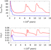 |
Fig. C.1. Evolution of the amplitude of libration of the resonant angle ζmax − ζmin (top) and mean eccentricities (bottom) for co-orbitals (m1/m2 = 6) captured in a 4:3 MMR with an outer planet such that m3/m1 = 1 (blue), m3/m1 = 1.6 (purple) and m3/m1 = 2.5 (red). The solid lines show the eccentricity of m2, while the dashed ones show the eccentricity of m1. Both amplitudes of libration and mean eccentricities are taken over a single libration period. These trajectories correspond to 3 cases of the top-right panels of Figs. C.2 and C.3. |
The effect of the relative masses between the co-orbitals m1 and m2, and the 3rd planet m3 is studied by integrating a grid of initial conditions, taking for the co-orbitals a1 = a2 = 1 au, ζ = 20° (which yield an amplidue of libration of 320°, hence a horseshoe configuration), and masses m1/m2 in the [1:20] range. Both the 3:2 and 4:3 MMR are studied. The mass of the 3rd planet is m3 = 3 × 10⁻⁵m0 when it is at a larger semi-major axis than the co-orbitals, and m3 = 1 × 10⁻⁵m0 when it is at a smaller semi-major axis. All eccentricities and inclinations are initially set to 0. τaj = 10/mj, and τej = τaj/150, which are consistent with the parameters of the disc described in Sect. 4.2 and Tanaka & Ward (2004). We set K = 0 (τaj independent from aj). Each initial condition (each set of masses) is integrated for 1.6 × 10⁵ years, which corresponds to a migration down to ≈0.4 au for the co-orbitals, depending on the chosen masses.
Results are displayed in Figs. C.2 and C.3. In both figures white pixels represent the systems for which the co-orbitals were not in the intended resonance with m3 at the end of the simulation. For the systems close to m3 = m1, the planet did not converge or did not converge fast enough to reach the desired resonance during the simulation. For the other white pixels, the desired resonance was crossed but the capture did not happen, or did not hold.
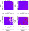 |
Fig. C.2. Effect of the capture into the 3:4 and 2:3 mean motion resonance for a pair of co-orbital planets m1 and m2 initially in a horseshoe configuration. The co-orbitals start with an amplitude of libration of ζmax − ζmin = 320°. The colour code represents the amplitude at the end of the simulation. In most cases, the capture in MMR with another planet tends to greatly reduce the amplitude of libration of the co-orbitals’ resonant angle. White pixels represent the systems for which the co-orbitals were not in the intended resonance with m3 at the end of the simulation. See the text for more details. |
In Fig. C.2, each pixel represents the final amplitude of libration of the co-orbital configuration for that set of masses. In almost all the studied cases, the capture into a mean-motion resonance with another planet led the co-orbital configuration to greatly reduce its own amplitude of libration, going from horseshoe to trojan configuration.
Figure C.3 shows the evolution of the amplitude of libration of the co-orbitals once they are captured in the MMR with m3. The set of integrations is the same as in Fig. C.2. The quantity −d(ζmax − ζmin)/da is obtained by comparing the amplitude of libration of the co-orbitals between t = [tmax/3 : 2tmax/3] and [2tmax/3 : tmax]. Areas of blue or purple pixels follow a similar behaviour to the blue example of Fig. C.1, where the amplitude of libration keeps decreasing post-capture. Orange or yellow pixels show mass ratios for which the amplitudes of libration are, on average, increasing post-capture. For comparison, in absence of m3 these co-orbital configurations would be diverging from the equilibrium for all values of m1/m2 = (1 : 20], since in these examples, K = 0 (see Fig. 7). The dependency of the stability with respect to the mass ratios is obviously complex and will be the object of a future study. We can nonetheless see from Figs. C.2 and C.3 that resonant chains can have a stabilising effect on the co-orbital configuration.
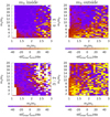 |
Fig. C.3. Evolution of the amplitude of the libration of the resonant angle ζmax − ζmin (with respect to the evolution of the semi-major axis) once the co-orbitals are captured in a mean-motion resonance with another planet. The systems are the same as in Fig. C.2. Purple colour indicates that the co-orbitals keep converging toward the exact resonance (L4 or L5), while yellow indicates that the amplitude is increasing post-capture. White pixels represent the systems for which the co-orbitals were not in the intended resonance with m3 at the end of the simulation. See the text for more details. |
Appendix D: Forces partial derivatives
The forces applied by the disc on each planet during the hydrodynamical simulations were saved with a time-step of 0.05 year. To compute the partial derivatives  and
and  we first performed a sliding averaging of the quantities Γj and Rj over the local orbital period, in order to get rid of short terms effect, notably the oscillations due to the eccentricities. The raw torque and the result of this averaging are displayed in black and red in Fig. D.1, respectively, in the case m1 = 6 M⊕ (leading), m2 = 12 M⊕ (trailing), discussed in Sect. 4.
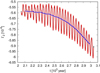 |
Fig. D.1. Torque applied on the 12 M⊕ planet in the 6 M⊕, 12 M⊕ case. |
Then we computed Γj0 and Rj0 by performing an additional sliding average over the local libration period. This period was computed by frequency analysis of the resonant angle ζ. For our example, the instantaneous value of Γ20 is displayed in blue in Fig. D.1. The quantity Γj − Γj0 is shown in Fig. D.2, with respect to the variable Δ and time (colour code). As we made a linear approximation in the neighbourhood of Δ = z = 0 in the analytical part of the study, we fitted ΓjIΔ + Γjζz to the quantity Γj − Γj0. Here again, this fit is done over a sliding window of width 1-libration period.
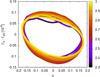 |
Fig. D.2. Γ2 vs. Δ in the 6 M⊕ 12 M⊕ case. The colour code is the time in [103 year]. |
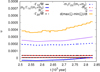 |
Fig. D.3. Temporal evolution of the terms of u in the 6 M⊕, 12 M⊕ case. |
Appendix E: Evolution of eccentricity under mass change
In the conservative case, described in Sect. 2.3.1, the diagonalisation is obtained by a change of variable X = PX𝒳, where the columns of the matrix PX are proportional to the eigenvectors of the matrix MX (this change is thus not unique). In the case of evolving masses, the matrix PX is not constant. We obtain the following relation:
We hence look for a change of variables 𝒳 = P𝒳X that diagonalises M𝒳 at second order in ε. To do so, we look for a change of basis ε close to PX:  . Noting P𝒳[j, k] the kth element of the jth line, the chosen change of basis is:
![$$ \begin{aligned}&P_{\mathcal{X} }[1,1] =m_2 \mathrm{e}^{i \frac{\pi }{3}} \nonumber \\&P_{\mathcal{X} }[1,2] = \mathrm{e}^{i \frac{\pi }{3}} + \frac{\varepsilon \mathrm{e}^{-i \frac{\pi }{6}}}{g_{L_4}} \left( \frac{\dot{X}_{1,d}}{X_1}- \frac{\dot{X}_{2,d}}{X_2} \right)\nonumber \\&P_{\mathcal{X} }[2,1] =-m_1 + \frac{ \varepsilon i }{g_{L_4}} \left[ \dot{m}_1 - \frac{m_1}{m_2} \dot{m}_2 + m_1 \left( \frac{\dot{X}_{1,d}}{X_1}- \frac{\dot{X}_{2,d}}{X_2} \right) \right]\nonumber \\&P_{\mathcal{X} }[2,2] = 1 \end{aligned} $$](/articles/aa/full_html/2019/11/aa34486-18/aa34486-18-eq169.gif)
while M𝒳 reads:
where
The temporal evolution of the variable 𝒳j is hence simply given by 𝒳j(t) = 𝒳j(0)e(gj + rxj)t. Orbits along the eccentric Lagrangian equilibria are defined by 𝒳1 = 0, while those along the anti-Lagrangian equilibria are defined by 𝒳2 = 0. For both of these configurations, the evolution of the eccentricities can be estimated from the quantity  :
:
where  , and
, and  .
.
All Tables
Value of the different terms of the stability criterion u for different hydro simulations with identical initial conditions except for the masses of the co-orbitals, given in the first two columns.
All Figures
|
Fig. 1. Phase space of Eq. (12). The black line represents the separatrix between tadpole orbits (3 examples in red) and horseshoe orbits (in blue). The phase space is symmetric with respect to ζ = 180°. |
| In the text | |
|
Fig. 2. Left: eccentric Lagrangian equilibrium: e1 = e2, ϖ1 − ϖ2 = ζ = ±60° and right: anti-Lagrangian equilibrium. At first order in the eccentricities: m1e1 = m2e2, ϖ1 − ϖ2 = ζ + 180°. |
| In the text | |
|
Fig. 3. Evolution of |
| In the text | |
|
Fig. 4. Evolution of the position of L4, L3, L5, and the separatrix emanating from L3, in the direction of ζ with respect to CΓ, for |
| In the text | |
|
Fig. 5. Evolution of a trajectory in the ( |
| In the text | |
|
Fig. 6. Attraction criterion for the L4 and L5 equilibria in the dissipative case, for different values of m2/m1. The equilibria are attractive if K is below the curve, and repulsive if K is above. The grey squares represent the attraction limit for a horseshoe orbit and were derived numerically, see the text for more details. |
| In the text | |
|
Fig. 7. Stability threshold for the L4/L5 equilibria when the torque induced by the protoplanetary disc is modelled using Eq. (49). The configuration diverge when K is above the line and converge when it is below. |
| In the text | |
|
Fig. 8. Gas surface densities (left panel), disc aspect ratios (middle panel) and K (right panel) at t = 0 Myr (blue lines), 1 Myr (red lines), 2 Myr (yellow lines) and 3 Myr (purple lines) for a typical protoplanetary disc model. |
| In the text | |
|
Fig. 9. Top panel: temporal evolution of semimajor axis for a pair of co-orbital planets. Bottom panel: surface density index α (blue line), aspect ratio index f (red line), and corresponding K (yellow line) at the planets’ location over time. |
| In the text | |
|
Fig. 10. ζmax − ζmin and K′ over time. When K′ is positive, resonance is diverging, and when K′ is negative, the resonance is converging. The dashed lines show there K′ changes sign, indicating the change from convergence to divergence or vice versa. |
| In the text | |
|
Fig. 11. Evolution of the relative change in mass against the relative change in angular momentum for four different planets over time. Black squares denote the starting point for the planets, whilst black crosses denote where the planets finish. Regions above the black line act to stabilise the co-orbital resonance, whilst below the line destabilises. |
| In the text | |
|
Fig. 12. Final amplitude of libration and semi-major axis of the co-orbitals formed in 880 synthetic systems around a 0.1 Solar mass star. 12% of the system had co-orbitals at the end of the run. Isolated co-orbital pairs are displayed in black, while those that are in resonance with another planet are displayed in red. Horseshoe configurations have an amplitude of libration above 180° degree. Other configurations are trojan. |
| In the text | |
|
Fig. 13. Panel a: comparing the torque from the disc between a − δr and a + δr (solid lines) on m1 = 5 M⊕ planet (red lines) and m2 = 3 M⊕ (blue lines). The lighter colours represent the torques from the simulations with a single planet and the darker ones for the co-orbital simulation. The same colour dotted lines mark the torque from the whole disc. The y-axis is the scaled torque and x-axis the distance from the planets’ orbit in unit of their mutual Hill radius RH. Panel b: perturbed surface density. Two horizontal lines are drawn at 1 and 5RH from the planets’ orbits to guide the eye. Panel c: torque on m2 as a function of distance from the planet. Panel a is the cumulative torque but this panel and panel d show the torque only from the grid cells at a given distance from the planet. The dashed and solid lines belongs to the outer and inner disc, respectively. The colour code is the same as in panel a. To ease the comparison, we plot the negative of the torque from the outer disc. The symbols mark where the torque on the planets change due to the presence of the second planet. Panel d: same as panel c but for m1. |
| In the text | |
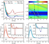 |
Fig. 14. Same as Fig. 13 but for m1 = 6 M⊕ and m2 = 12 M⊕. |
| In the text | |
|
Fig. 15. Upper panel: perturbed surface density for the models with a Jupiter and an Earth. The location of the low-mass planets are marked with + and × signs. Because the surface density perturbation is identical in both cases, we only show the surface density map of one of them but marked the location of both planets for comparison. The red, yellow, magenta, and grey lines mark different distances from the planets’ orbit. The dashed lines belong to the model with the low-mass planet at × and the solid lines are for the one with planet at +. These lines are also added to the lower panel to denote the effect of the Jupiter’s spirals. Lower panel: same as panel a of Fig. 13. The green and blue curves show the torque on the low-mass planet initiated close to L4 and L5 equilibria, respectively. The scaling is the Jupiter’s Hill radius RH for the x-axis and Γ0 for the y-axis that is calculated using the Jupiter’s mass. |
| In the text | |
|
Fig. 16. Evolution of torque (left) and radial force (right) on the Earth-mass planet in the leading case “×”. The black lines show the linear approximation for the evolution of these quantities with respect to Δ and ζ − ζeq, respectively. |
| In the text | |
|
Fig. 17. Evolution of the libration angle for models with m1 = 10 M⊕, m2 = 1 MJup and in discs with different values for αν and aspect ratio h. |
| In the text | |
|
Fig. 18. Example of attraction criteria in the eccentric directions in the dissipative case, for different values of m2/m1. For this example, the relations m1 = 10−4m0, τe1 = τe2m2/m1, and τa1 = 10/m1 were chosen. Orbits in the neighbourhood of L4 will tend toward e1 = e2 = 0 if τe2/τa1 is chosen below both curves of a given colour. The solid lines represent the stability limit in the anti-Lagrangian direction, while the dashed one is the limit in the eccentric Lagrangian direction, see the text for more details. |
| In the text | |
|
Fig. 19. Examples of the evolution of the quantities e2 and Δϖ for different initial conditions. The black dashed lines represent the direction of the anti-Lagrangian configuration while the black solid line is the direction of the Eccentric Lagragian equilibria. In both cases, the initial conditions are ω2 = ω1 + π, I1 = I2 = 0, m1 = 10m2 = 1 × 10⁻⁴m0, a1 = a2 = 1 au, e1 = 0.1, e2 = m1e1/m2 and ζ = 60°. Each trajectory is integrated for 20 Kyr, with the initial conditions represented by the black triangle, and the colour code representing the time (blue at t = 0, yellow at 20 Kyr). On the left panel, τe2/τa1 = 5, while on the rightτe2/τa1 = 20. In both cases, τa1/τa2 = 0.01. |
| In the text | |
|
Fig. 20. Examples for the evolution of I2 and Ω1 − Ω2. In both cases, the initial conditions are Ω2 = Ω1 + π + 0.3, I2 = 2°, m1 = 10m2 = 1 × 10⁻⁴m0, a1 = a2 = 1 au, e1 = e2 = 0 and ζ = 60°. Each trajectory is integrated for 20 Kyr, with the initial conditions represented by the black triangle, and the colour code representing the time (blue at t = 0). In the left panel, τI2/τa1 = 1, while on the rightτI2/τa1 = 30. In both cases, τa1/τa2 = 0.01. |
| In the text | |
|
Fig. C.1. Evolution of the amplitude of libration of the resonant angle ζmax − ζmin (top) and mean eccentricities (bottom) for co-orbitals (m1/m2 = 6) captured in a 4:3 MMR with an outer planet such that m3/m1 = 1 (blue), m3/m1 = 1.6 (purple) and m3/m1 = 2.5 (red). The solid lines show the eccentricity of m2, while the dashed ones show the eccentricity of m1. Both amplitudes of libration and mean eccentricities are taken over a single libration period. These trajectories correspond to 3 cases of the top-right panels of Figs. C.2 and C.3. |
| In the text | |
|
Fig. C.2. Effect of the capture into the 3:4 and 2:3 mean motion resonance for a pair of co-orbital planets m1 and m2 initially in a horseshoe configuration. The co-orbitals start with an amplitude of libration of ζmax − ζmin = 320°. The colour code represents the amplitude at the end of the simulation. In most cases, the capture in MMR with another planet tends to greatly reduce the amplitude of libration of the co-orbitals’ resonant angle. White pixels represent the systems for which the co-orbitals were not in the intended resonance with m3 at the end of the simulation. See the text for more details. |
| In the text | |
|
Fig. C.3. Evolution of the amplitude of the libration of the resonant angle ζmax − ζmin (with respect to the evolution of the semi-major axis) once the co-orbitals are captured in a mean-motion resonance with another planet. The systems are the same as in Fig. C.2. Purple colour indicates that the co-orbitals keep converging toward the exact resonance (L4 or L5), while yellow indicates that the amplitude is increasing post-capture. White pixels represent the systems for which the co-orbitals were not in the intended resonance with m3 at the end of the simulation. See the text for more details. |
| In the text | |
|
Fig. D.1. Torque applied on the 12 M⊕ planet in the 6 M⊕, 12 M⊕ case. |
| In the text | |
|
Fig. D.2. Γ2 vs. Δ in the 6 M⊕ 12 M⊕ case. The colour code is the time in [103 year]. |
| In the text | |
|
Fig. D.3. Temporal evolution of the terms of u in the 6 M⊕, 12 M⊕ case. |
| In the text | |
Current usage metrics show cumulative count of Article Views (full-text article views including HTML views, PDF and ePub downloads, according to the available data) and Abstracts Views on Vision4Press platform.
Data correspond to usage on the plateform after 2015. The current usage metrics is available 48-96 hours after online publication and is updated daily on week days.
Initial download of the metrics may take a while.