| Issue |
A&A
Volume 630, October 2019
|
|
|---|---|---|
| Article Number | A118 | |
| Number of page(s) | 16 | |
| Section | Extragalactic astronomy | |
| DOI | https://doi.org/10.1051/0004-6361/201936217 | |
| Published online | 02 October 2019 | |
The X-ray properties of z > 6 quasars: no evident evolution of accretion physics in the first Gyr of the Universe
1
Instituto de Astrofisica and Centro de Astroingenieria, Facultad de Fisica, Pontificia Universidad Catolica de Chile, Casilla 306, Santiago 22, Chile
e-mail: This email address is being protected from spambots. You need JavaScript enabled to view it.
2
Chinese Academy of Sciences South America Center for Astronomy, National Astronomical Observatories, CAS, Beijing 100012, PR China
3
Department of Astronomy & Astrophysics, 525 Davey Lab, The Pennsylvania State University, University Park, PA 16802, USA
4
Institute for Gravitation and the Cosmos, The Pennsylvania State University, University Park, PA 16802, USA
5
Department of Physics, The Pennsylvania State University, University Park, PA 16802, USA
6
Millennium Institute of Astrophysics (MAS), Nuncio Monseñor Sótero Sanz 100, Providencia, Santiago, Chile
7
Space Science Institute, 4750 Walnut Street, Suite 205, Boulder, CO 80301, USA
8
INAF – Osservatorio di Astrofisica e Scienza dello Spazio di Bologna, Via Gobetti 93/3, 40129 Bologna, Italy
9
School of Astronomy and Space Science, Nanjing University, Nanjing 210093, PR China
10
Key Laboratory of Modern Astronomy and Astrophysics (Nanjing University), Ministry of Education, Nanjing, Jiangsu 210093, PR China
11
Department of Physics, University of North Texas, Denton, TX 76203, USA
12
Dipartimento di Fisica e Astronomia, Università degli Studi di Bologna, via Gobetti 93/2, 40129 Bologna, Italy
13
15 Center for Astrophysics | Harvard & Smithsonian, 60 Garden St, Cambridge, MA 02138, USA
Received:
1
July
2019
Accepted:
26
August
2019
Abstract
Context. X-ray emission from quasars (QSOs) has been used to assess supermassive black hole accretion properties up to z ≈ 6. However, at z > 6 only ≈15 QSOs are covered by sensitive X-ray observations, preventing a statistically significant investigation of the X-ray properties of the QSO population in the first Gyr of the Universe.
Aims. We present new Chandra observations of a sample of 10 z > 6 QSOs, selected to have virial black-hole mass estimates from Mg II line spectroscopy  . Adding archival X-ray data for an additional 15 z > 6 QSOs, we investigate the X-ray properties of the QSO population in the first Gyr of the Universe. In particular, we focus on the LUV − LX relation, which is traced by the αox parameter, and the shape of their X-ray spectra.
Methods. We performed photometric analyses to derive estimates of the X-ray luminosities of our z > 6 QSOs, and thus their αox values and bolometric corrections (Kbol = Lbol/LX). We compared the resulting αox and Kbol distributions with the results found for QSO samples at lower redshift, and ran several statistical tests to check for a possible evolution of the LUV − LX relation. Finally, we performed a basic X-ray spectral analysis of the brightest z > 6 QSOs to derive their individual photon indices, and joint spectral analysis of the whole sample to estimate the average photon index.
Results. We detect seven of the new Chandra targets in at least one standard energy band, while two more are detected discarding energies E > 5 keV, where background dominates. We confirm a lack of significant evolution of αox with redshift, which extends the results from previous works up to z > 6 with a statistically significant QSO sample. Furthermore, we confirm the trend of an increasing bolometric correction with increasing luminosity found for QSOs at lower redshifts. The average power-law photon index of our sample (⟨Γ⟩ = 2.20−0.34+0.39 and ⟨Γ⟩ = 2.13−0.13+0.13 for sources with < 30 and > 30 net counts, respectively) is slightly steeper than, but still consistent with, typical QSOs at z = 1 − 6.
Conclusions. All of these results indicate a lack of substantial evolution of the inner accretion-disk and hot-corona structure in QSOs from low redshift to z > 6. Our data hint at generally high Eddington ratios at z > 6.
Key words: methods: data analysis / galaxies: active / galaxies: nuclei / X-rays: galaxies / galaxies: high-redshift / quasars: general
© ESO 2019
1. Introduction
X-ray emission from accreting supermassive black holes (SMBHs), shining as quasars (QSOs), is thought to originate from inverse Compton scattering in the so-called “hot corona” of the UV/optical photons produced by the accretion disk via thermal emission (e.g., Galeev et al. 1979; Haardt & Maraschi 1991; Beloborodov 2017). The relative importance of the hot corona and the accretion disk to the total radiative output is usually parametrized with αox = 0.38 × log(L2 keV/L2500 Å), which represents the slope of a nominal power-law connecting the rest-frame UV and X-ray emission (e.g., Brandt & Alexander 2015, and references therein). It is important to note that αox is known to anti-correlate with the QSO UV luminosity (e.g., Steffen et al. 2006; Just et al. 2007; Lusso & Risaliti 2016, see Lusso & Risaliti 2017, for a physical interpretation), that is, the fractional disk contribution to the total emitted power increases for more luminous QSOs. Most previous works (e.g., Vignali et al. 2003; Steffen et al. 2006; Just et al. 2007; Jin et al. 2012; Marchese et al. 2012; Lusso & Risaliti 2016; Nanni et al. 2017) found no evidence for evolution with redshift of αox. Recently, Risaliti & Lusso (2019) exploit this apparent lack of evolution to propose QSOs as standard candles to infer cosmological parameters (see also Salvestrini et al. 2019).
Currently, ≈200 QSOs have been discovered at z ≥ 6, corresponding to about the first Gyr of the Universe (Bañados et al. 2016, and references therein; Mazzucchelli et al. 2017; Reed et al. 2017, 2019; Tang et al. 2017; Wang et al. 2017, 2018a,b; Chehade et al. 2018; Matsuoka et al. 2018a,b, 2019; Yang et al. 2019; Fan et al. 2019; Pons et al. 2019), with ULAS J1342+0928 holding the redshift record of z = 7.54 (Bañados et al. 2018a). These rare QSOs were selected in wide-field optical/near-IR surveys such as SDSS, CFHQS, UKIDSS, Pan-STARRS1, ATLAS, and VIKING, and represent the extreme tail of the underlying SMBH population at early epochs. For instance, most of the known z > 6 QSOs are extremely luminous (log Lbol/L⊙ ≈ 12 − 14) and massive (up to ≈1010 M⊙; Wu et al. 2015). The very existence of such massive black holes (BHs) in the early universe challenges our theoretical knowledge of SMBH formation and early growth (e.g., Woods et al. 2019, and references therein). In particular, in order to match the observed masses at z ≈ 6 − 7, BH-seed models require extended periods of (possibly obscured) Eddington-limited1, or even super-Eddington accretion, during which the structure and physics of the accretion may be different than at lower redshift, where QSOs are typically characterized by somewhat lower Eddington ratios (e.g., Shen & Kelly 2012). This could produce a change in the αox − LUV relation at high redshift.
Several works have compared the optical/UV continuum and emission-line properties (e.g., De Rosa et al. 2014; Shen et al. 2019) of QSOs at z > 6 and at lower redshifts, generally finding a lack of evident evolution. However, the fraction of weak-line QSOs (WLQs, i.e., objects with C IV and Lyα+N V rest-frame equivalent widths REW < 10 Å and REW < 15 Å, respectively; for instance Fan et al. 1999; Diamond-Stanic et al. 2009) has been suggested to increase toward high redshift (e.g., Luo et al. 2015; Bañados et al. 2016), in spite of the color selection used for z > 6 QSOs that may be biased against objects with weak Lyα lines (Bañados et al. 2016). Since WLQs accrete preferentially with high Eddington ratios (e.g., Luo et al. 2015; Marlar et al. 2018), the higher fraction of WLQs may indicate that the known QSOs at z > 6 generally accrete at higher Eddington ratios than at lower redshift, which is consistent with previous findings (e.g., Wu et al. 2015). Shen et al. (2019) find an excess of WLQs at z > 5.7 compared to lower redshifts. Meyer et al. (2019) report a strong increase in the typical blueshift of the C IV emission line in QSOs at z ≳ 6, which can be linked again with the presence of a higher fraction of WLQs at high redshift (e.g., Luo et al. 2015). About half of the WLQ population is found to emit significantly weaker X-ray radiation than what is expected based on the UV luminosity (e.g., Ni et al. 2018). This is possibly linked to shielding by a geometrically thick inner accretion disk (e.g., Luo et al. 2015) as expected in the case of high Eddington-rate accretion.
X-ray observations can provide useful insights into the accretion physics in an independent way and on smaller scales than those probed by optical/UV emission. For instance, in addition to the αox parameter (e.g., Lusso & Risaliti 2017), the intrinsic photon index (Γ) of the hard X-ray power-law continuum carries information about the coupling between disk emission and the corona, and it is considered a proxy of the accretion rate. The relation between Γ and the Eddington ratio has been established over a range of redshifts for sizable samples of sources: steeper slopes correspond to higher implied Eddington ratios (e.g., Shemmer et al. 2008; Risaliti et al. 2009; Brightman et al. 2013; Fanali et al. 2013, but see also Trakhtenbrot et al. 2017a).
Despite the large number of z > 6 QSOs discovered to date, only ≈15 (i.e., ≈8% of the known population at these redshifts) are currently covered by sensitive pointed or serendipitous X-ray observations and only 11 are detected. This drastically limits our ability to use X-rays to investigate the accretion physics and structure in QSOs in the early universe. In this work, we present new Chandra observations for a sample of 10 QSOs at z > 6. Along with archival data, we use these observations to constrain the X-ray properties of QSOs at z > 6, derive the αox and Γ parameters, and study possible dependencies upon redshift and luminosity. Our targets were selected to have virial estimates for BH masses from the Mg II emission line, allowing us to include Eddington ratios in our analysis. We adopt a flat cosmology with H0 = 67.7 km s−1 and Ωm = 0.307 (Planck Collaboration XIII 2016).
2. The sample of z > 6 QSOs
2.1. Targets of new X-ray observations
We obtained Chandra observations of a sample of ten type 1 QSOs at z = 6.0 − 6.8 (Tables 1 and 2), with virial estimates of MBH from near-IR spectroscopy (using the Mg II line2; e.g., Vestergaard & Osmer 2009). The targets were selected to be radio-quiet or, at most, radio-moderate QSOs (see Sect. 2.3). Five of them have absolute magnitudes −26.2 < M1450 Å < −25.6 (see red symbols in Fig. 1), close to the break luminosity regime of the QSO luminosity function at z ≈ 6 (corresponding to M1450 Å ≈ −24.9; Matsuoka et al. 2018c). This allows us to push the investigation of the X-ray emission of high-redshift QSOs down to a luminosity regime between typical SDSS QSOs (e.g., Pâris et al. 2018) and the fainter QSOs discovered by the SHELLQ survey (Matsuoka et al. 2016). This region of the QSO L − z parameter space has been probed poorly to date at X-ray wavelengths. In fact, the only four M1450 Å > −26 QSOs at z > 6 with previous X-ray data were serendipitously covered by X-ray observations (i.e., they were not targeted) and are not detected. Notably, with our new observations we more than triple the number of QSOs observed in X-rays at the highest redshifts (z > 6.5). The distributions of the absolute and apparent magnitudes at rest-frame 1450 Å (M1450 Å and m1450 Å, respectively) as a function of redshift are shown in Fig. 1 (top and middle panels), and are compared with known z > 6 QSOs not observed in the X-rays.
Physical properties of z > 6 QSOs with new or archival X-ray observations.
Summary of our new Chandra and archival X-ray observations of z > 6 QSOs.
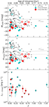 |
Fig. 1. Top and middle panels: distribution of M1450 Å and m1450 Å as function of redshift. Small black open circles are QSOs not covered by X-ray observations (Bañados et al. 2016; Mazzucchelli et al. 2017; Reed et al. 2017; Tang et al. 2017; Wang et al. 2017, 2018a,b; Chehade et al. 2018; Matsuoka et al. 2018b,a; Yang et al. 2019). Cyan symbols are QSOs with archival X-ray data (see Table 1). Red symbols are QSOs covered by the new X-ray observations presented in this work. Filled symbols are X-ray detected, open symbols are not detected. Dashed lines represent the break magnitudes of the QSO luminosity function (Matsuoka et al. 2018c). The dotted line represents our magnitude selection. Bottom panel: X-ray luminosity (derived as described in Sect. 3) as a function of redshift. Symbols are the same as above, but upper limits on X-ray luminosity for undetected QSOs are shown as downward-pointing triangles. |
2.2. Other z > 6 QSOs observed in X-rays
Nanni et al. (2017) studied the X-ray properties of all of the QSOs at z > 5.7 previously covered by pointed or serendipitous X-ray observations, 14 of which are at z > 6. We include in our analysis these 14 z > 6 QSOs. For these sources we used the magnitudes at 1450 Å provided by Bañados et al. (2016). We also include ULAS J1342+0928, which was discovered after the Nanni et al. (2017) work, and whose X-ray properties, magnitudes, and black-hole mass have been presented by Bañados et al. (2018a,b). We thus include in our analysis a total of 15 z > 6 QSOs with sensitive3 archival observations in the X-ray band.
Seven of these QSOs were observed by Chandra only, three by XMM-Newton only, four by both Chandra and XMM-Newton, and one by Swift. Recently SDSS J1030+0524 has been the target of a long Chandra imaging campaign (≈480 ks, Nanni et al. 2018), and was previously observed with both Chandra (with a shallow 8 ks observation; Brandt et al. 2002) and XMM-Newton (75 ks after background filtering; Farrah et al. 2004). However, considering the long separation between the old and new observations (≈10 − 15 years in the observed frame), and the hints for strong variation affecting its flux during this timespan, as discussed in Nanni et al. (2018), we limited our analysis to the deep 2017 Chandra dataset. Similarly, we consider only the ≈80 ks Chandra observation of SDSS J1148+5251 (Gallerani et al. 2017), and discarded a 2004 XMM-Newton observation with a nominal exposure time of ≈26 ks, which is however almost completely affected by background flaring. As a result, for nine QSOs out of the 15 objects with archival observations we used only Chandra data, for 3 QSOs we used only XMM-Newton data, for 2 QSOs we used data from both observatories, and for one we used Swift data (see Table 2).
We searched the literature to retrieve black-hole mass estimates for these 15 QSOs (see Table 1). Since different authors used different calibrations to obtain estimates of black-hole masses, we recalibrate the values found in the literature to match the calibration of Vestergaard & Osmer (2009), as marked in Table 1. We also modified luminosities and masses for our chosen cosmology. Furthermore, for consistency, we applied the same X-ray analysis (see Sect. 3) to these archival observations.
2.3. General properties of the sample
The main physical properties of our sample are reported in Table 1. For many of our targets, slightly different redshift values are reported in the literature, derived from the Mg II (2799 Å) and [C II] (158 μm) emission lines. When a [C II] measurement is available, we adopt it since the [C II] line is considered a better indicator of the systemic redshift than the Mg II line (e.g., Decarli et al. 2018), which sometimes displays significant blueshifts in the observed wavelength (e.g., Plotkin et al. 2015; Shen et al. 2016), possibly due to outflowing material in the broad emission-line region (e.g., ≈1700 km s−1 for SDSS J0109−3047, corresponding to Δz ≈ 0.04; Venemans et al. 2016).
We computed the bolometric luminosities (Lbol) consistently for all our targets using the bolometric correction of Venemans et al. (2016), which was also used in Decarli et al. (2018):  . The typical uncertainty on Lbol derived with this relation is ∼7%. We thus provide homogeneously derived Lbol rather than compiling values found in the literature, which are derived using different indicators of the bolometric luminosity (i.e., L3000 Å and M1450 Å) and different bolometric corrections.
None of the QSOs included in our sample has been detected in the FIRST (which covers 16 of the 25 QSOs in our sample; Becker et al. 1995) or NVSS (covering all of our z > 6 QSOs; Condon et al. 1998) radio surveys. We report in Table 1 the radio-loudness parameter R = fν,5 GHz/fν,4400 Å (Kellermann et al. 1989), i.e., the ratio of the flux densities at rest-frame 5 GHz and 4400 Å, or its upper limit, for the QSOs in our sample. R values of QSOs included in the compilation of Bañados et al. (2015b) are taken from that work, including the only two QSOs detected at 1.4 GHz (with R = 0.7 − 0.8). For the remaining sources, we derived fν,4400 Å from m1450 Å (Col. 5 of Table 1), assuming a power-law continuum with α = −0.3, following Bañados et al. (2016). Upper limits on the radio emission at 1.4 GHz are derived as 3 × rms of the FIRST or NVSS surveys. For CFHQS J0216−0455, we used the rms of the VLA observations in the SXDS field (Simpson et al. 2006). Finally, we estimated the upper limits on fν, 5 GHz assuming a power-law spectrum with α = −0.75. Based on their upper limits on R, all of our sources are either radio-quiet (R < 10) or at most radio-intermediate (R < 40). We thus do not expect their X-ray emission to be significantly affected by a jet-linked contribution (e.g., Miller et al. 2011). Bañados et al. (2015b) reported a radio-loud QSO fraction of ≈8% among the z ≈ 6 population. The only three radio-loud QSOs at z > 6 are not covered by X-ray observations and thus are not included in our sample.
It is difficult to establish firmly how many of the QSOs in the sample can be classified as WLQs, mainly because of the limited quality of the optical/UV spectra and spectral coverage. Beside the known WLQ SDSS J0100+2802 (Wu et al. 2015), other WLQ candidates are VIK J0109−3047, ULAS J1342+0928, and SDSS J2310+1855, all with REW(C IV)≈10 − 15 (see Table 1 for the spectral references). However, several of the sources lack measurements of REW(C IV). Furthermore, as reported in Table 1, two QSOs are classified as broad absorption-line QSOs (BALQSOs), which usually show weak X-ray emission as well (e.g., Gallagher et al. 2006; Gibson et al. 2009; Wu et al. 2010; Luo et al. 2014).
3. Data analysis
3.1. X-ray data reduction
Table 2 summarizes the basic information about the X-ray observations of our new targets and archival sources. We reprocessed the Chandra observations with the chandra_repro script in CIAO 4.104, using CALDB v4.8.15, setting the option check_vf_pha=yes in the case of observations taken in very faint mode. We created exposure maps with the fluximage script. Spectra, response matrices, and ancillary files for sources and associated background were extracted using the specextract tool.
SDSS J1030+0524 has been observed with ACIS-I in ten individual pointings over five months, for a total of ≈480 ks (see Table 2 and Nanni et al. 2018). Similarly, VIK J0109–3047, SDSS J1306+0356, ULAS J1342+0928, and CFHQS J1641+3755 have been targeted with two Chandra observations, for a total of ≈65, 126, 45, and 54 ks, respectively (see Table 2 and Bañados et al. 2018b). For these sources, we checked for astrometry issues and merged the individual observations with the reproject_obs tool, and derived merged images and exposure maps. In doing this, we effectively combine the different pointings into a single, longer exposure. Spectra, response matrices, and ancillary files extracted from the single pointings were added using the mathpha, addrmf, and addarf HEASOFT tools6, respectively, weighting by the individual exposure times.
XMM-Newton observations have been processed with SAS v16.1.0., following the standard procedure7 and filtering for periods of high background levels imposing count-rate thresholds of < 0.4 and < 0.35 cts s−1 in the 10 < E < 12 keV and E > 10 keV bands for the EPIC/PN and EPIC/MOS cameras, respectively. We created images and exposure maps, and extracted spectra, response matrices, and ancillary files using the evselect, eexpmap, backscale, rmfgen, and arfgen tools.
In the case of sources targeted by multiple XMM-Newton pointings (i.e., CFHQS J0210−0456 and ULAS J1120+0641; see Table 2), we merged the different datasets for each EPIC camera with the merge tool, and, similarly to what we did for Chandra sources, we added the spectra extracted from each observation with the epicspeccombine tool. We also averaged the response matrices and ancillary files with the addrmf and addarf tools, weighting by the exposure times of the individual observations. We note that epicspeccombine returns as output a summed spectrum with exposure time set to the average value of the two input spectra, and the sum of the two input ancillary files. This is the equivalent of observing the source for half of the total time with a fictional camera with twice the sensitivity of the actual camera. By changing with dmhedit the exposure time keyword of the output summed spectrum to the summed exposure time of the two input spectra, and by computing the weighted average of the response matrices and ancillary files with addrmf and addarf, we return to the case in which the source is observed by the actual camera for a longer exposure time. The two cases are equivalent when spectra and ancillary files are used together (e.g., performing spectral analysis with XSPEC). However, in Sect. 3.3 we will use the ancillary files alone to compute the count-rate to flux conversion factors. In such a case, the use of the summed ancillary files obtained as output of epicspeccombine would not be correct.
We then used the merged images to compute source photometry (see Sect. 3.2). Since these sources were placed at similar off-axis angles in the different pointings, by merging the observations for each camera we effectively combine them into single and longer observations. However, we keep the different cameras separated, as the responses are significantly different. We then combined the scientific results, as described in Sect. 3.3.
We reduced Swift-XRT data for ATLAS J0142−3327 as in Nanni et al. (2017), using the standard software (HEADAS v. 6.18)8 and procedures9. An ancillary file has been extracted with the xrtmkarf tool.
3.2. Detection procedure
For Chandra observations, we used circular source extraction regions centered on the optical positions of the targets and with radii of 2 arcsec, to account for X-ray and optical positional uncertainties, and any possible small X-ray-to-optical offset. This region size encompasses ≈100% and ≈90% of the Chandra PSF at E = 1.5 and 6.4 keV, respectively, for an on-axis position. The background levels are evaluated in local annular regions centered on the targets, with inner and outer radii of 4 and 24 arcsec, respectively, free of contaminating sources. All the sources in our sample covered by Chandra observations were observed on axis, except for SDSS J0303−0019, which is observed at an off-axis angle of ≈4.8 arcmin.
For XMM-Newton observations, we used circular source extraction regions centered on the optical positions of the targets and with radii of 10–30 arcsec (corresponding to ≈50 − 80% of the PSF), depending on the off-axis angle of the source (0 − 6 arcmin) and the presence of nearby detected objects that could contaminate the photometry. Circular background extraction regions are placed at nearby locations free of evident detected sources and have radii of 60–80 arcsec. For the Swift-XRT observation of ATLAS J0142−3327 we computed the source photometry in a circular region with radius 10 arcsec, which equates to ≈50% of the PSF (Moretti et al. 2005), and the background photometry in a nearby circular region with radius ≈72 arcsec.
We ran the detection procedure in three energy bands (0.5 − 2, 2 − 7, and 0.5 − 7 keV, which we refer to as the soft, hard, and full bands, respectively) separately for every available instrument (ACIS, EPIC/PN, EPIC/MOS1, EPIC/MOS2, and XRT). Different images of one object taken with the same instrument were merged, as described in Sect. 3.1. We computed the detection significance in each energy band using the binomial no-source probability (Weisskopf et al. 2007; Broos et al. 2007)
 (1)
(1)
where S is the total number of counts in the source region in the considered energy band, B is the total number of counts in the background region, N = S + B, and p = 1/(1 + BACKSCAL), with BACKSCAL being the ratio of the background and source region areas. For sources observed by multiple instruments, we consider the quantity  as the final binomial no-source probability in one energy band, where the product is performed over all the instruments used to observe a source. We consider a source to be detected if (1 − PB) > 0.99. Out of the 111 analyzed images (25 objects in the three energy bands, some of which were observed by different instruments, see Table 3), we expect 111 × PB ≈ 1 false detection with the adopted significance threshold.
Observed X-ray photometry and hardness ratios.
Figure 2 displays the X-ray images of our new targets in the three energy bands (see Nanni et al. 2017 and Bañados et al. 2018b, for similar images for the archival sources). Detected and undetected sources are identified with green and red circles, respectively. Three of our 10 observed targets are detected in all of the three considered bands, four QSOs are detected in the soft and full bands only, and three are not detected in any band. Reasonably different sizes for the source and background extraction regions do not affect these results.
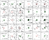 |
Fig. 2. Smoothed Chandra images (40 × 40 pixels; i.e., ≈20″ × 20″) of our ten new targets (rows, as annotated) in soft (first column), hard (second column), and full (third column) band. Circles represent the source extraction regions (R = 2 arcsec) centered on the optical positions of the targets, and used to compute source photometry. Green and red circles are used for detected and undetected sources, respectively. |
3.3. Photometry, fluxes, and luminosities
We computed the net counts and associated uncertainties (or upper limits in the case of non-detections) by deriving the probability distribution function of net counts with the method of Weisskopf et al. (2007, see their Appendix A3), which correctly accounts for the Poisson nature of both source and background counts. For sources detected by an instrument in one energy band, we report in Table 3 the nominal value of the net counts, corresponding to the peak of the probability distribution, and the errors corresponding to the narrowest 68% confidence interval. For undetected sources we report the upper limit corresponding to the 90% confidence interval. These values are not corrected for the fraction of PSF excluded in the extraction regions.
We used the probability distribution functions of the net counts in the soft and hard bands to constrain the hardness ratio HR = (H − S)/(H + S), where S and H are the observed net counts in the soft and hard bands, respectively: we randomly picked a pair of values following such functions and computed HR. Repeating the procedure 10 000 times, we constructed the probability distribution function of HR, and computed the 68% confidence interval, or 90% upper limit in the case of sources undetected in the hard band (Table 3). We found no significantly different hardness-ratio values using the Bayesian Estimation of Hardness Ratios (BEHR) code (Park et al. 2006). The last column of Table 3 reports the effective photon indices corresponding to the HR values, computed assuming a power law model and Galactic absorption (Kalberla et al. 2005), and accounting for the effective area of each instrument at the time of each observation and at the position of each source on the detector.
The probability distribution functions of X-ray flux in the three energy bands have been derived from the net count-rate probability distribution function assuming a power-law spectrum with Γ = 2.0 (typical of luminous QSOs, e.g., Shemmer et al. 2006a; Nanni et al. 2017, see also Sect. 4.3), accounting for Galactic absorption (Kalberla et al. 2005) and using the response matrices and ancillary files extracted at the position of each target. All of the ancillary files are corrected for the fraction of the PSF not included in the extraction regions. Thus, fluxes and derived quantities are corrected for PSF effects. Table 4 reports the fluxes corresponding to the peak of the probability distribution functions, and the uncertainties corresponding to the narrowest interval containing 68% of the total probability for sources detected in an energy band. For undetected objects we report the upper limit corresponding to the 90% probability.
X-ray fluxes, luminosities, and derived properties for our Chandra and archival sample of z > 6 QSOs.
For QSOs observed by different instruments, we derived the flux probability distribution function for each instrument, multiplied them together and then renormalized the result to obtain the average distribution. This was used to compute the nominal fluxes and uncertainties. Deep observations produce narrower probability distribution functions than shallower pointings, and thus dominate the averaged final distribution. This averaging procedure works if a source did not vary strongly between the different observations; otherwise, the flux probability distribution functions for the individual instruments do not overlap and their product is null. There is no such case in our sample. We note, however, that for some objects observed by multiple instruments several months apart (e.g., SDSS J0100+2802 and ULAS J1120+0641), the flux probability distribution functions of the individual instruments are slightly shifted, although they still largely overlap. While this shift can be simply explained by statistical fluctuations of the measured counts, we cannot exclude some level of source variability. In this case our results would correspond to fluxes averaged over the different observed states. We note that Shemmer et al. (2017) report no significant evolution of QSO X-ray variability amplitude with redshift, at least up to z ≈ 4.3.
Luminosities in the rest-frame 2 − 10 keV band (Table 4) and monochromatic luminosities at 2 keV have been computed from the unabsorbed (i.e., corrected for Galactic absorption) fluxes in the soft band, assuming again Γ = 2.0. Figure 1 (bottom panel) presents the distribution of X-ray luminosity vs. redshift for z ≥ 6 QSOs. A short extrapolation is needed in the X-ray luminosity calculation, since the emission at rest-frame 2 keV is redshifted below 0.5 keV at z > 6, and is thus not directly probed by X-ray observations.
4. Results
4.1. αox vs. luminosity, redshift, and QSO properties
We computed L2500 Å from the 1450 Å magnitude assuming a power-law spectrum with α = −0.3, (e.g., Bañados et al. 2016; Selsing et al. 2016). Table 4 shows the αox values for the sources in our sample. The reported errors account only for the errors on the X-ray photometry, which dominate over the uncertainties on L2500 Å. Errors on the UV luminosities are dominated by the assumed UV spectral slope rather than measurement errors. For instance, assuming α = −0.5 (e.g., Vanden Berk et al. 2001) returns αox values steeper by ≈0.02 than the reported ones, and thus still well within the errors on αox reported in Table 4.
We plotted in Fig. 3 αox vs. UV luminosity for our sample, and compared them with the best-fit relations of Just et al. (2007), Lusso & Risaliti (2016), and Martocchia et al. (2017). All of these relations are very similar in the luminosity regime probed by our sources. We plot as small black symbols the sample of z < 6 QSOs (from Shemmer et al. 2006b; Steffen et al. 2006, and Just et al. 2007) used to fit the Just et al. (2007) relation. We also show the sample of > 2000 QSOs of Lusso & Risaliti (2016) as a color-coded map based on the number of sources per bin. For visual purposes only, we did not include upper limits (i.e., QSOs not detected in the X-rays) from Lusso & Risaliti (2016), which would populate preferentially the steep αox regime.
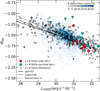 |
Fig. 3. αox vs. L2500 Å for z ≥ 6 QSOs. We compared our results with a compilation of optically selected QSOs at lower redshifts (Shemmer et al. 2006a; Steffen et al. 2006; Just et al. 2007; Lusso & Risaliti 2016). Downward pointing triangles represent upper limits. We also show the best-fitting relations of Just et al. (2007), Lusso & Risaliti (2016), and Martocchia et al. (2017). For visual purposes, we do not plot X-ray undetected sources included in the Lusso & Risaliti (2016) sample. |
In order to check if the αox values we found are in agreement with those expected from literature relations, we first note that the probability that a source is observed with an αox flatter or steeper than the expectation from a reference relation (we assumed the Just et al. 2007 one, based on optically selected QSOs as is our sample) due to random fluctuations only can be described by a binomial distribution, with probability of “success” p = 0.5 (i.e., we expect half of the sample to be above the relation), and number of trials n = 25 (i.e., the sample size). Assuming the two extreme cases in which upper limits on αox are treated as a detection (i.e., x = 13 sources above the relation) or represent sources intrinsically below the relation (i.e., x = 9), a binomial test returns probabilities of the observed or more extreme configurations given the expected configuration of P = 0.50 and P = 0.11, respectively. If we do not consider the four sources with weak upper limits on αox, which do not provide useful information, we find n = 21 and x = 9, corresponding to P = 0.33. According to these values, we do not find evidence supporting a significant variation of αox(L2500 Å) with redshift from this basic assessment.
This result can also be assessed by computing the difference between the observed αox and the value expected from the UV luminosity, according to the relation of Just et al. (2007), that is, Δαox = αox(observed) − αox(L2500 Å) as a function of redshift (Fig. 4). If αox(L2500 Å) does not vary significantly with redshift, we expect the Δαox distribution of our sample to be consistent with the distribution of the sample used by Just et al. (2007) to fit their relation. We test this null hypothesis (i.e., that the two Δαox distributions are drawn from the same population) using the univariate methods (Feigelson & Nelson 1985) included in ASURV Rev. 1.2 (Isobe & Feigelson 1990; Lavalley et al. 1992), which allows accounting for censored data (i.e., sources undetected in X-rays). The null-hypothesis probabilities for the several tests we ran are reported in Table 5. According to these tests, the Δαox distribution of our sample is consistent with those of lower-redshift samples collected from the literature. Finally, we computed the Kaplan–Meier estimator for the distribution function of the Δαox parameters of the considered samples. Results are summarized in Table 610. Following Steffen et al. (2006, see their Sect. 3.5), we can estimate roughly the allowed fractional variation of the typical UV-to-X-ray flux ratio in QSOs as δr/r = 2.606 ln(10)αox ≈ 6δαox = 0.16 at 1σ, where r = fν(2500 Å)/fν(2 keV) and δαox is the allowed variation of αox, which we approximated with the uncertainty on the mean of Δαox computed with the Kaplan–Meier estimator. This estimate may be somewhat optimistic, as, for instance, we did not take into account the uncertainties on the Just et al. (2007) αox − L2500 Å relation.
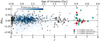 |
Fig. 4. Δαox vs. redshift for z ≥ 6 QSOs. We compared our results with a compilation of QSOs at lower redshifts (see Fig. 3). Downward-pointing triangles represent upper limits. The horizontal dashed line corresponds to Δαox = 0. |
Probabilities that Δαox distributions (including censored values) of our sample and samples taken from literature (Just et al. 2007 and Lusso & Risaliti 2016) are drawn from same parent population.
Results of Kaplan–Meier estimator for distribution function of Δαox for our z > 6 sample and lower-redshift samples from Just et al. (2007) and Lusso & Risaliti (2016).
In Fig. 5 we also compare the distribution of Δαox of our z > 6 QSOs with the sample of z ≈ 2 QSOs presented in Gibson et al. (2008, improved sample B; see Footnote 3 of Ni et al. 2018), which has been carefully selected to discard BALQSOs, and includes only X-ray detected QSOs. The two distributions are broadly consistent, again pointing toward a lack of a significant evolution of αox with redshift. We do not find a significant deviation of Δαox also limiting the tests to QSOs at the highest redshifts (z > 6.5) in our sample, although we note that the size of such a subsample is too small (7 QSOs, 3 of which undetected) to derive strong conclusions.
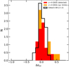 |
Fig. 5. Normalized histogram of Δαox for our sample of z > 6 QSOs (detections and upper limits are represented with red and orange histograms, respectively). We compared it with the sample of z ≈ 2 QSOs presented as sample B of Gibson et al. (2008). |
Based on the apparently non-evolving QSO LUV − LX relation across cosmic time, Risaliti & Lusso (2019) propose the use of QSOs up to z ≈ 5 as standard candles to infer cosmological parameters, finding evidence for a deviation from the concordance ΛCDM model. In this respect, since type Ia supernovae are detected up to z ≈ 1.4 only, QSOs are particularly useful in the distant universe.
We do not find evidence supporting a significant correlation between Δαox and MBH, bolometric luminosity, or λEdd: Spearman’s test returned ρ = −0.10 and P = 0.66, ρ = 0.04 and P = 0.84, and ρ = 0.24 and P = 0.29, respectively. We underline that Δαox factors out the dependence of αox with UV luminosity, which also enters into the computation of MBH and bolometric luminosity, and it is thus a better parameter to use when checking for any potential correlation with such quantities.
QSO emission variability is potentially a significant source of uncertainty affecting the derived values of αox and Δαox (e.g., Gibson & Brandt 2012; Vagnetti et al. 2013). For instance, Shemmer et al. (2005) detected X-ray flux variability of a factor of ≈4 for SDSS J02310–728 at z = 5.41 over a rest-frame period of ≈73 days. Nanni et al. (2018) found evidence for strong variability affecting the emission of SDSS J1030+0524 at z = 6.308 (see also Shemmer et al. 2005): its X-ray flux increased by a factor of ≈2.5 from an XMM-Newton observation in 2003 to the 2017 Chandra dataset analyzed in this work, corresponding to a variation of Δαox of ±0.16. As also discussed in Sect. 3.3, we do not find other similar cases among the few other QSOs covered by multiple observations.
4.2. Bolometric corrections
Figure 6 presents the X-ray luminosities of z > 6 QSOs plotted against their bolometric luminosities. We compare these with the sample of lower-luminosity Type 1 AGN selected in the XMM-COSMOS survey of Lusso et al. (2010), and with QSO samples with luminosities similar to or larger than those of our high-redshift sample (Feruglio et al. 2014; Banerji et al. 2015; Cano-Díaz et al. 2012; Martocchia et al. 2017; Ricci et al. 2017; Vito et al. 2018). In particular, our sample populates a luminosity regime in this plane poorly sampled before. The positions of our z > 6 sources confirm the trend of increasing bolometric correction Kbol = Lbol/LX with bolometric luminosity, from Kbol ≈ 10 − 100 at log Lbol ≲ 46.5 to Kbol ≈ 100 − 1000 at  , in agreement with previous works. We note that the bolometric luminosities of our type 1 QSOs are derived from the UV luminosities as described in Sect. 2.3, with typical relative uncertainties of ∼7%. Thus, the bolometric corrections found are byproducts of the relation shown in Fig. 3.
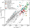 |
Fig. 6. X-ray vs. bolometric luminosity of our sample of z > 6 QOSs (red and cyan symbols). We compared our results with the compilation of lower luminosity QSOs of Lusso et al. (2012, empty gray circles). We also add the sample of luminous QSOs from Martocchia et al. (2017, green symbols), the Hot DOG samples of Vito et al. (2018, orange symbols; the orange star represents the stacked result of several Hot DOGs undetected in the X-rays) and Ricci et al. (2017, purple square), and results for some individual hyperluminous QSOs (filled gray symbols; see Martocchia et al. 2017 for their luminosities Feruglio et al. 2014; Banerji et al. 2015; Cano-Díaz et al. 2012). The dashed and dash-dotted black curves are the best-fitting relation of Lusso et al. (2012) and Duras et al. (in prep.), respectively. Downward pointing triangles represent upper limits. Diagonal dotted lines mark the loci of constant bolometric correction. |
4.3. Spectral analysis
4.3.1. Individual sources
We performed a basic spectral analysis for individual sources in our sample, considering only those detected in at least one energy band, in order to compare the resulting parameters with those derived from hardness-ratio and aperture photometry analyses (Tables 3 and 4). Spectra, response matrices, and ancillary files were extracted as described in Sect. 3.1. We fit the spectra with XSPEC v12.9.0n (Arnaud 1996)11. We used the W-statistic12, which extends the Cash (1979) statistic in the case of background-subtracted data. In the case of a source observed by more than one instrument, we performed a joint spectral analysis using all the available spectra. Due to the generally limited photon counting statistics, we assumed a simple power-law model, and included Galactic absorption along the line of sight of each source (Kalberla et al. 2005). The photon index and the power-law normalization are the only free parameters. Notwithstanding the simplicity of the model, the fit does not converge for SDSS J0842+1218 (which has ≈3 net counts), which is thus not considered hereafter. For two other sources, PSO J036+03, SDSS1048+5251, and SDSS J2310+1855, the fit converges but returns only an upper limit on the power-law normalization, and thus on flux and luminosity.
Best-fit parameters are reported in Table 7. Although the uncertainties are typically large, the results derived from spectral and hardness-ratio analyses are consistent, suggesting that the procedures used in the previous sections are robust. The luminosity derived for PSO J338+29 from spectral analysis is significantly larger than the value found from photometric analysis (Table 4), where we assumed Γ = 2.0. This is due to the extremely steep best-fitting photon index derived from spectral analysis, likely due to the limited photon-counting statistics.
4.3.2. Joint spectral analysis
We performed a joint spectral analysis to estimate the average photon index of sources detected in at least one energy band (18 sources). We removed the 6 QSOs with a total of more than 30 net counts in their spectra, for which results from individual spectral fitting are reported in Sect. 4.3.1, as they would dominate the spectral-fit results. We used a single power-law model with photon index free to vary, but linked among the datasets, to fit jointly the remaining 12 sources (≈115 net counts in the 0.5 − 7 keV band) and added Galactic absorption appropriate to each source. We found a best-fitting, average photon index  (errors at the 90% c.l. corresponding to ΔW = 2.7;
  with errors at the 68% c.l. corresponding to ΔW = 1.0)13. Repeating the joint spectral analysis for the 6 QSOs with > 30 net counts (≈746 net counts in total), we found an average
  (±0.08 at the 68% c.l.). Considering only QSOs at z > 6.5, ULAS1120+0641 is detected with > 30 counts, and its best-fitting photon index is Γ ≈ 2 (see Table 7). Joint spectral analysis of the other three z > 6.5 QSOs detected in the X-rays (≈23 net counts in total) returns
  (
( with errors at the 68% c.l.).
All of these values are slightly steeper than, although still consistent with, that found by Nanni et al. (2017) for z > 5.7 QSOs, thus including a subsample of our sources (i.e.,  ), and with the findings of Piconcelli et al. (2005), Vignali et al. (2005), Shemmer et al. (2006a), and Just et al. (2007) at lower redshifts (Fig. 7). Thus, we conclude there is no strong evidence supporting a significant systematic variation of Γ in our sample, although there are hints of a steepening of the typical QSO photon index at z > 6.
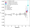 |
Fig. 7. Photon index as function of redshift. We report the individual best-fitting values for sources with > 30 total net counts (gray symbols), the results derived from joint spectral analysis of QSOs with > 30, < 30 net counts, and of z > 6.5 QSOs (red, blue, and cyan circles, respectively, plotted at the median redshift of each subsample), and the average photon indices derived by Piconcelli et al. (2005), Vignali et al. (2005), Shemmer et al. (2006b), Just et al. (2007), and Nanni et al. (2017) for optically selected luminous QSOs at different redshifts. Errors are at the 68% confidence level. |
The observed-frame 0.5 − 7 keV band corresponds to rest-frame energies at z > 6 where a possible Compton-reflection component would peak in the X-ray spectra of QSOs. We did not account for this component in the spectral fitting, due to the small number of total counts preventing the use of relatively complex models. However, we note that the reflection component in the X-ray spectra of luminous Type-1 QSOs has been found to be generally weak both in the local universe (e.g., Comastri et al. 1992; Piconcelli et al. 2005) and at high redshift (z > 4, e.g., Shemmer et al. 2005). Moreover, a strong reflection component would tend to flatten systematically the observed effective photon index, in contrast with our results.
Performing joint spectral analysis on subsamples of QSOs divided on the basis of their Eddington ratios, we do not find any significant trend of Γ with λEdd. However, this may be due to the small sample size, and the large uncertainties affecting the single-epoch black hole masses and the best-fitting photon indices.
In order to place a basic upper limit on the average column density, we added an XSPEC zwabs component and repeated the joint fit of QSOs with > 30 net counts. We left both the photon index and the column density free to vary, but linked them among the spectra, and fixed the redshift to the appropriate value for each QSO. The best-fitting parameters are  and NH < 9 × 1022 cm−2 at the 90% confidence level (see Fig. 8 for the confidence contours). The upper limit on NH is dominated by the high-redshift nature of the sources, which causes the photoelectric cutoff to shift below Chandra observed energy bands even for possible moderately high values of column density.
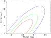 |
Fig. 8. Confidence contours at 68%, 90%, and 99% confidence levels (red, green, and blue curves, respectively) of best-fitting column density and photon index derived from joint spectral analysis of QSOs with > 30 counts (see Sect. 4.3.2). |
4.4. Comments on individual QSOs
4.4.1. PSO J167–13
This QSO (z = 6.515) falls slightly below our detection threshold in the hard band (PB = 0.989). We then checked whether we could detect it by restricting the detection energy range to the 2 − 5 keV band. This choice is motivated by the drop of the Chandra effective area and the relatively high background level at higher energies. Moreover, observed energies E > 5 keV correspond to E > 37.5 keV in the QSO rest frame, where the number of emitted X-ray photons is limited due to the QSO power-law spectrum.
An X-ray source is significantly detected (PB = 4 × 10⁻⁴) with  net counts in the 2 − 5 keV band in an R = 1 arcsec circular region (Fig. 9). The centroid of the X-ray emission shows an offset of ≈1 arcsec with respect to the optical position of the QSO, but with a positional uncertainty of 1.2 arcsec at the 90% confidence level. Considering the lack of counts detected in the soft band, following the procedure used in Sect. 3.3, we derived HR > 0.47 and HR > 0.08 at the 68% and 90% confidence levels, corresponding to Γeff < 0.55 and Γeff < 1.54, respectively. This very hard spectrum at z = 6.515, assuming an intrinsic Γ = 2 spectrum, corresponds to lower limits on the obscuring column density of NH > 2 × 1024 cm−2 and NH > 6 × 1023 cm−2 at the 68% and 90% confidence levels, respectively. Therefore this object is the first heavily obscured QSO candidate at z > 6, with the intriguing property of being an optically classified Type 1 QSO.
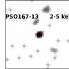 |
Fig. 9. Smoothed 2 − 5 keV image (40 × 40 pixels; ≈20″ × 20″) of PSO167–13. The red cross marks the optical position of the QSO. |
An ALMA sub-mm observation (Willott et al. 2017) revealed the presence of a close galaxy companion from the rest-frame UV and [C II] position of the QSO (0.9 arcsec; i.e., ≈5 kpc in projection at the redshift of the QSO), and by Δv ≈ −270 km s−1 (i.e., Δz ≈ 0.007) in velocity space. The offset between the X-ray centroid and the [C II] position of this galaxy is only ≈0.15 arcsec. A thorough investigation and discussion of this system has been presented separately (Vito et al. 2019).
4.4.2. VIK0305–3150
Similarly to PSO167–13, VIK0305–3150 (z = 6.047) is slightly below our detection threshold both in the hard and full bands. We thus repeated the analysis restricting the energy bands to 2 − 5 keV and 0.5 − 5 keV. We nominally detected this QSO in a R = 1 arcsec circular region in the 2 − 5 keV band with PB = 6.6 × 10⁻³, but with a very limited number of net counts ( ). The detection in the 0.5 − 5 keV band is more solid (PB = 1.1 × 10⁻³) with
  net counts (Fig. 10). Repeating the same hardness-ratio analysis as done above for PSO167–13, we found HR > 0.00 and HR > −0.39, corresponding to Γeff < 0.96 and Γeff < 1.93 at the 68% and 90% confidence levels, respectively. Assuming an intrinsic Γ = 1.9, the nominal obscuring column density is NH > 1 × 1024 cm−2 at the 68% confidence level, but it is not constrained at the 90% confidence level.
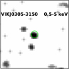 |
Fig. 10. Smoothed 0.5 − 5 keV image (40 × 40 pixels; ≈20″ × 20″) of VIK J0305–3150. The green circle has a radius R = 1 arcsec. |
4.4.3. CFHQS J1641+3755
This radio-quiet (R < 10.5) QSO at z = 6.047 has one of the lowest bolometric luminosities  and smallest black hole masses (
 ) among the z > 6 QSO sample, resulting in a high Eddington ratio (λEdd = 1.5). While the bolometric correction is usually found to anti-correlate with the Eddington ratio both observationally (e.g., Lusso et al. 2012) and theoretically (e.g., Meier 2012; Jiang et al. 2019, but see also Castelló-Mor et al. 2017), CFHQS J1641+3755 is the second most X-ray luminous z > 6 QSO, resulting in a bolometric correction Kbol ≈ 13. This is also reflected in a quite flat αox = −1.28. Considering an rms = 0.2 for the αox − LUV relation in the LUV luminosity range where CFHQS J1641+3755 lies (Steffen et al. 2006), this QSO is a ≈1.8σ outlier.
Its ≈50 net counts allowed us to constrain with a reasonable accuracy its photon index, which, as expected considering its high Eddington ratio (e.g., Brightman et al. 2013; Fanali et al. 2013), is quite steep ( ). Consistent results for the estimated photon index and X-ray luminosity are found from the photometric and spectral analyses (see Tables 3, 4, and 7).
4.4.4. WLQs and BALQSOs
As discussed at the end of Sect. 2.3, among our sample are BALQSO and WLQ candidates, which are often associated with weak X-ray emission. The UV spectral quality of several of these objects prevents us from securely including them in one of these classes, but we note that the two QSOs with the most negative Δαox values (Table 4) are a WLQ candidate (J2310+1855) and a known BALQSO (J1048+4637). The remaining candidates have Δαox values consistent with the rest of the sample. Detected WLQ and BALQSO candidates do not show particularly flat photon indices (see Table 7), which might suggest the presence of a significant level of X-ray absorption.
5. Conclusions
We have presented new Chandra observations of 10 z > 6 QSOs, selected to be radio quiet and to have virial black-hole mass estimates from Mg II line measurements. With this sample, we more than triple the number of QSOs at z > 6.5 with existing sensitive X-ray coverage. In particular, five of the targets have UV magnitudes −26.2 < M1450 Å < −25.6, and are thus the least luminous z > 6 QSOs targeted with sensitive X-ray observations. We detected 7/10 of our new targets in at least one standard energy band, and 2 additional QSOs discarding E > 5 keV. Adding archival observations at z > 6, we could study the X-ray properties of a statistically significant sample of 25 QSO in the first Gyr of the universe. Our main results are the following:
-
From photometric analysis, we constrained or derived upper limits on the X-ray luminosity of z > 6 QSOs, and their basic spectral shape, modeled with a simple power law. Consistent results are found from spectral analysis of individual bright sources, although the derived individual best-fitting photon indices have large uncertainties. See Sects. 3.3 and 4.3.
-
We do not find evidence for a significant evolution of the relation between QSO UV and X-ray luminosity, as traced by the αox parameter. The luminosities of z > 6 QSOs are consistent with relations found at lower redshift for optically selected QSOs (e.g., Just et al. 2007; Lusso & Risaliti 2016), implying that the coronal emission becomes less important compared with disk emission at high luminosity also at z > 6. See Sect. 4.1.
-
We do not find significant correlations between αox and black-hole mass or Eddington ratio, once the dependence of all of these quantities with the QSO UV luminosity is taken into account. See Sect. 4.1.
-
We confirm the trend of increasing bolometric correction with increasing luminosity from Kbol ≈ 10 − 100 at
 to Kbol ≈ 100 − 1000 at
  , for the first time at z > 6. In particular, our sample populates the luminosity region between moderate luminosity QSOs and ultra-luminous QSOs, currently poorly sampled. See Sect. 4.2.
 -
We perform a basic spectral analysis of sources with > 30 net counts, and derived typical photon indices Γ ≈ 1.6 − 2.5. Joint spectral analysis of fainter sources returned an average value (
 and
and  , for sources with > 30 and < 30 net counts, respectively) slightly steeper, but still consistent with, typical photon indices of lower redshift QSOs. This result again supports a scenario in which the accretion-disk/hot-corona structure does not evolve strongly from low redshift to z > 6. See Sect. 4.3.
 -
Two of the three undetected targets could be detected by restricting the energy range to avoid background-dominated regions (E > 5 keV). In particular, one of these, PSO167–13, presents a very hard spectrum, consistent with a large obscuring column density, and it is thus the first heavily obscured QSO candidate at z > 6. See Sect. 4.4.
Only ≈25 of the z > 6 QSOs have been currently observed in the X-rays, while the number of known high-redshift QSOs is continuously growing. Moreover, over the coming ≈10 − 20 years, wide-field surveys (e.g., Euclid, eROSITA, LSST, SUMIRE-HSC, and WFIRST) are expected to push the QSO redshift frontier far into the reionization era, detecting hundreds of accreting SMBHs at z ≈ 7 − 10 (e.g., Brandt & Vito 2017). Studying QSO properties in the first few 108 years of the Universe will be extremely important to understand some of the major open issues in modern astrophysics, such as the formation and early growth of SMBHs, their interplay with proto-galaxies, the formation of the first structures, and the mechanisms responsible for the reionization of the Universe. Observing larger samples of high-redshift QSOs with Chandra and XMM-Newton will provide key X-ray information on their small-scale accretion physics, even in the presence of heavy obscuration, and will pave the way for future X-ray observatories, such as Athena, Lynx, and AXIS. It is especially important to assess if the hints we find for steepening X-ray power-law spectra, and high associated Eddington ratios, become stronger at still higher redshifts. Targeting of z > 8 QSOs in the next decades will take advantage of the tightest constraints we have placed on the X-ray properties of the z ≈ 6 − 7 QSO population. In particular, realistic exposure-time estimates can be computed on the basis of the lack of a strong evolution of the LX − LUV relation up to the highest redshifts which can be probed currently.
The Eddington luminosity is defined as  .
.
Typical uncertainties for single-epoch mass estimates are ≳0.5 dex (e.g., Shen 2013, and references therein). In addition, the presence of spectral features (such as broad absorption lines) or weak emission lines can significantly affect the accuracy of the mass measurements.
We do not consider very shallow X-ray surveys, like the ROSAT All-Sky survey, which would provide only very loose upper limits on the X-ray fluxes of high-redshift QSOs.
As reported in the ASURV manual, the Kaplan–Meier estimator requires the censoring to be random. Formally, this is not the case for our sample, as the censored variable, Δαox, is directly related to the QSO luminosities, and less-luminous QSOs are more likely not to be detected. However, in addition to the luminosity of the QSOs, the censoring of Δαox is due to the flux limit of the observations (i.e., the exposure times) and the distances of the QSOs, which thus help to randomize the censoring distribution.
The average derived through joint spectral analysis is by construction weighted by the number of counts of each spectrum, and thus depends on a complex combination of source fluxes and exposure times.
Acknowledgments
We thank the anonymous referee for useful feedback. We thank L. Jiang for providing the near-IR spectrum of SDSSJ2310+1855, A. Moretti for his help in reducing Swift data, C. Willott for useful discussions, E. Picconcelli and S. Martocchia for providing bolometric luminosities of the WISSH QSOs, and F. Duras for providing their functional form of the bolometric correction curve. FV acknowledges financial support from CONICYT and CASSACA through the Fourth call for tenders of the CAS-CONICYT Fund, CONICYT grants Basal-CATA AFB-170002 (FV, FEB), the Ministry of Economy, Development, and Tourism’s Millennium Science Initiative through grant IC120009, awarded to The Millennium Institute of Astrophysics, MAS (FEB). WNB acknowledges support from CXC grant G08–19076X and NASA ADP grant 80NSSC18K0878. BL acknowledges financial support from the National Key R&D Program of China grant 2016YFA0400702 and National Natural Science Foundation of China grant 11673010. We acknowledge financial contribution from the agreement ASI-INAF n.2017-14-H.O.
References
- Arnaud, K. A. 1996, in Astronomical Data Analysis Software and Systems V, eds. G. H. Jacoby, & J. Barnes, ASP Conf. Ser., 101, 17 [NASA ADS] [Google Scholar]
- Avni, Y. 1976, ApJ, 210, 642 [NASA ADS] [CrossRef] [Google Scholar]
- Bañados, E., Decarli, R., Walter, F., et al. 2015a, ApJ, 805, L8 [NASA ADS] [CrossRef] [Google Scholar]
- Bañados, E., Venemans, B. P., Morganson, E., et al. 2015b, ApJ, 804, 118 [NASA ADS] [CrossRef] [Google Scholar]
- Bañados, E., Venemans, B. P., Decarli, R., et al. 2016, ApJS, 227, 11 [NASA ADS] [CrossRef] [Google Scholar]
- Bañados, E., Venemans, B. P., Mazzucchelli, C., et al. 2018a, Nature, 553, 473 [NASA ADS] [CrossRef] [Google Scholar]
- Bañados, E., Connor, T., Stern, D., et al. 2018b, ApJ, 856, L25 [NASA ADS] [CrossRef] [Google Scholar]
- Banerji, M., Alaghband-Zadeh, S., Hewett, P. C., & McMahon, R. G. 2015, MNRAS, 447, 3368 [NASA ADS] [CrossRef] [Google Scholar]
- Becker, R. H., White, R. L., & Helfand, D. J. 1995, ApJ, 450, 559 [NASA ADS] [CrossRef] [Google Scholar]
- Beloborodov, A. M. 2017, ApJ, 850, 141 [NASA ADS] [CrossRef] [Google Scholar]
- Brandt, W. N., & Alexander, D. M. 2015, A&ARv, 23, 1 [Google Scholar]
- Brandt, W. N., & Vito, F. 2017, Astron. Nachr., 338, 241 [NASA ADS] [CrossRef] [Google Scholar]
- Brandt, W. N., Schneider, D. P., Fan, X., et al. 2002, ApJ, 569, L5 [NASA ADS] [CrossRef] [Google Scholar]
- Brightman, M., Silverman, J. D., Mainieri, V., et al. 2013, MNRAS, 433, 2485 [NASA ADS] [CrossRef] [Google Scholar]
- Broos, P. S., Feigelson, E. D., Townsley, L. K., et al. 2007, ApJS, 169, 353 [NASA ADS] [CrossRef] [Google Scholar]
- Cano-Díaz, M., Maiolino, R., Marconi, A., et al. 2012, A&A, 537, L8 [NASA ADS] [CrossRef] [EDP Sciences] [Google Scholar]
- Carnall, A. C., Shanks, T., Chehade, B., et al. 2015, MNRAS, 451, L16 [NASA ADS] [CrossRef] [Google Scholar]
- Cash, W. 1979, ApJ, 228, 939 [NASA ADS] [CrossRef] [Google Scholar]
- Castelló-Mor, N., Kaspi, S., Netzer, H., et al. 2017, MNRAS, 467, 1209 [NASA ADS] [Google Scholar]
- Chehade, B., Carnall, A. C., Shanks, T., et al. 2018, MNRAS, 478, 1649 [NASA ADS] [CrossRef] [Google Scholar]
- Comastri, A., Setti, G., Zamorani, G., et al. 1992, ApJ, 384, 62 [NASA ADS] [CrossRef] [Google Scholar]
- Condon, J. J., Cotton, W. D., Greisen, E. W., et al. 1998, AJ, 115, 1693 [NASA ADS] [CrossRef] [Google Scholar]
- Decarli, R., Walter, F., Venemans, B. P., et al. 2018, ApJ, 854, 97 [NASA ADS] [CrossRef] [Google Scholar]
- De Rosa, G., Decarli, R., Walter, F., et al. 2011, ApJ, 739, 56 [NASA ADS] [CrossRef] [Google Scholar]
- De Rosa, G., Venemans, B. P., Decarli, R., et al. 2014, ApJ, 790, 145 [NASA ADS] [CrossRef] [Google Scholar]
- Diamond-Stanic, A. M., Fan, X., Brandt, W. N., et al. 2009, ApJ, 699, 782 [NASA ADS] [CrossRef] [Google Scholar]
- Fan, X., Strauss, M. A., Gunn, J. E., et al. 1999, ApJ, 526, L57 [NASA ADS] [CrossRef] [PubMed] [Google Scholar]
- Fan, X., Narayanan, V. K., Lupton, R. H., et al. 2001, AJ, 122, 2833 [NASA ADS] [CrossRef] [Google Scholar]
- Fan, X., Strauss, M. A., Schneider, D. P., et al. 2003, AJ, 125, 1649 [NASA ADS] [CrossRef] [Google Scholar]
- Fan, X., Hennawi, J. F., Richards, G. T., et al. 2004, AJ, 128, 515 [NASA ADS] [CrossRef] [Google Scholar]
- Fan, X., Wang, F., Yang, J., et al. 2019, ApJ, 870, L11 [NASA ADS] [CrossRef] [Google Scholar]
- Fanali, R., Caccianiga, A., Severgnini, P., et al. 2013, MNRAS, 433, 648 [NASA ADS] [CrossRef] [Google Scholar]
- Farrah, D., Priddey, R., Wilman, R., Haehnelt, M., & McMahon, R. 2004, ApJ, 611, L13 [NASA ADS] [CrossRef] [Google Scholar]
- Feigelson, E. D., & Nelson, P. I. 1985, ApJ, 293, 192 [NASA ADS] [CrossRef] [Google Scholar]
- Feruglio, C., Bongiorno, A., Fiore, F., et al. 2014, A&A, 565, A91 [NASA ADS] [CrossRef] [EDP Sciences] [Google Scholar]
- Galeev, A. A., Rosner, R., & Vaiana, G. S. 1979, ApJ, 229, 318 [NASA ADS] [CrossRef] [Google Scholar]
- Gallagher, S. C., Brandt, W. N., Chartas, G., et al. 2006, ApJ, 644, 709 [NASA ADS] [CrossRef] [Google Scholar]
- Gallerani, S., Zappacosta, L., Orofino, M. C., et al. 2017, MNRAS, 467, 3590 [NASA ADS] [CrossRef] [Google Scholar]
- Gibson, R. R., & Brandt, W. N. 2012, ApJ, 746, 54 [NASA ADS] [CrossRef] [Google Scholar]
- Gibson, R. R., Brandt, W. N., & Schneider, D. P. 2008, ApJ, 685, 773 [NASA ADS] [CrossRef] [Google Scholar]
- Gibson, R. R., Jiang, L., Brandt, W. N., et al. 2009, ApJ, 692, 758 [NASA ADS] [CrossRef] [Google Scholar]
- Haardt, F., & Maraschi, L. 1991, ApJ, 380, L51 [NASA ADS] [CrossRef] [Google Scholar]
- Isobe, T., & Feigelson, E. D. 1990, Bull. Am. Astron. Soc., 22, 917 [NASA ADS] [Google Scholar]
- Iwamuro, F., Kimura, M., Eto, S., et al. 2004, ApJ, 614, 69 [NASA ADS] [CrossRef] [Google Scholar]
- Jiang, L., Fan, X., Annis, J., et al. 2008, AJ, 135, 1057 [NASA ADS] [CrossRef] [Google Scholar]
- Jiang, L., McGreer, I. D., Fan, X., et al. 2016, ApJ, 833, 222 [NASA ADS] [CrossRef] [Google Scholar]
- Jiang, Y.-F., Stone, J., & Davis, S. W. 2019, ApJ, 880, 67 [NASA ADS] [CrossRef] [Google Scholar]
- Jin, C., Ward, M., & Done, C. 2012, MNRAS, 422, 3268 [NASA ADS] [CrossRef] [Google Scholar]
- Just, D. W., Brandt, W. N., Shemmer, O., et al. 2007, ApJ, 665, 1004 [Google Scholar]
- Kalberla, P. M. W., Burton, W. B., Hartmann, D., et al. 2005, A&A, 440, 775 [NASA ADS] [CrossRef] [EDP Sciences] [Google Scholar]
- Kellermann, K. I., Sramek, R., Schmidt, M., Shaffer, D. B., & Green, R. 1989, AJ, 98, 1195 [NASA ADS] [CrossRef] [Google Scholar]
- Kurk, J. D., Walter, F., Fan, X., et al. 2007, ApJ, 669, 32 [NASA ADS] [CrossRef] [Google Scholar]
- Kurk, J. D., Walter, F., Fan, X., et al. 2009, ApJ, 702, 833 [NASA ADS] [CrossRef] [Google Scholar]
- Lavalley, M. P., Isobe, T., & Feigelson, E. D. 1992, Bull. Am. Astron. Soc., 24, 839 [NASA ADS] [Google Scholar]
- Luo, B., Brandt, W. N., Alexander, D. M., et al. 2014, ApJ, 794, 70 [NASA ADS] [CrossRef] [Google Scholar]
- Luo, B., Brandt, W. N., Hall, P. B., et al. 2015, ApJ, 805, 122 [NASA ADS] [CrossRef] [Google Scholar]
- Lusso, E., & Risaliti, G. 2016, ApJ, 819, 154 [NASA ADS] [CrossRef] [Google Scholar]
- Lusso, E., & Risaliti, G. 2017, A&A, 602, A79 [NASA ADS] [CrossRef] [EDP Sciences] [Google Scholar]
- Lusso, E., Comastri, A., Vignali, C., et al. 2010, A&A, 512, A34 [NASA ADS] [CrossRef] [EDP Sciences] [Google Scholar]
- Lusso, E., Comastri, A., Simmons, B. D., et al. 2012, MNRAS, 425, 623 [NASA ADS] [CrossRef] [Google Scholar]
- Marchese, E., Della Ceca, R., Caccianiga, A., et al. 2012, A&A, 539, A48 [NASA ADS] [CrossRef] [EDP Sciences] [Google Scholar]
- Marlar, A., Shemmer, O., Anderson, S. F., et al. 2018, ApJ, 865, 92 [NASA ADS] [CrossRef] [Google Scholar]
- Martocchia, S., Piconcelli, E., Zappacosta, L., et al. 2017, A&A, 608, A51 [NASA ADS] [CrossRef] [EDP Sciences] [Google Scholar]
- Matsuoka, Y., Onoue, M., Kashikawa, N., et al. 2016, ApJ, 828, 26 [NASA ADS] [CrossRef] [Google Scholar]
- Matsuoka, Y., Onoue, M., Kashikawa, N., et al. 2018a, PASJ, 70, S35 [NASA ADS] [CrossRef] [Google Scholar]
- Matsuoka, Y., Iwasawa, K., Onoue, M., et al. 2018b, ApJS, 237, 5 [NASA ADS] [CrossRef] [Google Scholar]
- Matsuoka, Y., Strauss, M. A., Kashikawa, N., et al. 2018c, ApJ, 869, 150 [NASA ADS] [CrossRef] [Google Scholar]
- Matsuoka, Y., Onoue, M., Kashikawa, N., et al. 2019, ApJ, 872, L2 [NASA ADS] [CrossRef] [Google Scholar]
- Mazzucchelli, C., Bañados, E., Venemans, B. P., et al. 2017, ApJ, 849, 91 [NASA ADS] [CrossRef] [Google Scholar]
- Meier, D. L. 2012, Black Hole Astrophysics: The Engine Paradigm (Berlin: Springer) [Google Scholar]
- Meyer, R. A., Bosman, S. E. I., & Ellis, R. S. 2019, MNRAS, 487, 3305 [NASA ADS] [CrossRef] [Google Scholar]
- Miller, B. P., Brandt, W. N., Schneider, D. P., et al. 2011, ApJ, 726, 20 [NASA ADS] [CrossRef] [Google Scholar]
- Moretti, A., Campana, S., Mineo, T., et al. 2005, in UV, X-Ray, and Gamma-Ray Space Instrumentation for Astronomy XIV, ed. O. H. W. Siegmund, SPIE Conf. Ser., 5898, 360 [NASA ADS] [Google Scholar]
- Mortlock, D. J., Warren, S. J., Venemans, B. P., et al. 2011, Nature, 474, 616 [NASA ADS] [CrossRef] [PubMed] [Google Scholar]
- Nanni, R., Vignali, C., Gilli, R., Moretti, A., & Brandt, W. N. 2017, A&A, 603, A128 [NASA ADS] [CrossRef] [EDP Sciences] [Google Scholar]
- Nanni, R., Gilli, R., Vignali, C., et al. 2018, A&A, 614, A121 [NASA ADS] [CrossRef] [EDP Sciences] [Google Scholar]
- Ni, Q., Brandt, W. N., Luo, B., et al. 2018, MNRAS, 480, 5184 [NASA ADS] [Google Scholar]
- Omont, A., Willott, C. J., Beelen, A., et al. 2013, A&A, 552, A43 [NASA ADS] [CrossRef] [EDP Sciences] [Google Scholar]
- Pâris, I., Petitjean, P., Aubourg, É., et al. 2018, A&A, 613, A51 [NASA ADS] [CrossRef] [EDP Sciences] [Google Scholar]
- Park, T., Kashyap, V. L., Siemiginowska, A., et al. 2006, ApJ, 652, 610 [NASA ADS] [CrossRef] [Google Scholar]
- Piconcelli, E., Jimenez-Bailón, E., Guainazzi, M., et al. 2005, A&A, 432, 15 [NASA ADS] [CrossRef] [EDP Sciences] [Google Scholar]
- Planck Collaboration XIII. 2016, A&A, 594, A13 [NASA ADS] [CrossRef] [EDP Sciences] [Google Scholar]
- Plotkin, R. M., Shemmer, O., Trakhtenbrot, B., et al. 2015, ApJ, 805, 123 [NASA ADS] [CrossRef] [Google Scholar]
- Pons, E., McMahon, R. G., Simcoe, R. A., et al. 2019, MNRAS, 484, 5142 [NASA ADS] [CrossRef] [Google Scholar]
- Reed, S. L., McMahon, R. G., Martini, P., et al. 2017, MNRAS, 468, 4702 [NASA ADS] [CrossRef] [Google Scholar]
- Reed, S. L., Banerji, M., Becker, G. D., et al. 2019, MNRAS, 487, 1874 [Google Scholar]
- Ricci, C., Assef, R. J., Stern, D., et al. 2017, ApJ, 835, 105 [NASA ADS] [CrossRef] [Google Scholar]
- Risaliti, G., & Lusso, E. 2019, Nat. Astron., 195 [Google Scholar]
- Risaliti, G., Young, M., & Elvis, M. 2009, ApJ, 700, L6 [NASA ADS] [CrossRef] [Google Scholar]
- Salvestrini, F., Risaliti, G., Bisogni, S., et al. 2019, A&A, in press, https://doi.org/10.1051/0004-6361/201935491 [Google Scholar]
- Selsing, J., Fynbo, J. P. U., Christensen, L., & Krogager, J. K. 2016, A&A, 585, A87 [NASA ADS] [CrossRef] [EDP Sciences] [Google Scholar]
- Shemmer, O., Brandt, W. N., Vignali, C., et al. 2005, ApJ, 630, 729 [NASA ADS] [CrossRef] [Google Scholar]
- Shemmer, O., Brandt, W. N., Schneider, D. P., et al. 2006a, ApJ, 644, 86 [NASA ADS] [CrossRef] [Google Scholar]
- Shemmer, O., Brandt, W. N., Netzer, H., Maiolino, R., & Kaspi, S. 2006b, ApJ, 646, L29 [NASA ADS] [CrossRef] [Google Scholar]
- Shemmer, O., Brandt, W. N., Netzer, H., Maiolino, R., & Kaspi, S. 2008, ApJ, 682, 81 [NASA ADS] [CrossRef] [Google Scholar]
- Shemmer, O., Brandt, W. N., Paolillo, M., et al. 2017, ApJ, 848, 46 [NASA ADS] [CrossRef] [Google Scholar]
- Shen, Y. 2013, Bull. Astron. Soc. India, 41, 61 [NASA ADS] [Google Scholar]
- Shen, Y., & Kelly, B. C. 2012, ApJ, 746, 169 [NASA ADS] [CrossRef] [Google Scholar]
- Shen, Y., Brandt, W. N., Richards, G. T., et al. 2016, ApJ, 831, 7 [NASA ADS] [CrossRef] [Google Scholar]
- Shen, Y., Wu, J., Jiang, L., et al. 2019, ApJ, 873, 35 [NASA ADS] [CrossRef] [Google Scholar]
- Simpson, C., Martínez-Sansigre, A., Rawlings, S., et al. 2006, MNRAS, 372, 741 [NASA ADS] [CrossRef] [Google Scholar]
- Steffen, A. T., Strateva, I., Brandt, W. N., et al. 2006, AJ, 131, 2826 [NASA ADS] [CrossRef] [Google Scholar]
- Tang, J.-J., Goto, T., Ohyama, Y., et al. 2017, MNRAS, 466, 4568 [NASA ADS] [Google Scholar]
- Trakhtenbrot, B., Ricci, C., Koss, M. J., et al. 2017a, MNRAS, 470, 800 [NASA ADS] [CrossRef] [Google Scholar]
- Trakhtenbrot, B., Volonteri, M., & Natarajan, P. 2017b, ApJ, 836, L1 [NASA ADS] [CrossRef] [Google Scholar]
- Vagnetti, F., Antonucci, M., & Trevese, D. 2013, A&A, 550, A71 [NASA ADS] [CrossRef] [EDP Sciences] [Google Scholar]
- Vanden Berk, D. E., Richards, G. T., Bauer, A., et al. 2001, AJ, 122, 549 [NASA ADS] [CrossRef] [Google Scholar]
- Venemans, B. P., McMahon, R. G., Walter, F., et al. 2012, ApJ, 751, L25 [Google Scholar]
- Venemans, B. P., Findlay, J. R., Sutherland, W. J., et al. 2013, ApJ, 779, 24 [NASA ADS] [CrossRef] [Google Scholar]
- Venemans, B. P., Bañados, E., Decarli, R., et al. 2015, ApJ, 801, L11 [NASA ADS] [CrossRef] [Google Scholar]
- Venemans, B. P., Walter, F., Zschaechner, L., et al. 2016, ApJ, 816, 37 [NASA ADS] [CrossRef] [Google Scholar]
- Venemans, B. P., Walter, F., Decarli, R., et al. 2017, ApJ, 851, L8 [NASA ADS] [CrossRef] [Google Scholar]
- Vestergaard, M., & Osmer, P. S. 2009, ApJ, 699, 800 [Google Scholar]
- Vignali, C., Brandt, W. N., & Schneider, D. P. 2003, AJ, 125, 433 [NASA ADS] [CrossRef] [Google Scholar]
- Vignali, C., Brandt, W. N., Schneider, D. P., & Kaspi, S. 2005, AJ, 129, 2519 [NASA ADS] [CrossRef] [Google Scholar]
- Vito, F., Brandt, W. N., Stern, D., et al. 2018, MNRAS, 474, 4528 [NASA ADS] [CrossRef] [Google Scholar]
- Vito, F., Brandt, W. N., Bauer, F. E., et al. 2019, A&A, 628, L6 [NASA ADS] [CrossRef] [EDP Sciences] [Google Scholar]
- Wang, R., Carilli, C. L., Neri, R., et al. 2010, ApJ, 714, 699 [NASA ADS] [CrossRef] [Google Scholar]
- Wang, R., Wagg, J., Carilli, C. L., et al. 2011, ApJ, 739, L34 [NASA ADS] [CrossRef] [Google Scholar]
- Wang, R., Wagg, J., Carilli, C. L., et al. 2013, ApJ, 773, 44 [NASA ADS] [CrossRef] [Google Scholar]
- Wang, R., Wu, X.-B., Neri, R., et al. 2016, ApJ, 830, 53 [NASA ADS] [CrossRef] [Google Scholar]
- Wang, F., Fan, X., Yang, J., et al. 2017, ApJ, 839, 27 [NASA ADS] [CrossRef] [Google Scholar]
- Wang, F., Yang, J., Fan, X., et al. 2018a, ApJ, submitted [arXiv:1810.11926] [Google Scholar]
- Wang, F., Yang, J., Fan, X., et al. 2018b, ApJ, 869, L9 [NASA ADS] [CrossRef] [Google Scholar]
- Weisskopf, M. C., Wu, K., Trimble, V., et al. 2007, ApJ, 657, 1026 [NASA ADS] [CrossRef] [Google Scholar]
- Willott, C. J., Delorme, P., Omont, A., et al. 2007, AJ, 134, 2435 [NASA ADS] [CrossRef] [Google Scholar]
- Willott, C. J., Delorme, P., Reylé, C., et al. 2009, AJ, 137, 3541 [NASA ADS] [CrossRef] [Google Scholar]
- Willott, C. J., Albert, L., Arzoumanian, D., et al. 2010, AJ, 140, 546 [NASA ADS] [CrossRef] [Google Scholar]
- Willott, C. J., Omont, A., & Bergeron, J. 2013, ApJ, 770, 13 [NASA ADS] [CrossRef] [Google Scholar]
- Willott, C. J., Bergeron, J., & Omont, A. 2017, ApJ, 850, 108 [NASA ADS] [CrossRef] [Google Scholar]
- Woods, T. E., Agarwal, B., Bromm, V., et al. 2019, PASA, 36, e027 [NASA ADS] [CrossRef] [Google Scholar]
- Wu, J., Brandt, W. N., Comins, M. L., et al. 2010, ApJ, 724, 762 [NASA ADS] [CrossRef] [Google Scholar]
- Wu, X.-B., Wang, F., Fan, X., et al. 2015, Nature, 518, 512 [NASA ADS] [CrossRef] [PubMed] [Google Scholar]
- Yang, J., Wang, F., Fan, X., et al. 2019, AJ, 157, 236 [NASA ADS] [CrossRef] [Google Scholar]
All Tables
X-ray fluxes, luminosities, and derived properties for our Chandra and archival sample of z > 6 QSOs.
Probabilities that Δαox distributions (including censored values) of our sample and samples taken from literature (Just et al. 2007 and Lusso & Risaliti 2016) are drawn from same parent population.
Results of Kaplan–Meier estimator for distribution function of Δαox for our z > 6 sample and lower-redshift samples from Just et al. (2007) and Lusso & Risaliti (2016).
All Figures
|
Fig. 1. Top and middle panels: distribution of M1450 Å and m1450 Å as function of redshift. Small black open circles are QSOs not covered by X-ray observations (Bañados et al. 2016; Mazzucchelli et al. 2017; Reed et al. 2017; Tang et al. 2017; Wang et al. 2017, 2018a,b; Chehade et al. 2018; Matsuoka et al. 2018b,a; Yang et al. 2019). Cyan symbols are QSOs with archival X-ray data (see Table 1). Red symbols are QSOs covered by the new X-ray observations presented in this work. Filled symbols are X-ray detected, open symbols are not detected. Dashed lines represent the break magnitudes of the QSO luminosity function (Matsuoka et al. 2018c). The dotted line represents our magnitude selection. Bottom panel: X-ray luminosity (derived as described in Sect. 3) as a function of redshift. Symbols are the same as above, but upper limits on X-ray luminosity for undetected QSOs are shown as downward-pointing triangles. |
| In the text | |
|
Fig. 2. Smoothed Chandra images (40 × 40 pixels; i.e., ≈20″ × 20″) of our ten new targets (rows, as annotated) in soft (first column), hard (second column), and full (third column) band. Circles represent the source extraction regions (R = 2 arcsec) centered on the optical positions of the targets, and used to compute source photometry. Green and red circles are used for detected and undetected sources, respectively. |
| In the text | |
|
Fig. 3. αox vs. L2500 Å for z ≥ 6 QSOs. We compared our results with a compilation of optically selected QSOs at lower redshifts (Shemmer et al. 2006a; Steffen et al. 2006; Just et al. 2007; Lusso & Risaliti 2016). Downward pointing triangles represent upper limits. We also show the best-fitting relations of Just et al. (2007), Lusso & Risaliti (2016), and Martocchia et al. (2017). For visual purposes, we do not plot X-ray undetected sources included in the Lusso & Risaliti (2016) sample. |
| In the text | |
|
Fig. 4. Δαox vs. redshift for z ≥ 6 QSOs. We compared our results with a compilation of QSOs at lower redshifts (see Fig. 3). Downward-pointing triangles represent upper limits. The horizontal dashed line corresponds to Δαox = 0. |
| In the text | |
|
Fig. 5. Normalized histogram of Δαox for our sample of z > 6 QSOs (detections and upper limits are represented with red and orange histograms, respectively). We compared it with the sample of z ≈ 2 QSOs presented as sample B of Gibson et al. (2008). |
| In the text | |
|
Fig. 6. X-ray vs. bolometric luminosity of our sample of z > 6 QOSs (red and cyan symbols). We compared our results with the compilation of lower luminosity QSOs of Lusso et al. (2012, empty gray circles). We also add the sample of luminous QSOs from Martocchia et al. (2017, green symbols), the Hot DOG samples of Vito et al. (2018, orange symbols; the orange star represents the stacked result of several Hot DOGs undetected in the X-rays) and Ricci et al. (2017, purple square), and results for some individual hyperluminous QSOs (filled gray symbols; see Martocchia et al. 2017 for their luminosities Feruglio et al. 2014; Banerji et al. 2015; Cano-Díaz et al. 2012). The dashed and dash-dotted black curves are the best-fitting relation of Lusso et al. (2012) and Duras et al. (in prep.), respectively. Downward pointing triangles represent upper limits. Diagonal dotted lines mark the loci of constant bolometric correction. |
| In the text | |
|
Fig. 7. Photon index as function of redshift. We report the individual best-fitting values for sources with > 30 total net counts (gray symbols), the results derived from joint spectral analysis of QSOs with > 30, < 30 net counts, and of z > 6.5 QSOs (red, blue, and cyan circles, respectively, plotted at the median redshift of each subsample), and the average photon indices derived by Piconcelli et al. (2005), Vignali et al. (2005), Shemmer et al. (2006b), Just et al. (2007), and Nanni et al. (2017) for optically selected luminous QSOs at different redshifts. Errors are at the 68% confidence level. |
| In the text | |
|
Fig. 8. Confidence contours at 68%, 90%, and 99% confidence levels (red, green, and blue curves, respectively) of best-fitting column density and photon index derived from joint spectral analysis of QSOs with > 30 counts (see Sect. 4.3.2). |
| In the text | |
|
Fig. 9. Smoothed 2 − 5 keV image (40 × 40 pixels; ≈20″ × 20″) of PSO167–13. The red cross marks the optical position of the QSO. |
| In the text | |
|
Fig. 10. Smoothed 0.5 − 5 keV image (40 × 40 pixels; ≈20″ × 20″) of VIK J0305–3150. The green circle has a radius R = 1 arcsec. |
| In the text | |
Current usage metrics show cumulative count of Article Views (full-text article views including HTML views, PDF and ePub downloads, according to the available data) and Abstracts Views on Vision4Press platform.
Data correspond to usage on the plateform after 2015. The current usage metrics is available 48-96 hours after online publication and is updated daily on week days.
Initial download of the metrics may take a while.