| Issue |
A&A
Volume 663, July 2022
|
|
|---|---|---|
| Article Number | A159 | |
| Number of page(s) | 14 | |
| Section | Extragalactic astronomy | |
| DOI | https://doi.org/10.1051/0004-6361/202243403 | |
| Published online | 26 July 2022 | |
An X-ray fading, UV brightening QSO at z ≈ 6
1
INAF – Osservatorio di Astrofisica e Scienza dello Spazio di Bologna, Via Gobetti 93/3, 40129 Bologna, Italy
e-mail: fvito.astro@gmail.com
2
Scuola Normale Superiore, Piazza dei Cavalieri 7, 56126 Pisa, Italy
3
Department of Astronomy & Astrophysics, 525 Davey Lab, The Pennsylvania State University, University Park, PA 16802, USA
4
Institute for Gravitation and the Cosmos, The Pennsylvania State University, University Park, PA 16802, USA
5
Department of Physics, The Pennsylvania State University, University Park, PA 16802, USA
6
Department of Physics, University of North Texas, Denton, TX 76203, USA
7
Instituto de Astrofísica and Centro de Astroingenieria, Facultad de Física, Pontificia Universidad Católica de Chile, Casilla 306 Santiago 22, Chile
8
Millennium Institute of Astrophysics, Nuncio Monseñor Sótero Sanz 100, Of 104, Providencia, Santiago, Chile
9
INAF – Istituto di Astrofisica Spaziale e Fisica Cosmica di Milano, Via A. Corti 12, 20133 Milano, Italy
10
School of Astronomy and Space Science, Nanjing University, Nanjing 210093, PR China
11
Key Laboratory of Modern Astronomy and Astrophysics, Nanjing University, Ministry of Education, Nanjing, Jiangsu 210093, PR China
12
Leiden Observatory, Leiden University, PO Box 9513 2300 RA Leiden, The Netherlands
13
Dipartimento di Fisica e Astronomia, Università degli Studi di Bologna, via Gobetti 93/2, 40129 Bologna, Italy
Received:
23
February
2022
Accepted:
10
June
2022
Explaining the existence of super massive black holes (SMBHs) with MBH ≳ 108 M⊙ at z ≳ 6 is a persistent challenge to modern astrophysics. Multiwavelength observations of z ≳ 6 quasi-stellar objects (QSOs) reveal that, on average, their accretion physics is similar to that of their counterparts at lower redshift. However, QSOs showing properties that deviate from the general behavior can provide useful insights into the physical processes responsible for the rapid growth of SMBHs in the early universe. We present X-ray (XMM-Newton, 100 ks) follow-up observations of a z ≈ 6 QSO, J1641+3755, which was found to be remarkably X-ray bright in a 2018 Chandra dataset. J1641+3755 is not detected in the 2021 XMM-Newton observation, implying that its X-ray flux decreased by a factor ≳7 on a notably short timescale (i.e., ≈115 rest-frame days), making it the z > 4 QSO with the largest variability amplitude. We also obtained rest-frame ultraviolet (UV) spectroscopic and photometric data with the Large Binocular Telescope (LBT). Surprisingly, comparing our LBT photometry with archival data, we found that J1641+3755 became consistently brighter in the rest-frame UV band from 2003 to 2016, while no strong variation occurred from 2016 to 2021. Its rest-frame UV spectrum is consistent with the average spectrum of high-redshift QSOs. Multiple narrow absorption features are present, and several of them can be associated with an intervening system at z = 5.67. Several physical causes can explain the variability properties of J1641+3755, including intrinsic variations of the accretion rate, a small-scale obscuration event, gravitational lensing due to an intervening object, and an unrelated X-ray transient in a foreground galaxy in 2018. Accounting for all of the z > 6 QSOs with multiple X-ray observations separated by more that ten rest-frame days, we found an enhancement of strongly (i.e., by a factor > 3) X-ray variable objects compared to QSOs at later cosmic times. This finding may be related to the physics of fast accretion in high-redshift QSOs.
Key words: early Universe / galaxies: active / galaxies: high-redshift / methods: observational / black hole physics / galaxies: individual: CFHQS J164121+375520
© F. Vito et al. 2022
 Open Access article, published by EDP Sciences, under the terms of the Creative Commons Attribution License (https://creativecommons.org/licenses/by/4.0), which permits unrestricted use, distribution, and reproduction in any medium, provided the original work is properly cited.
This article is published in open access under the Subscribe-to-Open model. Subscribe to A&A to support open access publication.
1. Introduction
The discovery of hundreds of quasi-stellar objects (QSOs) at z ≳ 6 (i.e., ≲1 Gyr after the Big Bang; e.g., Bañados et al. 2016, 2018; Matsuoka et al. 2022; Wang et al. 2021b) poses a serious challenge to our theoretical understanding of how super massive black holes (SMBHs) formed (e.g., Reines & Comastri 2016; Woods et al. 2019). Multiwavelength observations of z ≳ 6 QSOs provide us with key insights into their accretion physics, helping us understand the fast and efficient phases of SMBH growth in the early universe. Known z ≳ 6 QSOs are typically found to be luminous (−22 < M1450 Å < − 28; e.g., Matsuoka et al. 2022) systems powered by already evolved SMBHs (log ; e.g., Wu et al. 2015; Yang et al. 2021). Their typical physical properties appear similar to those of QSOs at lower redshift, in terms of, for example, spectral energy distribution (e.g., Shen et al. 2019; Vito et al. 2019; Yang et al. 2021; Wang et al. 2021a), emission-line ratios (e.g., De Rosa et al. 2014; Mazzucchelli et al. 2017), and radio-loud fraction (e.g., Bañados et al. 2015), although recently hints of larger blueshifts of high-ionization emission lines in z ≳ 6 QSOs have been reported (e.g., Meyer et al. 2019; Schindler et al. 2020; Vito et al. 2021).
Quasi-stellar objects are generally known to be variable X-ray sources on timescales of weeks up to years (e.g., Vagnetti et al. 2016). Their typical variability amplitude rarely exceeds a factor of ≈2 (e.g., Gibson & Brandt 2012; Middei et al. 2017; Timlin et al. 2020), with no evidence of redshift evolution (e.g., Lanzuisi et al. 2014; Shemmer et al. 2017). The amplitude of QSO X-ray variability is known to correlate with the time between different observations (i.e., QSOs are less variable on short timescales; e.g., Paolillo et al. 2017) and to anticorrelate with luminosity (i.e., luminous QSOs are less variable; e.g., Shemmer et al. 2017). In particular, Timlin et al. (2020) demonstrate that extreme variability events (i.e., by factors ≳10) require mechanisms beyond standard accretion physics (see also, e.g., Ni et al. 2020a; Ricci et al. 2020). No systematic study of X-ray variability has been performed on z ≳ 6 QSOs, due to the lack of multi-epoch campaigns and the relatively deep, and thus time-consuming, X-ray observations required to detect high-redshift QSOs. However, Nanni et al. (2018) report significant flux and spectral variability for the z = 6.31 QSO J1030+0524 (Fan et al. 2001), considering three observation epochs (2002, 2003, and 2017).
As part of an X-ray survey of z > 6 QSOs, in Vito et al. (2019), we present Chandra observations (54.3 ks in total) of the radio-quiet1, luminous (M1450 Å = −25.7; Bañados et al. 2016), optically selected QSO CFHQS J164121+375520 (hereafter J1641+3755) at z = 6.047 (Willott et al. 2007, 2010). This object appears to be powered by a relatively small SMBH (log ; Willott et al. 2010; Vito et al. 2019) accreting at a super-Eddington rate. The main physical parameters of J1641+3755 are reported in Table 1 (see also Vito et al. 2019).
Physical properties of J1641+3755.
J1641+3755 was found to be one of the most luminous z > 6 QSOs in the X-ray band ( 10−14 erg cm−2 s−1, corresponding to an intrinsic luminosity L2 − 10 keV = 3.3 × 1045 erg s−1; Vito et al. 2019). This finding is surprising considering that J1641+3755 is among the faintest ultraviolet (UV) QSOs known at z > 6 that have been detected in the X-rays (e.g., Vito et al. 2019; Pons et al. 2020; Wang et al. 2021a), making this radio-quiet object an ≈2σ outlier from the αox − LUV relation2 (αox = −1.28, Δαox = 0.35; Vito et al. 2019). Its X-ray brightness is in contrast with the suppression of X-ray emission usually observed (e.g., Lusso et al. 2012; Luo et al. 2015; Duras et al. 2020; Ni et al. 2022) or expected theoretically (Meier 2012; Jiang et al. 2019, but see also Castelló-Mor et al. 2017) for QSOs accreting at high Eddington ratios. However, basic spectral analysis returned a steep power-law photon index, although with large uncertainties (Γ = 2.4 ± 0.5; Vito et al. 2019), consistent with a super-Eddington accretion rate (e.g., Brightman et al. 2013).
In this paper we present a 100 ks follow-up observation of J1641+3755 with XMM-Newton being performed in February 2021. We found that this QSO has remarkable X-ray variability properties, which led us to perform a Large Binocular Telescope (LBT) Director’s Discretionary Time (DDT) photometric and spectroscopic program. The goal of the LBT observations was to investigate if its rest-frame UV emission varied as well. The paper is structured as follows. In Sect. 2 we report the XMM-Newton and LBT data reduction; in Sect. 3 we present the results of the observations, including the variability in the X-ray and rest-frame UV bands, and the UV spectrum of the QSO, as well as the serendipitous discovery of a possible foreground galaxy structure at z ≈ 0.97; in Sect. 4 we discuss several physical mechanisms that could cause the variability properties of J1641; and in Sect. 5 we summarize our conclusions and discuss the future prospects.
Magnitudes are provided in the AB system. Errors are reported at 68% confidence levels, while limits are given at 90% confidence levels. We refer to the 0.5 − 2 keV, 2 − 7 keV, and 0.5 − 7 keV energy ranges as the soft band (SB), hard band (HB), and full band (FB), respectively. We adopt a flat cosmology with H0 = 67.7 km s−1 and Ωm = 0.307 (Planck Collaboration XIII 2016).
2. Data reduction and analysis
2.1. XMM-Newton observation of J1641+3755
We observed J1641+3755 with XMM-Newton for 100 ks starting on February 02, 2021, that is to say ≈115 days after the previously mentioned Chandra observations in the QSO rest frame. Table 2 summarizes the observation information, split among the three EPIC cameras.
Summary of the X-ray observations of J1641+3755 and net counts.
We processed the XMM-Newton observation using SAS v.19.03, following standard procedures4. We downloaded the latest release of the Current Calibration Files (CCF), and used the epproc and emproc SAS tasks to calibrate and concatenate the event lists of the EPIC cameras. In order to filter the observations for background-flaring periods, we first produced light curves for EPIC-PN and the two EPIC-MOS cameras in the E = 10–12 keV and E > 10 keV bands, respectively, with the evselect task. Then, we visually inspected the light curves, and chose to filter out periods with count rates > 0.45, 0.15, 0.25 cts s−1 for the PN, MOS1, MOS2 cameras, resulting in final exposure times of 54, 62, 72 ks, respectively. We checked that reasonably different choices of count-rate thresholds do not impact the results. Then, we used the evselect, eexpmap, backscale, rmfgen, and arfgen tasks to create images and exposure maps, as well as to extract spectra, response matrices, and ancillary files.
Figure 1 presents an XMM-Newton full-band image cutout centered on J1641+3755. The three EPIC camera images have been merged with the emosaic task. Visual inspection of the XMM-Newton images and the comparison with the Chandra dataset immediately suggests that J1641+3755 is not detected in the 2021 dataset, and its X-ray emission has varied significantly from the 2018 observation. The latter finding is clearly noticeable considering the emission from a nearby field source, which appeared slightly fainter than J1641+3755 in 2018 and is still clearly visible in the 2021 image.
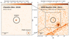 |
Fig. 1. Chandra (2018, left) and XMM-Newton (2021, right) full-band images of J1641+3755. The R = 5″ solid-line circle is centered on the optical position of the QSO. The dashed circle marks a field source. The dark stripe in the bottom right corner of the XMM-Newton image is an artifact due to a chip gap in the PN camera. Exposure times for the different instruments after removal of periods of high background are also reported. |
We analyzed the XMM-Newton photometry of J1641+3755 separately for the three EPIC cameras in the soft, hard, and full bands, following closely the procedure adopted by Vito et al. (2019). We extracted the source counts from a R = 15″ circular region centered on the optical position of J1641+3755, and the background counts from a nearby R = 30″ circular region, free of bright sources. The final results are not significantly affected by different choices of the extraction regions. We evaluated the detection significance using the binomial no-source probability PB of Weisskopf et al. (2007) and Broos et al. (2007). J1641+3755 is not detected significantly (i.e., we derived PB > 0.1) in any considered energy band by any individual camera.
Upper limits on the net counts were computed from the probability distribution functions (PDFs) of net counts following the method of Weisskopf et al. (2007) and they are reported in Table 2. Following Vito et al. (2019), we derived the PDFs of X-ray flux in the three energy bands from the net count-rate probability distribution function assuming a power-law spectrum with Γ = 2.05, accounting for Galactic absorption (Kalberla et al. 2005) and using the response matrices and PSF-corrected ancillary files extracted at the position of the QSO. Finally, for each energy band, we multiplied the flux PDFs of the three cameras and renormalized the resulting distribution to obtain the average flux PDF. We refer readers to Vito et al. (2019) for a discussion on this procedure. We derived upper limits on the flux in the three energy bands from the averaged PDFs (Table 3).
Derived X-ray properties of J1641+3755.
The rest-frame 2–10 keV band luminosity was computed from the unabsorbed fluxes in the soft band, assuming Γ = 2. We note that a basic analysis of the 2018 spectrum returned a steeper photon index than the value assumed here (Γ = 2.4 ± 0.5). However, the two values are consistent within the uncertainties, and the effect upon the derived flux is minor (see Tables 4 and 7 of Vito et al. 2019). Moreover, in the rest of the paper, we compare the X-ray properties derived from the 2018 and 2021 datasets consistently, assuming Γ = 2. The comparison between fluxes and luminosities derived from the two observation epochs quantitatively confirms that the X-ray emission of J1641+3755 varied significantly. We discuss this remarkable X-ray variability in Sect. 3.1.
2.2. LBT observation of J1641+3755
Triggered by the detection of the strong X-ray variability of J1641+3755 spanning over ≈115 rest-frame days, in March-May 2021 we carried out an LBT DDT program on this QSO quasi-simultaneously with the XMM-Newton observation (i.e., after 4 − 12 rest-frame days) to check if the rest-frame UV emission varied as well and to obtain a good quality rest-frame UV spectrum of J1641+3755. We used the Large Binocular Camera (LBC) to obtain imaging in the r and z bands (10 min on source) and both MODS and LUCI to cover the 5000 − 14 000 Å spectral range spectroscopically, including the expected positions of the Lyα and C IV emission lines, for 2 h on source per instrument. Table 4 summarizes the main LBT observation information.
Summary of the rest-frame UV observations of J1641+3755 with LBT.
2.2.1. LBC data reduction
Standard LBC reduction was carried out at the LBC Survey Center in Rome6, where individual exposures were combined with SWarp (Bertin et al. 2002) into stacked mosaic images, and astrometric and photometric calibrations, as well as the quality assessment, were performed with dedicated pipelines. We produced photometric catalogs using SExtractor (Bertin & Arnouts 1996), and performed object detection runs requiring a minimum number of nine connected pixels, each with a signal-to-noise ratio > 2σ, for a total detection significance of > 5σ for each object. We used the model-fitting photometry provided by SExtractor with the MAG_AUTO parameter.
2.2.2. MODS and LUCI data reductions
Standard MODS and LUCI reductions were carried out by the INAF LBT Spectroscopic Reduction Center in Milan7, where the LBT spectroscopic pipeline was developed (Scodeggio et al. 2005; Gargiulo et al. 2022). Relative flux calibration was obtained using a standard star for MODS and a telluric standard star for LUCI. We performed absolute flux calibration of the final spectra using the simultaneous photometric data obtained with LBT/LBC in the z band and LBT/LUCI in the J band. Finally, we smoothed the spectra with a Gaussian function with the standard deviation equal to the instrument wavelength resolutions.
3. Results
3.1. Variable X-ray emission
The X-ray flux declined by factors8 of > 6.6 in the soft and full bands, and by a factor of > 1.1 in the hard band between the 2018 and 2021 observing epochs (Table 3). The smaller variability limit in the hard band is due to the sensitivity limit of the XMM-Newton observations, which is shallower than in the soft and full band, and the large hard-band flux uncertainties, which are included in the estimate of the variability factor. In fact, the 2018 Chandra observation detected only ≈8 net counts in the hard band, compared to ≈40 and ≈50 net counts in the soft and full bands.
Fig. 2 presents the variability factor of J1641+3755 as a function of the rest-frame time separation between the two observation epochs, compared with other z > 6 QSOs observed in multiple epochs separated by more than ten rest-frame days (see Appendix A for details on this reference sample). We chose the time-separation threshold as a trade-off between collecting a statistically significant sample, and selecting objects with epoch separations similar to that of J1641+3755. We computed the variability factor as Fmax/Fmin, where Fmin and Fmax are the minimum and maximum full-band fluxes measured in two consecutive observation epochs, respectively. For consistency, we applied the same analysis to J1641+3755 and the reference QSO sample data.
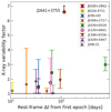 |
Fig. 2. Full-band X-ray variability factor between two consecutive observation epochs versus rest-frame time separation from the first epoch for z > 6 QSOs with multiple observations separated by more than ten rest-frame days. The only confirmed radio-loud objects among the considered QSOs are J0309+2717 and J1429+5447. Error bars factor in the flux uncertainties in the two epochs. |
J1641+3755 clearly shows strong X-ray variability compared to other high-redshift QSOs. In Sect. 4, we discuss some potential scenarios that could explain such a behavior. In addition to J1641, another QSO at z > 6, J1030+0524, is found to be significantly variable in the X-ray band, especially between observation epochs 2 and 3, when it varied by a factor of about three in ≈688 rest-frame days (see Appendix A). We refer readers to Nanni et al. (2018) for a thorough discussion of the variability properties of this object. All of the other QSOs reported in Fig. 2 are consistent with being nonvariable, or at most mildly variable by a factor of ≲2. Recently, Moretti et al. (2021) have reported significant flux (by a factor of ≈4 in the soft band) and a spectral variation in the z = 6.1 blazar J0309+2717 on rest-frame timescales of minutes, while in this work we focus on longer timescales.
As a consequence of the flux variability, the X-ray luminosity of J1641+3755 decreased from L2 − 10 keV ≈ 3 × 1045 erg s−1 to L2 − 10 keV ≲ 4 × 1044 erg s−1 (Table 3 and Fig. 3). The X-ray and bolometric luminosities of J1641+3755 in the two epochs are compared with those of other optically selected QSOs, and with the best-fitting relation of Duras et al. (2020) in Fig. 3. J1641+3755 was a significantly brighter X-ray source than QSOs with a similar bolometric luminosity in 2018, while its X-ray luminosity decreased to an X-ray normal, and possibly even weak, state in 2021.
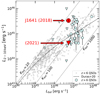 |
Fig. 3. X-ray luminosity versus bolometric luminosity for optically selected QSOs at z < 6 (collected from Lusso et al. 2012; Martocchia et al. 2017; Nanni et al. 2017; Salvestrini et al. 2019), and z > 6 QSOs (Connor et al. 2019, 2020; Vito et al. 2019, 2021; Pons et al. 2020; Wang et al. 2021a). Downward-pointing triangles represent upper limits for undetected objects. We used the updated value of Lbol for the 2021 epoch. The dashed black line represents the best-fitting relation of Duras et al. (2020). The location of J1641+3755 in 2018 and the upper limit in 2021 are marked in red. |
Timlin et al. (2020) show that only ≈1% of radio-quiet QSOs at all redshifts experience variability as dramatic as that seen from J1641, and this typically happens over longer timescales than what is probed for J1641. Moreover, the few extreme variability events known in QSOs can be linked with accretion physics beyond simple fluctuations of the accretion flow (see also, e.g., Ricci et al. 2020). For instance, recently Ni et al. (2020a) have presented extreme X-ray variability from a z = 1.9 weak-line QSO, which they interpret as an occultation event due to a thick inner accretion disk. Liu et al. (2019, 2021) report that a fraction of ≈15% of super-Eddington accreting QSOs, as J1641+3755 is (Table 1), are variable in the X-ray band by factors > 10. Since all such QSOs varied between X-ray normal and weak states, the authors propose that small-scale absorption can account for the flux variation. This interpretation does not explain the X-ray bright state of J1641+3755 in 2018 (see Sect. 4). Before J1641+3755, the most extreme X-ray variation in a z > 4 radio-quiet QSO was a factor of  in 74 rest-frame days for an object at z = 5.4 (Shemmer et al. 2005).
3.2. Variable rest-frame UV emission
From the 2021 LBT/LBC observations, we derived an AB magnitude zSDSS = 21.03 ± 0.03 for J1641+3755. In Fig. 4 we compare this value with the magnitudes derived from previous datasets. In particular, J1641+3755 is covered by the Canada France Hawaii Telescope (CFHT) Legacy Survey (CFHTLS)9, which was used to select it as a high-redshift QSO candidate originally (Willott et al. 2007). Moreover, J1641+3755 was detected by the PanSTARRS PS1 survey10 (e.g., Chambers et al. 2016) and the Mayall z-band Legacy Survey (MzLS; e.g., Dey et al. 2019)11. We downloaded the calibrated images and performed photometry with SExtractor using a consistent approach among the various datasets as described in Sect. 2.2.1. We calibrated the magnitudes using the public catalogs of the surveys12. The observation dates reported in Fig. 4 were taken directly from the headers of the files, except for PanSTARRS PS1, for which it is the median value of the individual images covering J1641+3755.
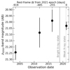 |
Fig. 4. Apparent magnitude in the z band as a function of the observation date. We compare our new LBT/LBC measurement in 2021, with magnitudes derived from the CFHT Legacy Survey, PanSTARRS PS1, and MzLS datasets (2003, 2011, and 2016, respectively). The solid vertical line marks the time of the 2018 Chandra observation, which detected bright X-ray emission from J1641+3755, while the dashed vertical line marks the time of the 2021 XMM-Newton observation that did not detect the QSO. |
In order to correct for the different z-band filters used to measure the QSO magnitudes in the various datasets, and thus be able to compare them fairly, we used the observed spectrum of J1641, which is presented in Sect. 3.3, to compute the offsets between the different filters. In particular, we convolved the spectrum with the z-band filters, obtaining synthetic magnitudes. The difference between the magnitude retrieved with the LBC filter and those obtained with the filters of the remaining facilities provided us with correction factors which we applied to the magnitudes measured from the CFHT, PanSTARRS, and MzLS datasets. The resulting magnitudes are in the LBC system, and they are reported in Fig. 4. This approach assumes that the spectral shape of J1641 has not varied significantly over the time baseline covered by the several datasets, as we discuss in Sect. 3.3. The final magnitudes of J1641+3755 corresponding to the LBC z-band filter are zSDSS = 21.24 ± 0.06, zSDSS = 21.09 ± 0.12, and zSDSS = 20.99 ± 0.09 for the CFHT, PanSTARRS, and MzLS datasets, respectively.
Using these four independent measurements13, we conclude that J1641+3755 has increased its rest-frame UV flux from 2003 to 2016 (i.e., over ≈2 rest-frame years) by ≈0.25 mag (Fig. 4), while no significant variation is found afterward. This behavior is the opposite of what we derived for the X-ray emission, although we note that the observation epochs before 2021 are very different among rest-frame UV and X-ray datasets. In particular, no rest-frame UV observation is available in 2018 (see solid vertical line in Fig. 4), when we detected bright X-ray emission from this QSO. Future observations of J1641 will reveal if its rest-frame UV emission remains constant or shows additional variability.
3.3. Rest-frame UV spectrum
Figure 5 presents the rest-frame UV spectrum of J1641+3755 obtained combining the LBT/MODS and LBT/LUCI observations. We measured a systemic redshift of z = 6.025 ± 0.002 based on the Si IV 1400 Å and C III] 1909 Å emission lines, which is slightly lower than the Willott et al. (2010) value of z = 6.047 ± 0.003 based on the Mg II 2798 Å emission line14.
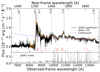 |
Fig. 5. Upper panel: combined LBT/MODS and LBT/LUCI spectra of J1641, smoothed with a Gaussian function with a standard deviation equal to the instrument wavelength resolutions (black line). We also show the composite spectrum of z > 5.7 QSOs of Shen et al. (2019, orange line), renormalized at rest-frame 1700 Å. The expected locations of emission lines at the measured redshift of J1641+3755 (i.e., 6.025) are marked as vertical dashed lines. The dashed violet line represents the best-fitting power-law continuum. Several narrow absorption lines are found in the spectrum: their locations are marked with short vertical ticks (see Table 5 and Fig. 6). We identified some of the absorption features with transitions due to an intervening system at z ≈ 5.67 (red ticks), while others are currently unidentified (gray ticks). Lower panel: error of the spectrum. |
The spectrum of J1641+3755 is broadly consistent with the composite spectrum of z > 5.7 QSOs of Shen et al. (2019). The spectral region at λ > 1.3 μm is at the red limit of the LBT/LUCI coverage, where the sensitivity drops and flux calibration becomes more uncertain. At those wavelengths, the difference between the J1641+3755 spectrum and the composite spectrum is larger.
Several narrow absorption lines are visible in the spectrum (see Table 5). Some of them are identified with atomic transitions consistent with a z = 5.67 intervening system and are marked with red vertical ticks in Fig. 5, while others are currently unidentified (gray vertical ticks). Fig. 6 zooms into the spectral ranges where the absorption features are detected, for a better visualization. The unidentified features may be due to absorbing material in the QSO rest frame, or one or more additional foreground systems. The emission “spikes" at wavelengths shorter than the Lyα emission line are probably due to the QSO radiation partially passing through the Lyα forest when it encounters regions along the line of sight with an increased ionized hydrogen fraction, which is possibly related to the presence of intervening ionizing sources, such as foreground galaxies.
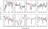 |
Fig. 6. Zooms into the portions of the J1641 spectrum where narrow absorption lines are detected (see Sect. 3.3 and Table 5). Transitions identified with an intervening system at z ≈ 5.67 are marked with vertical red lines, while unidentified lines are marked with vertical gray lines. Other apparent absorption features (e.g., in the second and third panels of the first row) are consistent with sky-line residuals. |
Narrow absorption features detected in the J1641+3755 rest-frame UV spectrum.
Assuming rest-frame continuum emission in the form of a simple power-law Fλ ∝ (λ/2500 Å)αλ, we fitted the wavelength range 11 730–12 645 Å, corresponding to rest-frame 1670–1800 Å, to retrieve the best-fitting UV spectral slope with a χ2 minimization method. We note that usually the UV spectral slope is fitted over several more wavelength intervals (e.g., Mazzucchelli et al. 2017), which are, however, affected by absorption features in the J1641+3755 spectrum, or out of the available spectroscopic coverage. Following Shen et al. (2019) and Yang et al. (2021), for example, we used a Monte Carlo approach to estimate the uncertainties: we generated a set of 100 mock spectra by perturbing the original spectrum at each pixel with random Gaussian noise with the standard deviation being set equal to the spectral uncertainty at that pixel. Then, we estimated the uncertainties on the parameter values as the 16% and 84% percentile of the final best-fitting value distribution. We derived a best-fitting  (dotted purple line in Fig. 5). Due to the limited “leverage” provided by the fitted wavelength range, the uncertainties are large and the best-fitting value itself is quite sensitive to the exact wavelength interval used in the fitting.
We also fit the C IV emission line, assuming a more complex model that simultaneously includes, in addition to the intrinsic continuum, the Balmer pseudo-continuum modeled as in Schindler et al. (2020), the iron pseudo-continuum template of Vestergaard & Wilkes (2001), and a Gaussian function for the C IV line (Fig. 7). To be consistent with previous literature works (e.g., Mazzucchelli et al. 2017; Schindler et al. 2020; Vito et al. 2021), we convolved the iron pseudo-continuum model with a Gaussian function with the width being equal to that of the Mg II emission line. Since that line is not covered by our spectrum, we assumed the width reported by Willott et al. (2010)15. We performed the fit in the rest-frame wavelength ranges 1480–1590 Å and 1670–1800 Å. We obtained a best-fitting  , while the C IV emission line is centered at
  (i.e., zCIV = 6.000 ± 0.002), corresponding to a blueshift of ≈ − 1100 km s−1 from the systemic redshift, with
  and rest-frame equivalent width
  . These values are consistent with typical measurements reported for z ≳ 6 QSOs (e.g., Shen et al. 2019; Schindler et al. 2020; Yang et al. 2021), and with the prescription of Dix et al. (2020), which links the blueshift, FWHM, and equivalent width (EW) of the C IV emission line with the UV luminosity of a QSO.
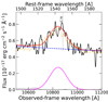 |
Fig. 7. Observed spectrum of the C IV emission-line region (black line) and best-fitting model (red line). The best-fitting individual components are also shown: the dashed blue line is the combined intrinsic continuum and Balmer pseudo-continuum model; the magenta line is the Gaussian component; and the gray line is the iron pseudo-continuum. For reference, the orange line represents the composite spectrum of z > 5.7 QSOs of Shen et al. (2019), and the vertical dashed line marks the expected location of the C IV emission line assuming the systemic redshift of z = 6.025. The observed blueshift of ≈1000 km s−1 is consistent with typical values of z > 6 QSOs. |
In Fig. 8, we compare the 2021 LBT spectrum of J1641+3755 with a 2007 Keck/ESI spectrum16 covering the 4000–9300 Å range, which was presented by Willott et al. (2007) and Eilers et al. (2018), and normalized at rest-frame 9000 Å17. The two spectra are broadly consistent in terms of the spectral shape, the Lyα and N V emission-line complex, and the presence of several narrow absorption features at 8500–9000 Å, suggesting that the rest-frame UV variability discussed in Sect. 3.2 is not due to a variation in the spectral shape, at least in this relatively narrow wavelength range.
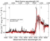 |
Fig. 8. LBT rest-frame UV spectrum of J1641+3755 in 2021 (black line), compared with the (renormalized) Keck spectrum presented by Willott et al. (2007) and Eilers et al. (2018). The overall spectral shape, as well as the emission and absorption features in the overlapping spectral range are broadly consistent between the two epochs. |
4. Discussion
4.1. Possible causes for the variability of J1641+3755
Any physical interpretation of the variability properties of J1641+3755 should address both the fading of the X-ray emission over a rest-frame period of 115 days (Sect. 3.1), corresponding to a light-crossing distance d < ct ≈ 0.1 pc, which is comparable to the size of a QSO accretion disk, and the QSO brightening in the rest-frame UV band (Sect. 3.2). Ideally, any interpretation should explain the fact that in 2018, J1641+3755 was a ≈2σ positive outlier from the LX − Lbol and αox − LUV relations (Vito et al. 2019; see, e.g., Fig. 3)18. However, there is an additional complication due to the nonsimultaneity of the rest-frame UV and X-ray observations (see Table 2 and Fig. 4).
The variability of J1641+3755 can be a result of intrinsic or extrinsic physical effects. Here we discuss some possible explanations involving intrinsic mechanisms. According to standard accretion physics, a drop in the SMBH accretion rate19 should have produced a decrease in the rest-frame UV emission, in addition to the drop in the X-ray flux (e.g., LaMassa et al. 2015). However, our LBC observations reveal that between 2016 and 2021, the QSO did not vary its rest-frame UV magnitude significantly, and it was brighter than in previous epochs. This tension may be due to the nonsimultaneity of the X-ray and UV observation epochs before 2021, as the bright X-ray state in 2018 could correspond to a bright UV state, which, however, might not have been detected due to the lack of simultaneous UV observations. Alternatively, the 2018 X-ray epoch could correspond to a strong and short local maximum of a long-term fading X-ray light curve, as QSO variability timescales are generally shorter in the X-rays than in the UV band. However, as discussed in Sect. 3.1, such a strong X-ray variability event on short timescales is remarkably rare for a luminous QSO.
On the other hand, some models predict a brightening of the rest-frame UV emission and a suppression of X-ray emission for increasing accretion rates (e.g., Giustini & Proga 2019). This behavior is usually associated with the launching of strong and fast nuclear winds, for which, however, we do not find definitive evidence in Fig. 5.
Finally, intervening heavy obscuration on spatial scales comparable with the inner accretion disk could completely screen the X-ray emission, leaving the rest-frame UV unaffected. For instance, models of super-Eddington accretion predict the presence of a geometrically thick inner disk (e.g., Wang et al. 2014; Jiang et al. 2019). In this case, a change in the disk thickness (e.g., due to disk rotation or variation in the accretion rate) can produce the X-ray variability observed for J1641+3755, similarly to the event discussed by Ni et al. (2020a, 2022), while an increase in the accretion rate would account for the UV brightening.
All of the aforementioned possibilities describe the X-ray variability of J1641+3755 well, but they rely on a secondary effect to explain why its X-ray luminosity in 2018 was significantly higher than the expectation from the LX − LUV relation. In particular, they require an undetected bright UV state in 2018 due to the lack of UV observations, or that the 2018 X-ray emission was produced by an extreme and rare burst.
Possible extrinsic effects account, more easily, for the J1641+3755 variability properties and its apparent bright X-ray state in 2018. For instance, J1641+3755 may be an intrinsically low-luminosity QSO, whose emission is boosted by gravitational lensing due to a foreground object or structure, similarly to the first lensed z > 6 QSO recently discovered by Fan et al. (2019). A modest magnification factor (≈5 − 10) would bring the 2018 luminosity back to the expected relation between Lx and LUV. In this context, the strong X-ray flux variation can be intrinsic, as QSO variability amplitude is generally found to increase for decreasing luminosity (e.g., Shemmer et al. 2017), due to a small-scale obscuration event in 2021 (e.g., Liu et al. 2019; Ni et al. 2020b), or due to microlensing effects. In fact, microlensing due to the stars in a lens galaxy aligned with a QSO can produce observed flux variability in addition to intrinsic variability (e.g., Chen et al. 2012; MacLeod et al. 2015), affecting X-ray emission in particular (e.g., Chartas et al. 2002, 2016; Popovic et al. 2006), which is produced in a compact region close to the SMBH. Timescales for X-ray emission variations induced by microlensing are as short as months (e.g., Jovanović et al. 2008), depending on the geometry of the system.
Another possibility involving an extrinsic mechanism is that the X-ray luminosity measured in 2021 is the correct value for J1641, and the X-ray emission detected in 2018 has been produced by a transient event – for example, a tidal disruption event, (TDE) – in an unidentified foreground object. In this case, the UV brightening can be related to a small variation in the QSO accretion rate. The SMBH powering J1641+3755 could not produce a TDE, since, given its mass (Table 1), it would have directly accreted a nearby star rather than tidally disrupted it (e.g., Kesden 2012; Komossa 2015).
The last two hypotheses require the presence of a foreground galaxy at a small projected distance (e.g., ≲1″ in the case of a foreground TDE) from the QSO. Evidence for the possible presence of foreground galaxies and structures in the direction of J1641+3755 are discussed in Sect. 3.3. For instance, the narrow absorption lines in the spectrum of J1641+3755 could be due to absorption by a foreground object, and a number of them are consistent with an intervening system at z = 5.67. Moreover, the MODS spectrum shows emission peaks blueward of the Lyα line, which are due to completely ionized regions along the QSO direction, possibly related to the presence of some sources of ionizing radiation.
4.2. Possible enhanced X-ray variability in high-redshift QSOs
Out of ten QSOs at z > 6 covered with multi-epoch X-ray data (set to Δt > 10 rest-frame days), at least two (J1641+3755 and J1030+0524; i.e., 20%) present significant X-ray variability (i.e., by a factor of ≳3; see Fig. 2). The incidence of X-ray variable QSOs at high redshift increases if radio-loud objects (i.e., J0309+2717 and J1429+5447) are excluded. For comparison, Timlin et al. (2020, see their Fig. 8) found that a variability amplitude by a factor of ≳3 is detected for < 10% of the general radio-quiet QSO population. Such a fraction decreases if QSOs, with observation epochs separated by timescales similar to that of J1641+3755 or with similar luminosities to J1641+3755, are considered (Figs. 7 and 8 of Timlin et al. 2020). In fact, z > 6 QSOs are typically luminous systems, which at later cosmic times are usually found to be less variable than low-luminosity objects (e.g., Shemmer et al. 2017; Thomas et al. 2021).
This finding suggests that enhanced variability may be a characteristic property of high-redshift QSOs, which is perhaps linked with the physics of the fast accretion rate required to grow to 109 M⊙ in a few hundred million years. In fact, the incidence of extreme variability events has been found to correlate with the Eddington ratio (e.g., Miniutti et al. 2012; Liu et al. 2019, 2021; Ni et al. 2020a, 2022), and the accretion rates of known z ≈ 6 QSOs are typically close to the Eddington limit. Multi-epoch X-ray observations of high-redshift QSOs with current (e.g., the XMM-Newton Multi-Year Heritage Programme Hyperion; PI: L. Zappacosta) and future (e.g., Marchesi et al. 2020) facilities are required to confirm this hypothesis since, for instance, QSOs at z ≈ 4 do not obviously present such an enhancement compared with the general population at lower redshift (e.g., Lanzuisi et al. 2014; Shemmer et al. 2017).
5. Conclusions and future prospects
We have presented quasi-simultaneous X-ray and rest-frame UV observations of the z = 6.025 QSO J1641, which was already observed in both bands in previous epochs. Here, we summarize the main conclusions:
-
We did not detect J1641+3755 in a 100 ks XMM-Newton observation performed in 2021. The comparison with a 2018 (i.e., 115 rest-frame days before) Chandra observation, which detected J1641+3755 as a luminous QSO, reveals that the X-ray emission from this object dropped by a factor ≳7, which is the most extreme one witnessed in a z > 4 QSO (Shemmer et al. 2005). Timlin et al. (2020) show that only ≈1% of the general QSO population has been found to experience such a strong variation, and typically on much longer timescales.
-
Two QSOs (J1641+3755 and J1030+0524) out of the ten QSOs at z > 6 observed in the X-ray band in multiple epochs separated by more than ten rest-frame days and detected in at least one epoch are found to be strongly variable (i.e., by a factor > 3). This fraction is higher than that observed at lower redshift (i.e., < 10%), although its statistical significance is poor due to the limited sample size. Enhanced variability can be a characteristic property of high-redshift QSOs, possibly linked with the physics of fast accretion required to form ≳109 M⊙ SMBHs at z > 6. Future X-ray observations of high-redshift QSOs will confirm this hypothesis.
-
A four-epoch rest-frame UV light curve of J1641+3755 revealed that it became brighter by ≈0.25 mag from 2003 to 2016, whereas it did not vary significantly afterward. This behavior is opposite to what we found for the X-ray emission. However, observations in the two bands before 2021 were performed nonsimultaneously, hindering a clear physical interpretation.
-
The rest-frame UV continuum and emission-line properties of J1641+3755 are consistent with what is found for the general population of high-redshift QSOs. However, several narrow absorption lines are detected as well, and a number of them are consistent with transitions due to an intervening system at z = 5.67.
-
We have discussed a number of possible physical explanations for the remarkable variability properties of J1641, including intrinsic and extrinsic causes. The former causes include a variation in the accretion rate, possibly coupled with absorption due to outflowing material or a thick accretion disk. Among the latter is gravitational lensing, which would imply that J1641+3755 is intrinsically less luminous than what appears, alleviating the tension between its luminosity and strong variability. The bright X-ray emission in 2018, when J1641+3755 was a 2σ outlier from known relations between LX and LUV, is the most difficult result to explain with these scenarios. A possibility is that it was due to a foreground event (e.g., a tidal disruption event) not physically associated with J1641.
Monitoring observations of J1641+3755 will allow us to follow and constrain its variability behavior better. In particular, we have recently secured a multicycle Chandra program to follow-up on J1641+3755 and test if it returns to a bright X-ray state, or to place tighter constraints on its current X-ray luminosity. Additional LBT/LBC observations will confirm the UV brightening of J1641+3755. An important aspect is to obtain quasi-simultaneous X-ray and rest-frame UV data to check if the UV emission indeed follows the opposite trend as the X-ray variability, or if that finding was due to the different time baselines probed in the two bands in this work. The results will help the physical interpretation of the variability properties of J1641+3755, considering the several possible causes we have discussed.
This QSO has R < 10 (Vito et al. 2019), where R = fν, 5 GHz/fν, 4400 Å is the radio-loudness parameter, i.e., the ratio of the flux densities at rest-frame 5 GHz and 4400 Å (e.g., Kellermann et al. 1989).
The quantity αox = 0.384 × (log L2 keV − log L2500 Å) is well known to anticorrelate with L2500 Å (e.g., Steffen et al. 2006; Just et al. 2007; Lusso & Risaliti 2016, 2017). This relation does not significantly change up to z ≈ 7 (e.g., Vito et al. 2019; Wang et al. 2021a). We define Δαox = αox(obs)−αox(exp), where αox(obs) is the observed value and αox(exp) is the value expected at a given L2500 Å.
This value is consistent with the average photon index of luminous QSOs (e.g., Shemmer et al. 2006; Nanni et al. 2017), and it is the value used in Vito et al. (2019).
We conservatively compare the lower boundaries of the 2018 flux intervals reported in Table 3 with the 2021 flux upper limits.
While the Mg II emission line is generally considered a more accurate systemic redshift indicator than the Si IV and C III] lines (e.g., Shen et al. 2016), it is close to the border of the Willott et al. (2010) noisy spectrum, where uncertainties are high.
We retrieved this spectrum from the igmspec database (Prochaska 2017, see also Sect. 2.4 of Eilers et al. 2018): https://specdb.readthedocs.io/en/latest/igmspec.html.
The absolute flux calibration of the Keck and LBT spectra is based on the CFHT and LBT/LBC photometry, respectively, and thus is affected by the UV variability discussed in Sect. 3.2.
We note that the viscous timescale tvis (i.e., the typical timescale on which the accretion rate varies) of a standard geometrically thin accretion disk for MBH ≈ 108 M⊙ is longer than the observed ≈115 day variation time. However, for BHs accreting at super-Eddington rates, as is likely J1641+3755, the accretion disk might be geometrically thick (e.g., Wang et al. 2014; Jiang et al. 2019). In this case, tvis decreases sharply below the observed variability timescale (e.g., Czerny 2006; Fabrika et al. 2021). Therefore, we cannot discard a variation in the accretion rate as the cause for the observed variability of J1641+3755 using timescale arguments.
Acknowledgments
We thank the anonymous referee for the useful comments that improved the paper. We thank S. Carniani for useful discussion. W.N.B. thanks support from NASA grant 80NSSC20K0795 and the V.M. Willaman Endowment. F.E.B. acknowledges support from ANID-Chile BASAL AFB-170002, ACE210002, and FB210003, FONDECYT Regular 1200495 and 1190818, and Millennium Science Initiative Program – ICN12_009. S.M. acknowledges funding from the INAF Progetti di Ricerca di Rilevante Interesse Nazionale (PRIN), Bando 2019 (project: “Piercing through the clouds: a multiwavelength study of obscured accretion in nearby supermassive black holes”). B.L. acknowledges financial support from the National Natural Science Foundation of China grant 11991053. We acknowledge the support from the LBT-Italian Coordination Facility for the execution of observations, data distribution and reduction. The LBT is an international collaboration among institutions in the United States, Italy and Germany. LBT Corporation partners are: The University of Arizona on behalf of the Arizona university system; Istituto Nazionale di Astrofisica, Italy; LBT Beteiligungsgesellschaft, Germany, representing the Max-Planck Society, the Astrophysical Institute Potsdam, and Heidelberg University; The Ohio State University, and The Research Corporation, on behalf of The University of Notre Dame, University of Minnesota and University of Virginia. This research has made use of data obtained from the Chandra Data Archive (Proposal ID 19700183), and software provided by the Chandra X-ray Center (CXC) in the application packages CIAO. Based on observations obtained with XMM-Newton, an ESA science mission with instruments and contributions directly funded by ESA Member States and NASA The Mayall z-band Legacy Survey (MzLS; NOAO Prop. ID # 2016A-0453; PI: A. Dey) uses observations made with the Mosaic-3 camera at the Mayall 4m telescope at Kitt Peak National Observatory, National Optical Astronomy Observatory, which is operated by the Association of Universities for Research in Astronomy (AURA) under cooperative agreement with the National Science Foundation. The authors are honored to be permitted to conduct astronomical research on Iolkam Du’ag (Kitt Peak), a mountain with particular significance to the Tohono O’odham. The Pan-STARRS1 Surveys (PS1) and the PS1 public science archive have been made possible through contributions by the Institute for Astronomy, the University of Hawaii, the Pan-STARRS Project Office, the Max-Planck Society and its participating institutes, the Max Planck Institute for Astronomy, Heidelberg and the Max Planck Institute for Extraterrestrial Physics, Garching, The Johns Hopkins University, Durham University, the University of Edinburgh, the Queen’s University Belfast, the Harvard-Smithsonian Center for Astrophysics, the Las Cumbres Observatory Global Telescope Network Incorporated, the National Central University of Taiwan, the Space Telescope Science Institute, the National Aeronautics and Space Administration under Grant No. NNX08AR22G issued through the Planetary Science Division of the NASA Science Mission Directorate, the National Science Foundation Grant No. AST-1238877, the University of Maryland, Eotvos Lorand University (ELTE), the Los Alamos National Laboratory, and the Gordon and Betty Moore Foundation. Based on observations obtained with MegaPrime/MegaCam, a joint project of CFHT and CEA/IRFU, at the Canada-France-Hawaii Telescope (CFHT) which is operated by the National Research Council (NRC) of Canada, the Institut National des Science de l’Univers of the Centre National de la Recherche Scientifique (CNRS) of France, and the University of Hawaii. This work is based in part on data products produced at Terapix available at the Canadian Astronomy Data Centre as part of the Canada-France-Hawaii Telescope Legacy Survey, a collaborative project of NRC and CNRS. This research used the facilities of the Canadian Astronomy Data Centre operated by the National Research Council of Canada with the support of the Canadian Space Agency. This research made use of APLpy, an open-source plotting package for Python hosted at https://aplpy.github.io/. This research made use of Astropy, a community-developed core Python package for Astronomy (Astropy Collaboration 2013, 2018).
References
- Ai, Y., Dou, L., Fan, X., et al. 2016, ApJ, 823, L37 [Google Scholar]
- Ai, Y., Fabian, A. C., Fan, X., et al. 2017, MNRAS, 470, 1587 [NASA ADS] [CrossRef] [Google Scholar]
- Astropy Collaboration (Robitaille, T. P., et al.) 2013, A&A, 558, A33 [NASA ADS] [CrossRef] [EDP Sciences] [Google Scholar]
- Astropy Collaboration (Price-Whelan, A. M., et al.) 2018, AJ, 156, 123 [Google Scholar]
- Bañados, E., Venemans, B. P., Morganson, E., et al. 2015, ApJ, 804, 118 [Google Scholar]
- Bañados, E., Venemans, B. P., Decarli, R., et al. 2016, ApJS, 227, 11 [Google Scholar]
- Bañados, E., Venemans, B. P., Mazzucchelli, C., et al. 2018, Nature, 553, 473 [Google Scholar]
- Belladitta, S., Moretti, A., Caccianiga, A., et al. 2020, A&A, 635, L7 [EDP Sciences] [Google Scholar]
- Bertin, E., & Arnouts, S. 1996, A&AS, 117, 393 [NASA ADS] [CrossRef] [EDP Sciences] [Google Scholar]
- Bertin, E., Mellier, Y., Radovich, M., et al. 2002, in Astronomical Data Analysis Software and Systems XI, eds. D. A. Bohlender, D. Durand, & T. H. Handley, ASP Conf. Ser., 281, 228 [NASA ADS] [Google Scholar]
- Brandt, W. N., Schneider, D. P., Fan, X., et al. 2002, ApJ, 569, L5 [Google Scholar]
- Brightman, M., Silverman, J. D., Mainieri, V., et al. 2013, MNRAS, 433, 2485 [Google Scholar]
- Broos, P. S., Feigelson, E. D., Townsley, L. K., et al. 2007, ApJS, 169, 353 [Google Scholar]
- Castelló-Mor, N., Kaspi, S., Netzer, H., et al. 2017, MNRAS, 467, 1209 [NASA ADS] [Google Scholar]
- Chambers, K. C., Magnier, E. A., Metcalfe, N., et al. 2016, ArXiv e-prints [arXiv:1612.05560] [Google Scholar]
- Chartas, G., Agol, E., Eracleous, M., et al. 2002, ApJ, 568, 509 [NASA ADS] [CrossRef] [Google Scholar]
- Chartas, G., Rhea, C., Kochanek, C., et al. 2016, Astron. Nachr., 337, 356 [NASA ADS] [CrossRef] [Google Scholar]
- Chen, B., Dai, X., Kochanek, C. S., et al. 2012, ApJ, 755, 24 [Google Scholar]
- Connor, T., Bañados, E., Stern, D., et al. 2019, ApJ, 887, 171 [Google Scholar]
- Connor, T., Bañados, E., Mazzucchelli, C., et al. 2020, ApJ, 900, 189 [Google Scholar]
- Czerny, B. 2006, in AGN Variability from X-Rays to Radio Waves, eds. C. M. Gaskell, I. M. McHardy, B. M. Peterson, & S. G. Sergeev, ASP Conf. Ser., 360, 265 [NASA ADS] [Google Scholar]
- Decarli, R., Walter, F., Venemans, B. P., et al. 2018, ApJ, 854, 97 [Google Scholar]
- De Rosa, G., Venemans, B. P., Decarli, R., et al. 2014, ApJ, 790, 145 [Google Scholar]
- Dey, A., Schlegel, D. J., Lang, D., et al. 2019, AJ, 157, 168 [Google Scholar]
- Dix, C., Shemmer, O., Brotherton, M. S., et al. 2020, ApJ, 893, 14 [NASA ADS] [CrossRef] [Google Scholar]
- Duras, F., Bongiorno, A., Ricci, F., et al. 2020, A&A, 636, A73 [NASA ADS] [CrossRef] [EDP Sciences] [Google Scholar]
- Eilers, A.-C., Davies, F. B., & Hennawi, J. F. 2018, ApJ, 864, 53 [NASA ADS] [CrossRef] [Google Scholar]
- Fabrika, S. N., Atapin, K. E., Vinokurov, A. S., & Sholukhova, O. N. 2021, Astrophys. Bull., 76, 6 [NASA ADS] [CrossRef] [Google Scholar]
- Fan, X., Narayanan, V. K., Lupton, R. H., et al. 2001, AJ, 122, 2833 [Google Scholar]
- Fan, X., Wang, F., Yang, J., et al. 2019, ApJ, 870, L11 [Google Scholar]
- Farrah, D., Priddey, R., Wilman, R., Haehnelt, M., & McMahon, R. 2004, ApJ, 611, L13 [NASA ADS] [CrossRef] [Google Scholar]
- Gargiulo, A., Fumana, M., Bisogni, S., et al. 2022, MNRAS, 514, 2902 [NASA ADS] [CrossRef] [Google Scholar]
- Gibson, R. R., & Brandt, W. N. 2012, ApJ, 746, 54 [NASA ADS] [CrossRef] [Google Scholar]
- Giustini, M., & Proga, D. 2019, A&A, 630, A94 [NASA ADS] [CrossRef] [EDP Sciences] [Google Scholar]
- Ighina, L., Moretti, A., Tavecchio, F., et al. 2022, A&A, 659, A93 [NASA ADS] [CrossRef] [EDP Sciences] [Google Scholar]
- Jiang, Y.-F., Stone, J. M., & Davis, S. W. 2019, ApJ, 880, 67 [Google Scholar]
- Jovanović, P., Zakharov, A. F., Popović, L. Č., & Petrović, T. 2008, MNRAS, 386, 397 [Google Scholar]
- Just, D. W., Brandt, W. N., Shemmer, O., et al. 2007, ApJ, 665, 1004 [Google Scholar]
- Kalberla, P. M. W., Burton, W. B., Hartmann, D., et al. 2005, A&A, 440, 775 [NASA ADS] [CrossRef] [EDP Sciences] [Google Scholar]
- Kellermann, K. I., Sramek, R., Schmidt, M., Shaffer, D. B., & Green, R. 1989, AJ, 98, 1195 [Google Scholar]
- Kesden, M. 2012, Phys. Rev. D, 85, 024037 [NASA ADS] [CrossRef] [Google Scholar]
- Komossa, S. 2015, J. High Energy Astrophys., 7, 148 [Google Scholar]
- Kurk, J. D., Walter, F., Fan, X., et al. 2007, ApJ, 669, 32 [NASA ADS] [CrossRef] [Google Scholar]
- LaMassa, S. M., Cales, S., Moran, E. C., et al. 2015, ApJ, 800, 144 [NASA ADS] [CrossRef] [Google Scholar]
- Lanzuisi, G., Ponti, G., Salvato, M., et al. 2014, ApJ, 781, 105 [NASA ADS] [CrossRef] [Google Scholar]
- Liu, H., Luo, B., Brandt, W. N., et al. 2019, ApJ, 878, 79 [NASA ADS] [CrossRef] [Google Scholar]
- Liu, H., Luo, B., Brandt, W. N., et al. 2021, ApJ, 910, 103 [Google Scholar]
- Luo, B., Brandt, W. N., Hall, P. B., et al. 2015, ApJ, 805, 122 [Google Scholar]
- Lusso, E., & Risaliti, G. 2016, ApJ, 819, 154 [Google Scholar]
- Lusso, E., & Risaliti, G. 2017, A&A, 602, A79 [NASA ADS] [CrossRef] [EDP Sciences] [Google Scholar]
- Lusso, E., Comastri, A., Simmons, B. D., et al. 2012, MNRAS, 425, 623 [Google Scholar]
- MacLeod, C. L., Morgan, C. W., Mosquera, A., et al. 2015, ApJ, 806, 258 [NASA ADS] [CrossRef] [Google Scholar]
- Marchesi, S., Gilli, R., Lanzuisi, G., et al. 2020, A&A, 642, A184 [EDP Sciences] [Google Scholar]
- Martocchia, S., Piconcelli, E., Zappacosta, L., et al. 2017, A&A, 608, A51 [NASA ADS] [CrossRef] [EDP Sciences] [Google Scholar]
- Matsuoka, Y., Iwasawa, K., Onoue, M., et al. 2022, ApJS, 259, 18 [NASA ADS] [CrossRef] [Google Scholar]
- Mazzucchelli, C., Bañados, E., Venemans, B. P., et al. 2017, ApJ, 849, 91 [Google Scholar]
- Medvedev, P., Sazonov, S., Gilfanov, M., et al. 2020, MNRAS, 497, 1842 [Google Scholar]
- Medvedev, P., Gilfanov, M., Sazonov, S., Schartel, N., & Sunyaev, R. 2021, MNRAS, 504, 576 [CrossRef] [Google Scholar]
- Meier, D. L. 2012, Black Hole Astrophysics: The Engine Paradigm (Verlag Berlin Heidelberg: Springer) [Google Scholar]
- Meyer, R. A., Bosman, S. E. I., & Ellis, R. S. 2019, MNRAS, 487, 3305 [Google Scholar]
- Middei, R., Vagnetti, F., Bianchi, S., et al. 2017, A&A, 599, A82 [NASA ADS] [CrossRef] [EDP Sciences] [Google Scholar]
- Miniutti, G., Brandt, W. N., Schneider, D. P., et al. 2012, MNRAS, 425, 1718 [NASA ADS] [CrossRef] [Google Scholar]
- Moretti, A., Ballo, L., Braito, V., et al. 2014, A&A, 563, A46 [NASA ADS] [CrossRef] [EDP Sciences] [Google Scholar]
- Moretti, A., Ghisellini, G., Caccianiga, A., et al. 2021, ApJ, 920, 15 [NASA ADS] [CrossRef] [Google Scholar]
- Nanni, R., Vignali, C., Gilli, R., Moretti, A., & Brandt, W. N. 2017, A&A, 603, A128 [NASA ADS] [CrossRef] [EDP Sciences] [Google Scholar]
- Nanni, R., Gilli, R., Vignali, C., et al. 2018, A&A, 614, A121 [NASA ADS] [CrossRef] [EDP Sciences] [Google Scholar]
- Ni, Q., Brandt, W. N., Yi, W., et al. 2020a, ApJ, 889, L37 [NASA ADS] [CrossRef] [Google Scholar]
- Ni, Y., Di Matteo, T., Gilli, R., et al. 2020b, MNRAS, 495, 2135 [NASA ADS] [CrossRef] [Google Scholar]
- Ni, Q., Brandt, W. N., Luo, B., et al. 2022, MNRAS, 511, 5251 [NASA ADS] [CrossRef] [Google Scholar]
- Paolillo, M., Papadakis, I., Brandt, W. N., et al. 2017, MNRAS, 471, 4398 [Google Scholar]
- Planck Collaboration XIII. 2016, A&A, 594, A13 [NASA ADS] [CrossRef] [EDP Sciences] [Google Scholar]
- Pons, E., McMahon, R. G., Banerji, M., & Reed, S. L. 2020, MNRAS, 491, 3884 [Google Scholar]
- Popovic, L. C., Jovanovic, P., Petrovic, T., & Shalyapin, V. N. 2006, Astron. Nachr., 327, 981 [NASA ADS] [CrossRef] [Google Scholar]
- Prochaska, J. X. 2017, Astron. Comput., 19, 27 [NASA ADS] [CrossRef] [Google Scholar]
- Reines, A. E., & Comastri, A. 2016, PASA, 33 [CrossRef] [Google Scholar]
- Ricci, C., Kara, E., Loewenstein, M., et al. 2020, ApJ, 898, L1 [Google Scholar]
- Salvestrini, F., Risaliti, G., Bisogni, S., Lusso, E., & Vignali, C. 2019, A&A, 631, A120 [NASA ADS] [CrossRef] [EDP Sciences] [Google Scholar]
- Schindler, J.-T., Farina, E. P., Bañados, E., et al. 2020, ApJ, 905, 51 [Google Scholar]
- Schwartz, D. A., & Virani, S. N. 2004, ApJ, 615, L21 [NASA ADS] [CrossRef] [Google Scholar]
- Scodeggio, M., Franzetti, P., Garilli, B., et al. 2005, PASP, 117, 1284 [NASA ADS] [CrossRef] [Google Scholar]
- Shemmer, O., Brandt, W. N., Vignali, C., et al. 2005, ApJ, 630, 729 [Google Scholar]
- Shemmer, O., Brandt, W. N., Netzer, H., Maiolino, R., & Kaspi, S. 2006, ApJ, 646, L29 [Google Scholar]
- Shemmer, O., Brandt, W. N., Paolillo, M., et al. 2017, ApJ, 848, 46 [Google Scholar]
- Shen, Y., Brandt, W. N., Richards, G. T., et al. 2016, ApJ, 831, 7 [NASA ADS] [CrossRef] [Google Scholar]
- Shen, Y., Wu, J., Jiang, L., et al. 2019, ApJ, 873, 35 [Google Scholar]
- Steffen, A. T., Strateva, I., Brandt, W. N., et al. 2006, AJ, 131, 2826 [Google Scholar]
- Thomas, M. O., Shemmer, O., Brandt, W. N., et al. 2021, ApJ, 923, 111 [NASA ADS] [CrossRef] [Google Scholar]
- Timlin, J. D. I., Brandt, W. N., Zhu, S., et al. 2020, MNRAS, 498, 4033 [Google Scholar]
- Vagnetti, F., Middei, R., Antonucci, M., Paolillo, M., & Serafinelli, R. 2016, A&A, 593, A55 [NASA ADS] [CrossRef] [EDP Sciences] [Google Scholar]
- Venemans, B. P., McMahon, R. G., Walter, F., et al. 2012, ApJ, 751, L25 [NASA ADS] [CrossRef] [Google Scholar]
- Venemans, B. P., Walter, F., Zschaechner, L., et al. 2016, ApJ, 816, 37 [Google Scholar]
- Vestergaard, M., & Wilkes, B. J. 2001, ApJS, 134, 1 [Google Scholar]
- Vito, F., Brandt, W. N., Bauer, F. E., et al. 2019, A&A, 630, A118 [NASA ADS] [CrossRef] [EDP Sciences] [Google Scholar]
- Vito, F., Brandt, W. N., Ricci, F., et al. 2021, A&A, 649, A133 [NASA ADS] [CrossRef] [EDP Sciences] [Google Scholar]
- Wang, R., Wagg, J., Carilli, C. L., et al. 2011, ApJ, 739, L34 [Google Scholar]
- Wang, J.-M., Qiu, J., Du, P., & Ho, L. C. 2014, ApJ, 797, 65 [NASA ADS] [CrossRef] [Google Scholar]
- Wang, R., Wu, X.-B., Neri, R., et al. 2016, ApJ, 830, 53 [Google Scholar]
- Wang, F., Yang, J., Fan, X., et al. 2021a, ApJ, 907, L1 [Google Scholar]
- Wang, F., Fan, X., Yang, J., et al. 2021b, ApJ, 908, 53 [Google Scholar]
- Webb, N. A., Coriat, M., Traulsen, I., et al. 2020, A&A, 641, A136 [NASA ADS] [CrossRef] [EDP Sciences] [Google Scholar]
- Weisskopf, M. C., Wu, K., Trimble, V., et al. 2007, ApJ, 657, 1026 [Google Scholar]
- Willott, C. J., Delorme, P., Omont, A., et al. 2007, AJ, 134, 2435 [NASA ADS] [CrossRef] [Google Scholar]
- Willott, C. J., Albert, L., Arzoumanian, D., et al. 2010, AJ, 140, 546 [NASA ADS] [CrossRef] [Google Scholar]
- Woods, T. E., Agarwal, B., Bromm, V., et al. 2019, PASA, 36 [Google Scholar]
- Wu, X.-B., Wang, F., Fan, X., et al. 2015, Nature, 518, 512 [Google Scholar]
- Yang, J., Wang, F., Fan, X., et al. 2021, ApJ, 923, 262 [NASA ADS] [CrossRef] [Google Scholar]
Appendix A: Sample of z > 6 QSOs with multiple-epoch X-ray observations
We collected a sample of ten QSOs at z > 6 covered with X-ray observations in multiple epochs separated by more than ten rest-frame days (Tab. A.1). All of these QSOs are not bright radio sources, except for the radio-loud QSOs J0309+2717 and J1429+5447. We grouped observations performed within ten rest-frame days in an individual epoch, with the exception of J1030+0524. This QSO was observed in 2017 with a Chandra Large Program (Nanni et al. 2018) consisting of ten pointings from January to May 2017 (i.e., more than ten rest-frame days). Since it is not straightforward to divide such pointings into multiple epochs, and given the lack of variability among them as reported by Nanni et al. (2018), we considered all of them as a single epoch for simplicity (i.e., epoch 3 in Tab. A).
Main information of the reference sample used in Fig. 2
For most QSOs, we reduced the X-ray data and derived the full-band flux in each epoch in a consistent way using the procedure described in Vito et al. (2019) and Sect. 2.1 for Chandra and XMM-Newton datasets. The flux of J1429+5447, instead, was extrapolated from the value reported in Medvedev et al. (2020) in the 2 − 4 keV band, as eROSITA data are not publicly available. Moreover, the flux of the first epoch of J0309+2717 was derived assuming Γ ≈ 1.6, instead of Γ ≈ 2.0 which was used for the other QSOs in the sample. We refer readers to Moretti et al. (2021) for an in-depth investigation of the X-ray spectral shape of this QSO. In general, we note that the errors on the derived flux of the QSOs in the sample are dominated by the uncertainties on the net-count rates rather than the assumed photon index value.
We computed the variability factor between two consecutive epochs as F1/F2 if F1 > F2, or F2/F1 if F2 > F1. Errors on the variability factor account for the flux uncertainties in both epochs. We note that in the cases of QSOs observed in three epochs (i.e., J0309+2717 and J1030+0524), the variability factors reported in the third epoch were computed with respect to the fluxes in the second epoch.
All Tables
All Figures
|
Fig. 1. Chandra (2018, left) and XMM-Newton (2021, right) full-band images of J1641+3755. The R = 5″ solid-line circle is centered on the optical position of the QSO. The dashed circle marks a field source. The dark stripe in the bottom right corner of the XMM-Newton image is an artifact due to a chip gap in the PN camera. Exposure times for the different instruments after removal of periods of high background are also reported. |
| In the text | |
|
Fig. 2. Full-band X-ray variability factor between two consecutive observation epochs versus rest-frame time separation from the first epoch for z > 6 QSOs with multiple observations separated by more than ten rest-frame days. The only confirmed radio-loud objects among the considered QSOs are J0309+2717 and J1429+5447. Error bars factor in the flux uncertainties in the two epochs. |
| In the text | |
|
Fig. 3. X-ray luminosity versus bolometric luminosity for optically selected QSOs at z < 6 (collected from Lusso et al. 2012; Martocchia et al. 2017; Nanni et al. 2017; Salvestrini et al. 2019), and z > 6 QSOs (Connor et al. 2019, 2020; Vito et al. 2019, 2021; Pons et al. 2020; Wang et al. 2021a). Downward-pointing triangles represent upper limits for undetected objects. We used the updated value of Lbol for the 2021 epoch. The dashed black line represents the best-fitting relation of Duras et al. (2020). The location of J1641+3755 in 2018 and the upper limit in 2021 are marked in red. |
| In the text | |
|
Fig. 4. Apparent magnitude in the z band as a function of the observation date. We compare our new LBT/LBC measurement in 2021, with magnitudes derived from the CFHT Legacy Survey, PanSTARRS PS1, and MzLS datasets (2003, 2011, and 2016, respectively). The solid vertical line marks the time of the 2018 Chandra observation, which detected bright X-ray emission from J1641+3755, while the dashed vertical line marks the time of the 2021 XMM-Newton observation that did not detect the QSO. |
| In the text | |
|
Fig. 5. Upper panel: combined LBT/MODS and LBT/LUCI spectra of J1641, smoothed with a Gaussian function with a standard deviation equal to the instrument wavelength resolutions (black line). We also show the composite spectrum of z > 5.7 QSOs of Shen et al. (2019, orange line), renormalized at rest-frame 1700 Å. The expected locations of emission lines at the measured redshift of J1641+3755 (i.e., 6.025) are marked as vertical dashed lines. The dashed violet line represents the best-fitting power-law continuum. Several narrow absorption lines are found in the spectrum: their locations are marked with short vertical ticks (see Table 5 and Fig. 6). We identified some of the absorption features with transitions due to an intervening system at z ≈ 5.67 (red ticks), while others are currently unidentified (gray ticks). Lower panel: error of the spectrum. |
| In the text | |
|
Fig. 6. Zooms into the portions of the J1641 spectrum where narrow absorption lines are detected (see Sect. 3.3 and Table 5). Transitions identified with an intervening system at z ≈ 5.67 are marked with vertical red lines, while unidentified lines are marked with vertical gray lines. Other apparent absorption features (e.g., in the second and third panels of the first row) are consistent with sky-line residuals. |
| In the text | |
|
Fig. 7. Observed spectrum of the C IV emission-line region (black line) and best-fitting model (red line). The best-fitting individual components are also shown: the dashed blue line is the combined intrinsic continuum and Balmer pseudo-continuum model; the magenta line is the Gaussian component; and the gray line is the iron pseudo-continuum. For reference, the orange line represents the composite spectrum of z > 5.7 QSOs of Shen et al. (2019), and the vertical dashed line marks the expected location of the C IV emission line assuming the systemic redshift of z = 6.025. The observed blueshift of ≈1000 km s−1 is consistent with typical values of z > 6 QSOs. |
| In the text | |
|
Fig. 8. LBT rest-frame UV spectrum of J1641+3755 in 2021 (black line), compared with the (renormalized) Keck spectrum presented by Willott et al. (2007) and Eilers et al. (2018). The overall spectral shape, as well as the emission and absorption features in the overlapping spectral range are broadly consistent between the two epochs. |
| In the text | |
Current usage metrics show cumulative count of Article Views (full-text article views including HTML views, PDF and ePub downloads, according to the available data) and Abstracts Views on Vision4Press platform.
Data correspond to usage on the plateform after 2015. The current usage metrics is available 48-96 hours after online publication and is updated daily on week days.
Initial download of the metrics may take a while.