| Issue |
A&A
Volume 630, October 2019
Rosetta mission full comet phase results
|
|
|---|---|---|
| Article Number | A12 | |
| Number of page(s) | 20 | |
| Section | Planets and planetary systems | |
| DOI | https://doi.org/10.1051/0004-6361/201834798 | |
| Published online | 20 September 2019 | |
3D thermal modeling of two selected regions on comet 67P and comparison with Rosetta/MIRO measurements
1
Space Research Institute, Austrian Academy of Sciences,
Schmiedlstrasse 6,
8042
Graz,
Austria
e-mail: This email address is being protected from spambots. You need JavaScript enabled to view it.
2
Institute for Geophysics and Extraterrestrial Physics, TU Braunschweig,
Mendelssohnstraße 3,
38106
Braunschweig,
Germany
3
Max-Planck-Institute for Solar System Research,
Justus-von-Liebig-Weg 3,
37077
Göttingen,
Germany
Received:
7
December
2018
Accepted:
18
April
2019
Abstract
Context. The Microwave Instrument for the Rosetta Orbiter (MIRO) was one of the key instruments of the Rosetta mission, which acquired a wealth of data, in particular as the orbiter moved in the close environment of comet 67P/Churyumov-Gerasimenko (August 2014–September 2016). It was the only instrument of the Rosetta payload that was able to measure temperatures in the near-subsurface layers of the cometary nucleus down to a depth of some centimeters. This range is most relevant for understanding the mechanisms of cometary activity.
Aims. We simulate the 3D temperature distribution for two selected regions that were observed by MIRO in March 2015 when the comet was at a distance of about 2 au from the Sun. The importance of a full 3D treatment for a realistic subsurface temperature distribution and the thermal heat balance in the uppermost subsurface is investigated in comparison with analogous 1D simulations.
Methods. For this purpose, we developed a numerical heat transfer model of the surface as well as the near-subsurface regions. It enabled us to solve the heat transfer equation in the subsurface volume with appropriate radiation boundary conditions taken into account. The comparison with 1D simulations was made on the basis of the same solar irradiation history.
Results. Although the temperature gradient is predominantly normal to the comet surface, we still find that tangential flows may be responsible for local temperature differences of up to 30 K (a few Kelvin on the average) in the uppermost subsurface layers. From the results of the 3D simulations, we calculated the MIRO antenna temperature. A comparison with the actual measurements shows good agreement for the MIRO submillimeter channel, but there is a notable discrepancy for the millimeter channel. This last assessment is not related to the use of the 3D model; potential causes are discussed in some detail with a view to future studies.
Key words: comets: individual: 67P/Churyumov-Gerasimenko / methods: numerical / radiative transfer / submillimeter: general / space vehicles: instruments
© ESO 2019
1 Introduction
The Microwave Instrument for the Rosetta Orbiter (MIRO) was one of several instruments on board the Rosetta orbiter. It acquired remote-sensing data of the nucleus of comet 67P/Churyumov-Gerasimenko (67P) from August 2014 to the nominal end of the Rosetta mission in September 2016. Together with the camera OSIRIS (Keller et al. 2007), the IR-spectrometer VIRTIS (Coradini et al. 1999), and the radar instrument CONSERT (Barbin et al. 1999), it produced a wealth of data that have the potential of leading to a deeper understanding of the cometary structure, composition, and activity. While OSIRIS mapped the surface with high spatial resolution and CONSERT gave insight into the deeper interior of the comet, MIRO was the only instrument that acquired data containing direct information about the temperature and its diurnal and orbital variation in the near-subsurface layers (Gulkis et al. 2015; Schloerb et al. 2015). For this purpose, the thermal radiation received from the cometary surface in two microwave channels at frequencies of 188 and 563 GHz was evaluated.
Since the first observations of the cometary surface, many articles were written on the evaluation of the acquired data, several of which were dedicated to the temperature evolution and heat balance in near-surface regions. However, none of the published papers compared the temperatures measured by the MIRO instrument with results from fully 3D simulations of the heat transfer in the uppermost subsurface layers. Rather, their thermal modeling was based on 1D simulations of the temperature evolution normal to the surface, applied to each studied surface point in the center of the field of view of the MIRO antenna (Schloerb et al. 2015; Choukroun et al. 2014).
We here describe a fully 3D thermal model of two regions on the surface of the comet nucleus for which temperature measurements were performed by MIRO. This model enables us to estimate the effect of tangential heat flow and so to examine the validity of 1D approximations. The corresponding MIRO measurements were made while the comet was on its inbound trajectory toward perihelion at a distance of about 2 AU from the Sun. The specifications and capabilities of the MIRO instrument as needed in the present context are shortly described in Sect. 2 (details on the scientific objectives and design of the instrument can be found in Gulkis et al. 2007). Section 3 illustrates where the two regions lie on the comet.
We focus on the influence of the lateral heat flow on the temperature distribution. Therefore we have to abstract the most important features from the many complex processes shaping the surface of the comet: we do not take into account evaporative processes (sublimation, outgassing) and gas flow through the porous medium (Skorov et al. 2011), redistribution of particles (Thomas et al. 2015), and erosion (Groussin et al. 2015a). Furthermore, only conductive heat transfer is considered, with constant thermal conductivity and volumetric heat capacity. Although these assumptions are certainly not realistic, they enable us to point out the differences between the 3D and 1D approaches.
For our simulations we used the finite element solver COMSOL with the dedicated heat transfer module, which facilitates the inclusion of thermal radiation interaction between surface elements. In Sect. 4 the 3D heat transfer model is explained in detail, and Sect. 5 gives an overview of the results of the 3D simulations. Section 6 is dedicated to indirect irradiation leading to self-heating across the comet surface. Section 7 provides a corresponding 1D approach, using the same net radiant power input to the surface per unit area. The differences between the 3D and 1D results and the effects on the measured temperature profiles are discussed. Finally, Sect. 8 gives a simplified radiance model for the surface and subsurface based on the 3D heat transfer model. This allows a comparison with the actual antenna temperatures recorded by the MIRO instrument.
2 MIRO instrument and its measurements at comet 67P
MIRO was basically a microwave telescope using a parabolic antenna with a diameter of 30 cm and two broad band receivers. The receiver continuum channels had center frequencies of about 188 GHz (wavelength ≈ 1.6 mm) and 563 GHz (wavelength ≈ 0.53 mm), with bandwidths of 0.5 and 1 GHz, respectively. Henceforth, the respective frequency channels are denoted as the MM and SubMM channel.
The instrument was operated in dual mode for most of the time. On the one hand, it recorded high-resolution spectra of preselected lines of six molecules (H2O isotopes, CO, CH3OH, and NH3), and on the otherhand, the continuum radiation in the MM and SubMM channels (Gulkis et al. 2007). We here focus on the temperaturedistribution in the near-surface layer of several centimeters depth that is related to the MIRO continuum measurements. According to Schloerb et al. (2015), the SubMM channel waves had a penetration depth (attenuation length) LA of about 1 cm and the MM channel waves about 4 cm. This means that the continuum channel measurements were sensitive to the subsurface temperature profile of mainly the uppermost decimeter.
The gain of the MIRO antenna was practically symmetric around the central axis of the antenna (beam axis where the gain takes its maximum) and had a Gaussian shape throughout the main lobe (Frerking et al. 2018). All directions associated with a fixed gain therefore lie in a cone around the central axis. The opening angle of the cone where the gain takes half its maximum value is defined as the full width at half-maximum (FWHM) beam width. The main lobe of the MIRO antenna had an FWHM of 23.8 arcmin for the MM channel and 7.5 arcmin for the SubMM channel (Gulkis et al. 2007). The gain (or effective area) of the antenna rapidly decreased outside the FWHM cone. Therefore, most of the comet surface determining the observed effective brightness lay within the 2 FWHM cone. However, even regions outside may contribute perceptibly, as we show in Sect. 8. Frerking et al. (2018) described more details: at SubMM wavelengths, about 3.5% of the power entering the receiver from the antenna comes from angles beyond 2.5 FWHM, only 0.35% comes from more than 1 degree off axis. At MM wavelengths, 0.6% of the power comes from outside 2.5 FWHM, and 0.16% comes from more than 1 degree off axis.
Because the size of the region probed by the MIRO antenna in a single measurement depends on the distance of the spacecraft from the comet nucleus and the orientation of the cometary surface with regard to the beam, we have to define the region for the temperature simulations individually for each MIRO measurement.
 |
Fig. 1 Positions of Spot 1 (green) and Spot 2 (blue) and their surroundings on the surface of comet 67P. |
3 Selected spots on the cometary surface
We selected two MIRO measurements, each consisting of the antenna temperature TA for the MM and SubMM channel. Each measurement defines a point on the surface of the comet nucleus where the antenna symmetry axis intersects. The respective parts of the surface lying inside 2 FWHM of the MM channel (denoted in the following as “Spot 1” and “Spot 2”) and their surroundings (denoted as “Region 1” and “Region 2”) are illustrated in Fig. 1. The size of the surroundings was chosen in such a way that all features that may cast shadows on the respective spot or could have a considerable influence through indirect thermal radiation were taken into account. Only the most essential environment was included in order to keep computation time and memory requirements for the simulations within reasonable limits. The antenna symmetry axis (line of sight) is shown as a line crossing the center of the respective spot.
The following considerations led to the selection of the two spots: (1) the area seen by the antenna is not too deeply furrowed so that the definition of an average normal makes sense. (2) Nevertheless, there are concave and convex medium-sized features in the area (dozens to hundreds of meters), so that the influence of surface curvature variation as well as effects of passing shadows can be conveniently studied. (3) We did not choose surface structures that were too complex, however (craggy regions full of deep depressions and high ridges), because that would increase the necessary fineness of the surface mesh as well as the resolution required for the surface-to-surface radiation calculations. (4) The spot centers (beam axis intersections with surface) are far apart so that the simulation covers two completely different regions on the comet that do not overlap and have almost orthogonal mean normals. This ensured that we studied two independent scenarios with totally different illumination histories.
The trajectory and viewing parameters for the observations are listed in Table 1. Both spots are situated on the larger lobe of the bilobed comet. Spot 2 lies in the Imhotep region, while Spot 1 resides about 90° to the side of it (compare Fig. 11 in El-Maarry et al. 2015). The area in the field of view (FoV, corresponding to approximately 2 FWHM of the respective channel) is relatively smooth in both cases. However, the selected spots are surrounded by uneven terrain that casts shadows on the spots, which affects their illumination in the course of a cometary day and causes a change in illumination. This influences the temperature profile. Therefore, it is necessary toinclude not only the region covered by the FoV itself, but also the surroundings described above in the simulation.
A 3D heat transfer model was set up for each of the two regions separately because it is not feasible to study both in one model, even less to include the whole surface of the nucleus. Therefore, we cut out volumes of about 200–300 m depth below the regions described above around the spots. For this purpose, we used the digital terrain model of the total cometary surface (SHAP7-v1.05, see Jorda et al. 2016). This model contained many topological problems that had to be removed or corrected before it could be used as a geometry for numerical simulations (e.g., self-intersecting areas, multiple connections and faces, as well as huge size variations of surface elements). For this purpose, we applied the CAD program ANSYS SpaceClaim1. Its shrink-wrap facility makes it possible to substitute the whole comet surface by a suitable mesh that is fine across the target spots and much coarser in the respective surrounding regions. Afterward, the border of each region was marked by checking which features of the surroundings may cast shadows on the spot. Finally, the volume below this region, including all relevant features, was cut out by splitting the whole body by means of planes and keeping only the desired region. The resulting volume was saved as an stl-file that was imported into COMSOL for the simulations. The stl-mesh consists of about 5000 vertices and 10 000 facets for Region 1 and almost twice as many for Region 2.
The volumes obtained in this way for Region 1 and Region 2 are shown in Fig. 2. The beam axis of the MIRO antenna, which intersects the comet surface in the center of the FoV, is indicated as a black line. The center is marked by a black star-like dot with yellow rim and denoted as “beam”. The area around this central beam point is seen best by the antenna (maximum gain). The gray cone indicates the rays falling from the Sun to this point over one full rotation of the comet. White lines are drawn in 5° spacing (about 10 min of comet rotation). The yellow line represents the ray at the time when MIRO made the observation. The gray, black, and white paths on the surface are lines of constant antenna gain, representing the FWHM and 2 FWHM of the SubMM and MM channel, respectively. Two further star-like dots are indicated on a ridge and on the foot of a cliff. At these places, the temperature below the surface was studied in more detail.
The mesh visible on the surface and the side walls of the computational domains is not exactly the prepared geometry imported into COMSOL, but rather the mesh generated by COMSOL from the imported geometry. However, there is practically no difference on the surface between the prepared geometry and the simulation mesh because we imported the geometry into COMSOL with the “maximum angle within boundary” option set to 0 and the geometry shape order set to “linear”. The surface color represents the solar irradiance at the MIRO observation time, that is, the light power falling on the facets per unit area. The sides of the volumes are colored as if they were illuminated by the Sun for a better impression of the solar irradiation. Nevertheless, it is immaterial for the simulations because adiabatic boundary conditions are defined there. The striking illuminationheterogeneity over the comet surface obviously makes it necessary to base the calculation of the MIRO antenna temperaturenot only on the central observation points, but on the temperature distribution across the whole spot area, including their surroundings. The beam centers (precisely speaking, the intersections of the beam axes with the simulation surface) and the antenna viewing directions (parallel to the beam axis) are listed in Table 1.
Trajectory and viewing parameters for spots associated with the MIRO measurements.
4 3D heat transfer model
4.1 Governing differential equation
We aim at determining the time-dependent temperature distribution on the surface of the comet nucleus and in the near-subsurface down to many thermal skin depths (we always refer to the diurnal skin depth LT if not stated otherwise). For this purpose, the heat equation
 (1)
(1)
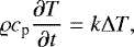
was solved for the temperature T throughout the whole domain (volume of the respective region as shown in Fig. 2), with adiabatic boundary conditions on the plane surfaces (i.e., no heat flow across the boundary). The physical parameters determining the thermal evolution are summarized in Table 2. The thermal inertia was chosen at the upper end of the expected range  . The thermal conductivity was determined through k = I2∕(ρcp), with the thermal inertia I, the density ρ, and the heat capacity cp chosen in accordance with the recent literature (Schloerb et al. 2015).
As mentioned in the introduction, the simulations presented in this paper do not consider sublimation of water ice from the surface or near-subsurface, similar to the preconditions of the study by Schloerb et al. (2015). This means that the temperature distributions obtained from our simulation are rather realistic for a dust-covered surface, but not for a surface or subsurface containing sublimating ice. To model sublimating parts, both the heat Eq. (1) and the surface boundary condition had to be adapted appropriately, as was done by Kömle et al. (2017) for simulations of the Abydos region of comet 67P. As another simplification, we assumed that all physical parameters describing the medium (Table 2) were constant, that is, that they do not depend on temperature, location, or time.
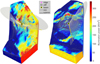 |
Fig. 2 Regions containing Spot 1 (left) and Spot 2 (right) in the COMSOL mesh as used for numerical simulations. The surface is colored according to solar irradiance at the respective MIRO observation time. The gray cones are the rays from the Sun to the spot centers during one cometary rotation; the yellow straight line refers to MIRO observation time. The black straight line points toward the spacecraft. Spot 1 is about 1 km long, and Spot 2 about 3 km (vertical extension in figure). |
4.2 Boundary conditions
On the uneven comet surface, a graybody boundary condition is usually applied, which means that the emissivity is independent of the frequency. We modified this assumption by applying a two-bands graybody boundary condition, which splits the whole frequency range into the band above 2.5 μm wavelength, where most of the thermal emission from the surface lies, and the band below 2.5 μm, representingthe main part of the solar irradiation. The former band is described by a constant microwave and infrared emissivity ε = 0.95 (Schloerb et al. 2015), and the latter by a constant optical albedo A = 0.062 (Ciarniello et al. 2015), which corresponds to a solar absorptivity (1 − A). These conditions are implemented in the COMSOL solver by defining a “Diffuse surface” boundary condition at the comet surface, with the parameters defined as given above and the option “Include surface to surface radiation” activated. This means that the surface emits thermal radiation isotropically, that is, the emitted radiance (power per unit solid angle per unit projected area) is independentof the direction, and the surface reflects incident radiation isotropically, that is, according to Lambert’s law.
On the boundaries of the simulation domain that are not part of the comet surface (the bottom and the sides of the domain), adiabatic boundary conditions were applied. Although these conditions do not represent the real situation exactly, they do not impair the solution in the area of interest (the respective spot). The reason is that on the one hand, the typical heat flux crossing these boundaries is far lower than the heat flux at the comet surface, and on the other hand, the simulation time interval is too short for a perturbation of the conditions at these bottom and side boundaries to reach the spot area (under the assumption of the same initial condition).
4.3 External radiation source
To represent the solar irradiation, a so-called external radiation source with a temperature of 5780 K and a power of 3.846× 1026 W was defined,where the time-dependent position of the Sun (considered here as a radiation point source) is given as
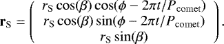 (2)
(2)
Here Pcomet = 12.404 h is the cometary rotation period (Preusker et al. 2015), β and ϕ are latitude and longitude of the Sun in the comet-fixed reference frame (CFF), and rS is the distance of the comet from the Sun (Table 1 lists the values of β, ϕ, and rS at the MIRO observation times of Spots 1 and 2).
Values of the physical parameters used in the 3D thermal model.
4.4 Initial conditions
The next step in setting up the simulation in COMSOL was to define the initial temperature distribution within the whole domain. Forthis purpose, we exported the simulation mesh from COMSOL and calculated the initial temperatures at the mesh nodes, which were imported back into COMSOL and used to define an interpolation function representing the initial temperature throughout the volume. The initial temperature calculations were performed in MATLAB on the basis of a 1D COMSOL model, assuming that the initial temperature at an arbitrary node of the volume mesh only depends on the distance from the comet surface (the distance from the nearest surface node). This procedure yields sufficiently accurate temperature estimates because the 3D simulation was run over eight comet rotations prior to the respective MIRO measurement time (small modifications of the initialtemperatures within reasonable bounds do not change the results at the last rotation).
The initial 1D temperature-depth model was obtained by a 1D simulation over ten orbital periods of the comet around the Sun. A similar long-time simulation for the fully 3D model is not feasible because of the long computation time. The 1D simulation was performed for several typical surface orientations occurring in the respective region, and the results were averaged to obtain a function Tini (d), where d is depth below the surface, as shown in Fig. 3. The 1D results for various surface orientations differ mostly in the uppermost decimeter. There, moderate deviations play no substantial role for the 3D simulation results: after several cometary rotations, a quasi-stationary periodic evolution has established that mainly depends on the solar illumination, the boundary conditions, and the initial large-scale dependence of Tini on d (decimeters to meters).
Becausewe have no information on the temperatures at depths of meters to kilometers, and because the near-subsurface temperatureat the beginning of the ten orbits plays no role for the result at the end, we assumed a constant temperature of Ti = 30 K throughout the whole nucleus (the whole 1D simulation domain) at the beginning of the ten orbits. In order to check the effect of Ti on the simulation results, we repeated the whole procedure (1D simulation to find Tini (d) from Ti with subsequent 3D simulation based on Tini(d)) for Spot 1 with Ti = 50 K. This study of the effect of Ti on the final simulation result is discussed in Appendix B, showing that even an increase of Ti by 20 K cannot essentially affect the outcome of our investigation.
The mentioned Ti values were chosen in such a way that they set plausible limits for the temperature in the deep interior (most of the volume) of the comet nucleus, where a value close to the lower bound of 30 K is favored for the following reasons: (1) the evaluation of the N2 ∕CO measurements of the Rosetta Orbiter Spectrometer for Ion and Neutral Analysis (ROSINA) led Rubin et al. (2015) to the conclusion that the cometary grains formed at temperature conditions below 30 K. (2) From geomorphological investigations, Groussin et al. (2015b) inferred a gentle formation process by accretion at low velocities of 1 m s−1 or lower, and that the nucleus did not undergo global melting or freezing of its water content (excluding radiogenic heating during the accretion stage as well as later exothermic phase transition of water ice from amorphous to crystalline condition). (3) The most important cause of a potential temperature increase above 30 K therefore is surface heating by insolation and subsequent conductive heat transfer from the surface to the interior. However, Skorov et al. (2016) showed thatice sublimation in near-surface regions does not only cause substantial surface ablation, but also prevents an appreciable temperature increase below a depth of about 10 m. Thus, the active comet does not come to a thermal equilibrium and the center temperature stays close to the formation value. The exact knowledge of Ti is not a precondition for our analysis in any case, as expounded in Appendix B.
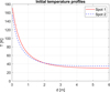 |
Fig. 3 Initialtemperature profiles based on a 1D model calculation for Spots 1 and 2. |
4.5 Mesh construction
Special attention must be devoted to establishing a suitable 3D simulation mesh throughout the whole volume. The cometary near-surface material is very porous and composed of micrometer- to millimeter-sized grains (Thomas et al. 2015), which implies a low bulk density and a very low thermal conductivity. This means that steep thermal gradients develop within a few centimeters below the surface. On the other hand, the typical beam width of the MIRO antenna on the cometary surface was on the order of several hundred meters (Table 1). These two conditions demand extremely high numerical resolution in vertical direction (from the surface into the cometary interior), but allow a much coarser resolution along the surface. To meet this requirement, a volume grid must be constructed in the near-surface layer with a vertical resolution in the millimeter range, whereas the lateral extension of the numerical cells must be orders of magnitude larger to restrict the total number of mesh elements to a manageable amount (with regard to computation time as well as computer memory). These conditions can be fulfilled using a suitable boundary mesh consisting of thin prisms near the cometary surface of the computational domain. The prism mesh starts with 0.3 mm thick prisms at the surface, becoming coarser with depth, and at about 2.5 m depth, the mesh turns into a tetrahedral mesh that extends below 2.5 m over the rest of the volume, with tetrahedra edge lengths of at least about 10 m. Figure 2 shows the surface of the final simulation mesh for Regions 1 and 2; faint lines indicate the edges of the mesh facets on the surface.
5 Results of 3D simulation: near-surface temperature field
In this section the results of the 3D simulations are discussed in terms of the evolution of the temperature distribution in the uppermost subsurface depth region of some decimeters. We focus on the surface temperature in Sect. 5.1 and on the temperature distribution in subsurface layers in Sects. 5.2 and 5.3. The temperature gradients are studied in Sect. 5.4.
5.1 Temperature distribution on the cometary surface
The two MIRO measurements that we chose to investigate were taken after sunrise at the observed spots (about 1.5 h at Spot 1 and 15 min at Spot 2), as can be recognized from Fig. 2. This means that the temperature on the surface of the target regions rose further after the respective measurement. The temperature distribution on the surface of Regions 1 and 2 at the measurement time t0 and one- to three-quarter comet rotations (multiples of 3.1 h) afterward are depicted in Fig. 4. The surface temperatures undergo a huge variation over one full rotation period, decreasing below 100 K at night and rising to about 300 K during daytime.
The irradiation maps in Fig. 2 show that at the time of the respective MIRO measurement, the illumination was stronger on Spot 1 than on Spot 2. Higher temperatures are therefore expected around Spot 1 at measurement time, which is confirmedby the simulation results. By means of the uppermost plots in Fig. 4, we can guess an average surface temperature at Spots 1 and 2 (compare also Fig. 2 to check the 2 FWHM area) at t = t0 of about 200–210 K and 130–140 K, respectively. A comparison with MIRO measurements is given in Sect. 8.
5.2 Temperature evolution in the subsurface region
Three types of plots were made to visualize the underground temperature: straight line cuts, plane vertical cuts, and plots for a given depth below the comet surface. These cuts were made at three different points in each region, marked by stars in Fig. 2: one point on a ridge, one at the foot of a cliff, and one in the spot center (MIRO beam center intersection with the comet surface). For Spot 1, all three points lie within the 2 FWHM beam cone of the MM channel, while for Region 2, the ridge and the cliff points lie outside the spot area. Figure 5 zooms on part of the spots so that these points and their surrounding facets are clearly visible. The beam center point is inside a mesh facet, whereas the ridge and cliff points are chosen on nodes where several facets meet. Figure 5 shows that the number of facets with a common node point varies from point to point: for Region 1, the ridge node is surrounded by five facets, the cliff node by seven facets, and the beam node by six facets; Region 2 has seven facets for the ridge point, five facets for the cliff point, and six facets for the beam point.
Because no unique surface normal is associated with surface nodes, we introduce the “sight depth” d′ as independentvariable, that is, the distance from the surface along a straight line connecting the position of the spacecraft (the center of the MIRO antenna) with the position of the respective point at the comet surface. We note that d′ is different from the normal depth d below a facet, which means the minimum distance of the respective underground point from the plane containing the facet. For near-surface points below a facet, d′ is related to d by
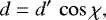 (3)
(3)
where the line of sight encloses an angle χ with the facet surface normal.
Figure 6 illustrates the temperature T(t, d′) as a function of time and sight depth for the center of Spot 1. The shown time interval corresponds to one cometary rotation, beginning atthe time of the MIRO measurement. This is the eighth rotation period in the numerical simulation. A comparison of the T values at the beginning and end of the interval proves that the simulations came to an almost periodic evolution. Only a very tiny increase of the temperatures can be found (scarcely visible in the plots). This is an expected effect because all our investigations treat inbound times when the comet was approaching the Sun, and the slight change of its solar distance over the eight simulated rotation cycles is not taken into account in our simulation. It is instead assumed that the comet had a constant distance from the Sun over the whole simulation time. The plots in Fig. 6 show how the heat absorbed from solar irradiation is slowly transferred to lower layers. The illumination of the spot center starts about 1.5 h before the time of measurement and ends almost 5 h afterward. Surface temperatures rise to 270 K after the Sun has passed its highest elevation and slowly decrease in the night, reaching about 120 K before the next sunrise. At 10 cm depth, diurnal variations are almost completely damped out and are hardly recognizable any longer in the plot. This is consistent with the low thermal conductivity used for the simulation, which results in a thermal skin depth
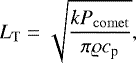 (4)
(4)
of only 1.5 cm. After solar culmination, a T-maximum develops below the surface that gradually drifts downward, passing 5–6 cm depth when MIRO scans Spot 1. When T starts to rise again on the surface, a T minimum also appears below the surface, above the maximum.
5.3 Temperature below observed spots
In principle,the evolution shows similar features below most surface points. In order to obtain an impression of the T distribution in subsurface layers over a larger area like the whole spot (2 FWHM of the MM channel), we plot the temperature functions T(Ω) at several fixed sight depths d′, where Ω denotes the direction at which subsurface points are seen from the spacecraft. The result is depicted in Fig. 7 for six sight-depthsd′ down to a maximum of half a meter. The selected points are again shown as stars, with the same colors as in previous figures (the ridge and cliff point are outside the plot for Spot 2). The T distribution on the surface is subject to large variations, which are damped out when deeper layers are reached. For instance, at the surface of Spot 1, the temperatures reach far higher values, but also decrease more strongly during night time than at a depth of d′ = 5 cm. This is an effect of the energy balance between incoming illumination and thermal emission from the surface.
Although the T variation decreases with depth because of the balancing heat conduction in the subsurface volume, the main features at the surface remain perceptible even at 50 cm depth, although the average T drops by about 150 K. We plotted the T(Ω) distribution for many depths d′ below 10 cmdown to 1.4 m. Only the 50 cm result is shown in Fig. 7 because the structure of T(Ω) remains roughly the same in this depth range; the mean temperature decreases with depth. Comparing the layer plots for Spot 1 with those for Spot 2, we find that the temperature on the surface is higher for Spot 1, whereas the local maximum of T(d′) at about 5 cm depth, which is the consequence of the heat supplied to the spot in the previous illumination period, is slightly more pronounced for Spot 2.
Finally, it is of interest to compare the T plots for given depths with the radiant exposure per rotation, that is, the irradiation occurring during one cometary rotation. Figure 8 exhibits the radiant energy E(Ω) per unit area incident on the two spots. It is calculated by integrating the total surface irradiance (solar plus indirect radiation incident per unit area) over a full rotation period. Down to about d′ = 2 cm, there is no clear correlation between T(Ω) and E(Ω), which is very plausible because of the strong variation of the irradiation with time. However, at about d′ = 5 cm, the high exposure features in E(Ω) are also perceptible in T(Ω). This correlation is weak because the temperature variation at d′ = 5 cm is very small and so the neighboring layers with different temperature distributions have a “smearing” influence on T(Ω). The situation is again different below about d′ = 10 cm: the plot for d′ = 50 cm exhibits a weak anticorrelation between E(Ω) and T(Ω) for the most part. This confirms that the temperature evolution in near-subsurface layers of fixed d′ is not only determined by the recent irradiation history, but also by the surface topology.
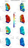 |
Fig. 4 Snapshots of the surface temperature distribution at the times t0 of the MIROmeasurement and multiples of 3.1 h (90° comet rotation) afterward. Coordinates of the CFF are given in kilometers. |
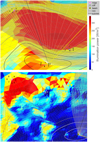 |
Fig. 5 Zooms into the surface areas of Spots 1 (top) and 2 (bottom), showing three selected points that lie on a ridge, at the foot of a cliff, and at the beam center. The facets surrounding the points are numbered, and cut lines through the points are drawn (magenta). The black straight lines point toward the spacecraft, and the yellow lines point to the Sun. The width of the area (left to right lower corner) is about 100 m in the top and 350 m in the bottom panel. |
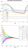 |
Fig. 6 Temperature T below the center of Spot 1 as a function of time t and sight depth d′. Here t = 0 is the time when MIRO scanned Spot 1. |
5.4 Temperature gradients and lateral heat flow
Owing to the non-monotonic nature of the function T(d′), there are, dependent on the solar illumination phase, subsurface layers with downward as well as upward heat flow. These layers can be well recognized from the T gradient plots in Fig. 9, which zoom on cross sections of the uppermost subsurface region of 0.8 m depth. The cross sections are obtained by an intersection of the subsurface volume with a plane containing the selected point (ridge, cliff), the MIRO sight line, and the center of one of the facets surrounding the selected point. The top panels show the resulting sections as they lie in the 3D reference frame (CFF). Figure 5 shows where these sections emerge on the surface (magenta lines through selected points). The left panels in Fig. 9 show the situation below the ridge point at the measurement time, and the right panels plot the situation below the cliff point before sunset when the heat flow changes from downward to upward. This choice enables us to discuss the size and properties of the lateral heat flow for two points in different surface topology (convex and concave) and for two different scenarios (measurement time and sunset with passing shadow).
The upper panels show the respective cross sections color-coded according to the temperature distribution. In the top right panel the normal and tangential unit vectors, n and t, which are associated with the two facets, are added at the selected cliff node. An analogous definition holds for the ridge facets. The gray (black) vectors are used to represent the normal and tangential components n ⋅∇T and t ⋅ ∇T of the temperature gradient below the left (right) facet. The position r below the surface is represented by
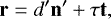 (5)
(5)
with n′ being the unit vector pointing from the spacecraft toward the surface point (we note that n′ ≠ n), d′ giving the sight-depth and τ the tangential distance along the facet surface. The representation is made unique by assuming τ ≥ 0 for the right facet and τ < 0 for the left facet. Because the definition of n and t change when passing the node (τ = 0) at a fixed sight-depth d′, the normal and tangential component of the T gradient, n ⋅∇T and t ⋅ ∇T, undergo a jump even when ∇T is continuous.
This effect can be recognized in the middle and bottom panels of Fig. 9, which depict n ⋅ ∇T and |t ⋅ ∇T| in the subsurface layer below the facets. Because considerable T variations occur only in the shown uppermost decimeter, we chose a log (d′) scale for the sight-depth (ordinates) but a linear scale for the tangential distance (abscissae) from the reference point (ridge or cliff node). At the ridge, positive abscissa values run across facet 3 and negative values run across the opposite facet 5. At the cliff, positive values refer to facet 1 and negative values to the opposite facet 4.
The normal fraction of ∇T dominates in most of the volume. In the middle panels the yellow to red part of the color scale corresponds to downward heat flow, pink to violet to upward heat flow. The tangential part is greatest close to the node (reference point, abscissa origin), which can be explained by the fact that an angle is formed between the opposite facets through which the plotted section cuts. The tangential component may only grow to some percent in the close vicinity of the node, otherwise, it is typically 0.1% of the normal component or less.
During periods of slow irradiation change, the isotherms in the top panels are almost equal to the lines obtained by shifting the surface by a multiple of the mean normal (average of unit normal vectors of the respective two facets). Because the angles χ in Eq. (3) for two non-parallel facets are different, the same isotherms as well as the lines of constant n ⋅ ∇T appear at different d′ values for τ < 0 and τ > 0, as can be seen in the middle panels of Fig. 9. Directly below the respective node, the tangent of the isotherms changes considerablywhen we pass below the node at a fixed depth. Because the change is not discontinuous, it happens gradually within a small interval τ ∈ (−ɛ, ɛ). There t ⋅∇T has a pronounced peak because the isotherms are not exactly parallel to the lines obtained by shifting the facets parallel to the sight-view n′.
As the solar irradiation decreases, a layer of upward heat flow appears below the surface. For the facets surrounding a node, this happens at different times if they have different orientations with regard to the solar rays. In the right panels, such a time is chosen to illustrate its effect on the subsurface T distribution.In this special case, the tangential flows are relevant around the border between the down- and upflow regions, building a sort of terminator between down- and upflow. It wanders over the surface (the uppermost subsurface layer of some millimeter depth) following the Sun, passing surface points in advance of the actual day-night terminator, for example, by about 1 h for the ridge point and beam center, 20 min for the cliff point (Spot 1). We find thus that a significant lateral heat flow (tangential temperature gradients) appears only close to acute surface corners and hypersurfaces that separate upflow and downflow subsurface regions.
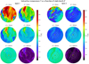 |
Fig. 7 Subsurface temperature distribution at different depths d′ (along the MIRO line of sight) at the respective MIRO observation time. Stars show the same selected surface points as in Fig. 2, and circles refer to 1 FWHM and 2 FWHM beam widths of the SubMM and MM channel. The horizontal axes of these plots are aligned with those of the respective spots in Fig. 2. |
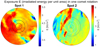 |
Fig. 8 Radiant exposure E per cometary rotation across the spots. E is obtained by integration of the irradiance over one cometary rotation. The alignment of the axes in these plots is the same as in Fig. 7. |
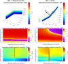 |
Fig. 9 Temperature and its gradient across plane cuts in Spot 1: through the ridge point at the measurement time (left), and through the cliff point before sunset, when the heat flow changes from downward to upward (right). The normal component of ∇T is positive for downward heat flow. |
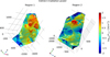 |
Fig. 10 Indirect irradiation in Regions 1 and 2 due to surface-to-surface radiation interaction. The surface is colored according to the logarithm to the base 10 of the indirect illumination power Pind. |
6 Indirect facet irradiation
In the framework of our simulation, the total radiation power supplied to the cometary surface comes from the Sun. However, an individual facet receives not only the direct solar irradiation, but also indirect radiation from other facets, leading to self-heating of the comet. This indirect (mutual) part is a consequence of the thermal emissions from other parts of the surface that are within the FoV of a particular surface facet. The dominant part of these emissions lies in the microwave and infrared range.
It is instructive to compare the direct external irradiation from the Sun exhibited in Fig. 2 with the indirect radiation share that causes self-heating of the surface. Figure 10 shows the indirect irradiance, that is, the power per unit area Pind that is incident to the surface coming from thermal emissions of the surrounding surface. The common logarithm, log10(Pind∕(W m−2)), is plotted to emphasize the weaker part of the scale because it dominates the surface. Only in concave areas is the indirect radiation significant; in pronounced (rare) cases, it becomes as strong as 100 W m−2. Nevertheless, this is not the typical situation. The average re-radiated flux absorbed at other regions is some W m−2, which is on the order of 1% of the direct solar illumination.
Therefore we can expect that indirect radiation has some influence at points where the terrain is particularly rough and shadows cover a great portion of the surface. This means that strongly illuminated facets that cover a great solid angle when observed from an opposite shadowed facet would provide considerable indirect radiation to the latter. No such situation occurs for the selected ridge points, but it may well occur for the cliff points. In order to verify this in more detail, the indirect (mutual surface-to-surface) irradiance Pind was compared with the total irradiance Ptot = Pind + Pext, where Pext is the direct solar irradiance (called “external” in COMSOL). The ambient background radiation can be neglected. The time-dependence of Pind and Ptot in the centers of some facets surrounding the nodes selected above is depicted in Fig. 11 for a full cometary rotation.
Pind lies below about 10 W m−2 for the ridge and beam curves. Nevertheless, the illumination around a ridge node may vary significantly from facet to facet, with up to about 25 K maximum T offsets and about an hour phase-shift for the investigated points. As expected from the discussion above, the cliff points exhibit a stronger influence of the indirect irradiation. In general, this effect is stronger for Region 2 than for Region 1. This is plausible because at the respective measurement time, the Sun had a lower elevation over the horizon at Region 2, so that a larger portion of the facets was shadowed. In particular, the cliff point in Region 2 was chosen in a dent (almost an overhang), therefore it is expected that it exhibits the greatest difference between Pext and Ptot of the points we studied. It is the only point where the indirect radiation is so strong that it plays a dominant role. One facet (F2) surrounding this cliff point is even in permanent shadow and sees no Sun over the whole rotation period.
In summary, the effect of indirect radiation is strongest where the direct illumination is missing (cavities) or where it suffers abrupt spatial discontinuities (in the vicinity of shadows or terminator). The effect of indirect radiation on the tangential heat flow is complicated because it crucially depends on the topology. The effect may be negligible when the mutual radiation comes from a wide area, but it can be significant where facets enclosing an acute angle are illuminated by indirect radiation from a close opposite area that is seen by only one of the neighboring facets. This consideration confirms that uneven terrain and surface roughness have a significant influence on the heat balance of the comet.
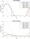 |
Fig. 11 Total surface irradiation (top) compared with indirect solar irradiation (bottom) in the center of facets at selected points in Regions 1 and 2, where the temperature evolution is studied in detail. |
7 1D heat transfer model and comparison with 3D simulations
The considerable variation of facet orientations may cause entirely different solar irradiation histories and cause large variations in the corresponding T(d) profiles, even within regions that are very small compared to the comet size. For example, this is the case for facets sharing the same mesh node as corner when the facets are tilted with regard to each other. The different T profiles in the subsurface under neighboring surface facets cause lateral T gradients (T variation along the facets) and tangential heat flows. For the measurement times, we found typical lateral T gradients of some K m−1, but they may vary by an order of magnitude, being smaller in large flat regions and greater near acute angles. Most facet edge sizes in our 3D simulations range from 10 to 50 m, so that we can expect typical T-differences of 10–50 K between adjacent facet centers (if the facets do not lie in shadows). In rare cases with acute angles between neighboring facets, thesevalues may be exceeded. Such high temperature differences occur both for convex (ridge) and concave (cliff) areas and may appear in any local daytime, but they are most conspicuous when the main heat flow orientation changes from downward to upward or vice versa (Fig. 9, right panels).
Because no tangential T gradient is taken into account in 1D heat transfer models, a comparison of the temperature evolution obtained by 1D and 3D simulations can indicate whether tangential heat flow plays a significant role for the heat balance in subsurface cometary layers. For this purpose, we made 1D simulations on the basis of the following model: the centers of the facets around the selected ridge, cliff, or beam points were used as a reference, using their respective irradiation (including indirect irradiation) history obtained by the 3D simulation as boundary condition. The solution of the 1D heat transfer equation was calculated under this boundary condition on the surface and an adiabatic boundary condition at the interior end of the computational domain (meters apart). The results of these calculations give the temperature evolution on straight lines normal to the surface.
A comparison of 3D and 1D results is depicted in Fig. 12 for center points of the selected facets. The solid lines refer to 3D and the dashed lines to 1D. The figure shows the scenes at sunrise, sunset, and the measurement time for the selected facets. The temperature T is shown as a function of depth d along the respective facet normal. The temperature on the surface was usually lowest at sunrise (blue curves), increased until the time when MIRO scanned the facet (green curves), and reached maximum before it decreased to the value shown for sunset (red). The temperature evolution below the points in Region 2 is different from the respective points in Region 1 because the points lie at the different positions and the facets are oriented differently with regard to the incident sunlight.
Although the typical tangential heat flow was only about 0.1% or less of the normal heat flow (Fig. 9), the resulting difference between 3D and 1D temperature may increase to about 30 K within short periods of time. Particular reasons are discussed in the following. In general, the largest deviations occur at surface points when part of their neighborhood is much lessilluminated than the rest. This may be caused by a passing shadow or terminator or by a sharp edge between neighboring facets. The latter situation occurs, for instance, around the ridge point of facet 4 in Region 2.
As expected, we find that of all types of points, the ridges gain most temperature from sunrise until t0 because of their exposed position. Sharp edges at peaks or ridges may be responsible for considerable lateral heat flow. In contrast to this, there may be areas in depressions that are not insolated at all, for instance, places that are surrounded by wide cliffs, such as the cliff facet 2 in Region 2. Nevertheless, such places may heat up between sunrise and measurement time through indirect radiation. For example, at the center of cliff facet 2 in Region 2, T at t0 has increased byabout 50 K over its value before sunrise because it receives strong indirect radiation from the whole surrounding cliff (red area in the right panel of Fig. 10), which is illuminated earlier than the spot center. Here indirect radiation by diffuse reflection from the surrounding may reduce the dependence on the exact position and facet orientation, and it causes less tangential heat flow, explaining the negligible deviation between 3D and 1D in the example described above.
In the middle of flat areas that are distant from elevations, the illumination is relatively constant over most of the daytime, so again the deviation between 1D and 3D is small, and is only significant for a short time after sunrise and around sunset. For example, this situation prevails in the beam centers, as illustrated for beam facet 4 in Region 1 in Fig. 13. It represents the typical behavior in a good portion of the spot. The top panel depicts the evolution of the temperature profile, T(d, t), as found by 3D simulations, the bottom panel gives the corresponding difference between the temperatures obtained by 1D and 3D simulations. The slow downward drift of surface T perturbations is clearly visible; they become weaker with depth. A comparison of Figs. 12 and 13 shows another interesting effect. The differences in 1D and 3D T reach about a decimeter below the surface, where they become negligible (far below 1 K). At the surface, they are most pronounced after sunrise and before sunset, the features of the T evolution reaching about 5 cm depth half a cometary rotation later. The deviations between 1D and 3D are largest near local maxima and minima of the T(d) functions for fixed t, the 1D simulations amplifying the extremes. This finding verifies that the differences are due to the omission of the tangential heat flow in the 1D model. The tangential heat flow counteracts high temperature gradients on the surface and at subsurface levels, so that it has a balancing effect that mitigates temperature extremes and reduces normal heat flow.
Becausethe MM-wave penetration depth (according to Schloerb et al. 2015 about 4 cm) is sufficient to see the subsurface layer where differences between 1D and 3D are significant, the MM observations may, in principle, be influenced by lateral (tangential) heat flow. However, we have to emphasize that this is not the case for our simulations. The reason is that they are based on a surface mesh that is smooth for the wavelengths received by MIRO. However, we should not disregard that the real surface of the nucleus is rough and ragged, with a potentially stratified subsurface structure. This complex surface is strewn with grains, boulders, and fissures, and so with as many shadows that permanently move with daylight. Applying our findings to this situation, we therefore would expect a perceptible influence on the MM measurements.
This assessment is of even greater importance when materials with different thermal properties lie side by side or one on top of the other.A layer of low conductivity would block thermal heat flow, giving even more weight to tangential heat flow, which may considerably depend on the presence of such layers. The effects we described above may explain at least part of the difference between the MIRO observations and our theoretical results for the MM channel discussed below.
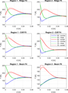 |
Fig. 12 Comparison of 3D with 1D simulation results for the temperature-depth profile T(d) below the centers of 3 selected facets in each region, at the respective sunrise, sunset and measurement time. |
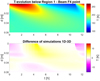 |
Fig. 13 Evolution of the temperature profile T3D obtained by 3D simulations (top) and the corresponding difference T1D − T3D between 1D and 3D simulations (bottom). Abscissas and ordinates represent time after MIRO measurement and depth normal to surface, respectively. |
8 Comparison with MIRO measurements
8.1 Calculation of antenna temperature
The 3D simulation results are now used to “predict” the brightness temperatures TB that MIRO is expected to measure when observing either of the two spots. For this purpose, we calculate the antenna temperatures TA, making the following simplifying assumptions: the microwave radiation seen by the MIRO antennas stems from emissions on the cometary surface and a subsurface layer with a sight-depth of at most smax = 1.5 m. The microwaves received by the MM and the SubMM channel have a subsurface penetration depth (attenuation length) of about LA = 3.9 cm and LA = 1 cm, respectively (Schloerb et al. 2015). The antenna gain can be represented with sufficient accuracy by the formulas given by Frerking et al. (2018). The resulting antenna gain pattern based on these assumptions is shown in Fig. 14 for both channels. Each function is Gaussian around the main lobe (falling to half its maximum at the angle θh = FWHM∕2) and gives a suitable fit of the gain outside, with the side lobes being levelled off.
Because Frerking et al. (2018) gave the normalized gain, we had to determine a multiplication factor (the maximum gain Gmax in the direction of the symmetry axis) in such a way that ∫ G(Ω) dΩ = 4πη, where η is the antenna efficiency (which we assumed to be 1). We obtain Gmax = 2.45 × 10⁵ for the MM and Gmax = 2.28 × 10⁶ for the SubMM channel.
With these assumptions, the antenna temperature TA, which is a measure of the received power, can be calculated on the basis of Eq. (A.5) as briefly explained in Appendix A. The integral in Eq. (A.5) can be regarded as the convolution of the antenna gain with the brightness function of the observed target in the respective frequency channel, taken at the current antenna direction. It has to be extended over the part of the volume seen by the antenna. We found that emissions beyond the 2 FWHM cone may contribute to TA in the MM channel (about 15 K for Spot 1 and 12 K for Spot 2), whereas contributions outside the 3 FWHM cone (θ > 3θh) are negligible. In accordance with the gain pattern beyond 2 FWHM (Frerking et al. 2018), this was to be expected because there are no extraordinary differences between the mean T inside and beyond 2 FWHM. We therefore decided in favor of the 3 FWHM integration domain, which resulted in the values given in Table 3. In addition to the antenna temperatures TA, the brightness temperatures TB were calculated by means of Eq. (A.8). This means that a blackbody at constant temperature TB filling the whole solid angle seen by the antenna (e.g., 3 FWHM or more) would generate the same antenna temperature TA.
The following procedure was applied to perform the numerical integration. The temperature field across the volume inside the 3 FWHM cone, from the cometary surface down to the depth smax, was exported from COMSOL. From this, a volume grid was created that was very dense close to the surface and close to the beam center2 ; the spacing of grid points (Fig. 15) became wider with depth and with distance from the beam axis. The exported data were read into MATLAB where the integration is performed, applying linear interpolation of T between the exported points.
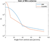 |
Fig. 14 Gain of the MIRO antenna for the center frequencies of its two channels, calculated according to Frerking et al. (2018), as a function of the angle θ from the symmetry axis. |
Antenna temperatures TA and associated effective brightness temperatures TB obtained on the basis of finite-element simulations, compared with corresponding MIRO measurements.
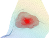 |
Fig. 15 Grid of points (red) for the temperature export from COMSOL for the numerical TA integration. |
8.2 Simulation results
Table 3 reveals that the simulation results are in good agreement with the measurements for the SubMM channel. The SubMM brightness temperatures lie slightly below the average surface temperatures for Spots 1 and 2 of about 200–210 K and 130–140K, as estimated in Sect. 5.1. This was to be expected because on the one hand, the emissivity is lower than 100%, and on the other hand, the subsurface regions at lower temperatures contribute to the integral in Eq. (A.5).
In contrast to the SubMM channel, the MM channel shows significant discrepancies (18 K for Spot 1 and 12 K for Spot 2) between calculations and measurements. The different degrees of agreement in the SubMM and MM channels are independent of the use of a 3D or 1D model. Hence some of the assumptions in our thermal emission and/or antenna reception model may be inadequate. In the following, potential reasons are listed, which are worth being considered in future studies:
- 1.
the gain model is not exact because side lobes are not taken into account at all. If MM side lobes were to occur at regions with very high temperatures, the simulation results would be shifted toward the measured values. However, the gain of side lobes is 30 dB or more below that of the main lobe, therefore we cannot expect corrections of much more than 1 K. To determine the influence of a slight misrepresentation of the gain, we modified the MM FWHM by 2 arcmin but only obtained a change in TA of about 0.3 K.
- 2.
We did not consider the effect of spillover losses occurring in the MIRO optical bench. They may be responsible for a contribution of the sky above the spacecraft to the measured TA. According to Frerking et al. (2018), this effect would be similar for both channels, which means that spillover cannot explain the extremely different reproducibility of the MM and SubMM observations.
- 3.
The indirect illumination (facet-facet radiation interaction) is taken into account in the temperaturesimulations, but the reflected microwaves have not been included in the calculation of TA. However, a rough estimate of their average contribution to TA yields only a value below 1 K. An exact treatment of all reflections (whole cometary surface and Sun) may lead to a higher contribution, in particular when the side lobes are taken into account.
- 4.
The assumed microwave penetration depths may be inaccurate. They depend on the material properties in the near-subsurface region. In particular, we did not account for a potential variation of thermal, mechanical, and dielectric properties in the near-subsurface, for example, a variable dust/ice ratio or sinter crusts. The assumption of a homogeneous medium is probably far from reality, particularly in the near-subsurface region (see also last item below). Because the propagation of the microwaves depends highly on the structure and the material properties of the medium, this could well be the reason for the large discrepancy between the MIRO TA measurements in the MM channel and our 3D simulation results. A reduction of LA = 3.9 cm would bring the simulation result for Spot 1 closer to the measurement because the lower subsurface temperatures contribute less. However, even an extremely low value of 1 cm is not sufficient to reach as high a value as the measured 175 K for Spot 1. Furthermore, this is no explanation of the physical effects that are responsible for the difference in the MM and SubMM reproducibility.
- 5
Internal reflections of subsurface microwaves at the cometary surface are not allowed for. The surface reflectivity depends on the dielectric constant ɛs of the subsurface material that also determines the penetration depth LA. A significant dependence of the surface reflectivity on the emission angle may also change the observed brightness. Because ɛs depends on frequency, the two channel frequencies may have slightly different surface reflectivity (also important for the indirect reflections).
- 6.
Another effect might make a decisive difference between the SubMM and MM frequencies: (sub)millimeter-sized sand/dust grains on the surface or other types of surface stratification. For instance, Thomas et al. (2015) showed that dust deposits due to material transport and airfall of non-escaping particles can significantly influence the appearance of the nucleus and so the surface thermal properties. The emissions may therefore become extremely frequency dependent in the micro- to millimeter wavelength range as a result of multiple reflections and scattering inside such a particle layer as well as scattering on the surface (effect of roughness).
- 7.
All our calculations are based on constant material parameters, which is of course an oversimplification. For instance, the temperaturedependence of the thermal conductivity can be responsible for a considerable change in average heat transfer toward the center, as shown by McKay et al. (1986) on the basis of a spherical nucleus. Any layering of comet material, not only very close to the surface, can therefore have a strong effect on the evolution of the T(d) subsurface profile.
- 8.
Finally, inadequate initial conditions could be responsible for the inaccurate calculations of the MM observation. In particular, we may assume that the initial 3D simulation temperatures Tini were too low for deep regions (e.g., below the uppermost decimeter). It is tempting to assume that this explains the too low MM TA simulation values, even though the simulation was quite stationary after ten cometary rotations. Therefore, we investigated this question in more detail, as described in Appendix B. We found that a 20 K increase in core temperature of the comet ten orbits ago would only have an effect of 1 and 0.4 K on the observed antenna temperature in the MM and SubMM channel, respectively.
A detailed study of items 1–7 is beyond the scope of this article. It is essential for the solution of the inverse problem, that is, to find the parameters determining the surface and subsurface properties (in particular, thermal inertia, thermal conductivity, and dielectric constant) from the measured antenna temperatures. Nevertheless, our results prove the importance of a suitable integration over the whole spot area as well as along the line of sight to a sufficiently deep subsurface level. In order to quantify this assessment, the antenna temperature was calculated for various penetration depths LA for both MIRO channels, and the results are listed in Table 4. We find that TA considerably depends on LA, monotonically decreasing with LA for Spot 1, and possessing a maximum at about 5 cm for Spot 2. The difference between Spots 1 and 2 is plausible in view of the subsurface T(d) maximum caused by the solar radiant energy input during the previous day. In the case of Spot 2, this maximum well survives until the measurement (about 15 min after sunrise), but for Spot 1 the maximum has almost vanished at the measurement (about 1.5 h after sunrise). Only the SubMM observation of Spot 2 is close to the surface average (LA = 0), the other measurements can only be explained by subsurface emissions. This confirms the great relevance of the integration over subsurface layers. Similarly, we can emphasize the relevance of the integration over the whole main lobe of the MIRO antenna by comparison with what would be measured if the whole spot were at the same temperature Tc as the spot center. With Tc = 246 K and Tc = 143 K from the 3D simulations for Regions 1 and 2, we obtain by means of Eq. (A.7) the following antenna temperatures: TA = 229 K (MM) and TA = 221 K (SubMM) for Spot 1, and TA = 132 K (MM) and TA = 123 K (SubMM) for Spot 2. Only the MM Spot 2 simulation and measurement are less than 10 K away from these estimates, the others lie far apart. This verifies the importance of integrating over the whole main lobe solid angle, which was to be expected given the surface T distribution in the top panels of Fig 4.
Antenna temperatures TA as a function of penetration depth LA for the two MIRO channels.
9 Conclusions
The heat balance on the surface of cometary nuclei has been studied intensively in the past decades. In calculations of the temperature evolution of the uppermost subsurface layers, it was assumed that the heat flow is normal to the surface. In order to examine the validity of this precondition and its consequences, we applied a full 3D thermal model of the subsurface volume below two regions around spots on comet 67P that were observed by the Rosetta/MIRO instrument. The study was performed for a homogeneous dry dust layer with physical parameters in accordance with former works by other authors (Table 2). For this purpose, the heat equation was solved over a simulation domain that was wide enough to represent the shadow-casting by the surroundings of the observed spots. Furthermore, the domain was so wide and deep that adiabatic boundary conditions at the sides and at the bottom of the selected domain were applicable without sacrificing the accuracy of the approach. The boundary condition on the surface included a indirect surface-to-surface radiation, which plays a role in scarcely illuminated regions.
We found extreme temperature variations over the surface of the observed spots and very swift reaction of the temperatures to changes in solar illumination, which is a consequence of the low thermal inertia of the surface material. As expected, the heat flow is predominantly normal, with typical lateral fractions (tangential to the surface) of 0.1% or less. Only beneath edges between non-parallel surface areas (kinks) may the tangential heat flow exceed 1% at a lateral distance of several centimeters from the edge. The lateral heat flows rise at times when shadows pass the surface point, which may cause local temperaturevariations of up to 100 K between the centers of neighboring facets (10–20 m typical edge length). The most surprising effect was found by a comparison with 1D simulations with exactly the same surface boundary conditions (the same total irradiance and the same physical properties of the medium): in spite of the tiny average lateral heat flow in the 3D model, temperature deviations between the 3D and 1D simulation typically reach 10–30 K beneath the surface in time periods of strong illumination changes (in particular, along shadow margins and at sunrise and sunset). These differences are most pronounced where the temperature as a function of depth T(d) has a maximum or minimum. The position of maximum difference moves downward together with the T(d) maximum or minimum, typically dropping below 1 K at about 5 cm depth.
From the temperature field obtained by the 3D simulations, we calculated the power the MIRO antenna should have received in terms of the antenna temperature TA and compared it with the real measurement. The theoretical values are in good agreement with the observations of the SubMM channel. In contrast, a significant discrepancy of about 18 K for Spot 1 and 12 K for Spot 2 was found in the MM channel. The reason may be an inaccurate description of the antenna reception properties or omitted physical effects on the cometary surface that modify the thermal emission. Our analysis favors the latter explanation, especially surface roughness or subsurface stratification due to layers of different materials, for instance, dust deposits. If such a layer blocks radiation from deeper regions and amplifies the contribution of the uppermost layer, MIRO would observe the temperatures very close to the surface. In order to estimate this effect, we calculated TA as a function of the penetration depth LA for both spots. We find that an agreement of the MM observations can be achieved for Spot 1 when the emissions come from a layer of less than 1 cm thickness. This seems unrealistic unless effects of multiple wave reflections or scattering play a role, which may be extremely frequency dependent in this frequency range. However, for Spot 2, the high TA observation is not reached even for LA = 0 (only emissions from the surface). Finally, we addressed the question whether lateral heat flow might change the MM observations, with a tentatively positive answer. Although in our calculations the time periods and the spatial regions with significant differences between 1D and 3D results were too small to make a difference in the MM TA values, our results also show that a sufficiently rough surface can turn the lateral heat flow into a significant effect: with asperities of micrometer to many meter sizes, the surface is strewn with many shadows that move with daylight. In consequence, the surface and subsurface temperature in certain areas down to some centimeters may be significantly affected by lateral heat flow. These considerations summarize the most important of the effects, which we listed as factors of influence on the MIRO observations. We indicated which deserve further investigation to accurately quantify their contribution to the high TA values for the MM channel.
As a general remark on finding physical parameters of the subsurface material from MIRO measurements, we emphasize that it representsa theoretically underdetermined problem because so many unknowns (thermal properties, surface roughness, stratification, in particular, the variation in dielectric and thermal properties with depth) may affect the observed emissions. Nevertheless, we obtained a good reproduction of the SubMM observations, and a discrepancy for the MM channel provided clues about potential oversimplifications of the applied model.
Acknowledgements
We are indebted to the instrument teams of the Rosetta Mission, in particular, the MIRO and the OSIRIS teams, who provided the basis for the evaluation results reported in this paper. Y.S. thanks the Deutsche Forschungsgemeinschaft (DFG) for support under grant SK 264/2-1. The authors are grateful to the anonymous referee for comments that improved the manuscript essentially.
Appendix A MIRO antenna temperature calculation
Here we provide the most important relations for the calculation of the MIRO observations from the temperature field at the cometary surface and subsurface. More details on the theoretical part of the antenna analysis can be found, for example, in Collin and Zucker (1969). The MIRO observation is described in terms of the antenna temperature TA, which is a measure of the spectral power P received by the antenna from a source that emits thermal radiation. It is defined as
 (A.1)
(A.1)
where kB = 1.3806 × 10⁻²³ J K−1 is the Boltzmann constant and Γ the reflection coefficient at the load or antenna terminals; Γ = 0 describes a perfectly matched antenna. The motivation for this definition is that TA approximates the temperature of a load connected to the receiving antenna in thermal equilibrium if the thermal radiation has its spectral maximum in the radio frequency (RF) range. In this case, the received spectral power is equal to the spectral power that the load resistor at temperature TR would provide to the antenna,
 (A.2)
(A.2)
where the approximation (Rayleigh–Jeans law) holds for the radio frequency range. Here λ is the wavelength. B0 denotes the blackbody brightness according to Plank’s radiation law, which is a function of frequency f and temperature T:
 (A.3)
(A.3)
with Plank’s constant h = 6.626 × 10⁻³⁴ Js and the speed of light cL = 299792 km s−1.
The total power delivered to the load (receiver) at the receiving antenna is composed of two parts: first, noise from the resistive part of the cables or antenna system if the antenna efficiency η is below 1, and second, the spectral power received from the cometary surface and uppermost subsurface layers, given as a convolution of the antenna gain (beam pattern) with the brightness over the observed region,
![Mathematical equation: \begin{equation*} P = (1-|\Gamma|^2) \left[ (1-\eta) \frac{B_0(f,T_0)\lambda^2}{2} + \frac{1}{2}\int A_{\mathrm{eff}}(\Omega)B(\Omega)\,\mathrm{d}\Omega\right] .\end{equation*}](/articles/aa/full_html/2019/10/aa34798-18/aa34798-18-eq10.png) (A.4)
(A.4)
T0 is the temperature of the cable or antenna system, Aeff(Ω) is the effective area of the antenna, and B(Ω) is the brightness (spectral radiance) of the comet surface as seen from the antenna in the direction Ω. The brightness is the power per unit frequency per unit solid angle per unit projected area emitted toward the antenna. The integral is to be taken over the area on the cometary surface seen by the antenna, that is, the area where Aeff (Ω) has a non-negligible contribution. After substitution of Eq. (A.1) and introduction of the antenna gain 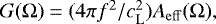 the antenna temperature becomes
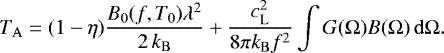 (A.5)
(A.5)
If the antenna is extremely efficient, the idealization η = 1 can be applied, which means that TA does not depend on T0 at all.
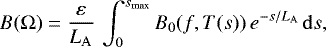
Becausethe surface material is not completely opaque at the frequencies of the MIRO channels, the brightness B(Ω) is composed ofcontributions from a subsurface region extending down to a depth of a few centimeters or decimeters. As a consequenceof the temperature variation with depth, the observed brightness depends on the penetration depth LA (we assumed a homogeneous subsurface material, implying a constant LA for each frequency; we also neglected that waves from the interior may suffer partial reflections at the surface; further discussion about simplifications is given in Sect. 8). Evaluation of MIRO data under the same assumptions by Schloerb et al. (2015) resulted in the following estimates for a homogeneous dry dust layer with a constant absorption coefficient: LA = 3.9 cm and LA = 1.0 cm for the MMand SubMM channel, respectively, and a thermal skin-depth of about 1 cm. The brightness B(Ω) can be calculated by integration along the line of sight (direction Ω) from the surface into the subsurface medium as
 (A.6)
(A.6)
with ε being the emissivity of the surface material (assuming a graybody model). B0 has to be evaluated as a function of the temperature T(s) at the depth s (sight-depth3) in the respective direction Ω. The integration is taken down to a sight-depth smax of many LA, so that there is no influence of regions beyond (still deeper layers). In our calculations we used smax ≈ 1.5 m.
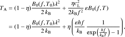
The Rayleigh–Jeans approximation (the right side of Eq. (A.2)) is usually applied to represent the brightness (spectral radiance) in the RF range. However, because the temperature may decrease to 50 K, the first-order Taylor expansion of the exp-term in Plank’s law is not sufficient, giving hf∕(kBT) ≈ 0.54 for the SubMM channel, which would result in significant errors in B0. Therefore we used Plank’s formula throughout. When an object of constant temperature T occupies the whole solid angle where the antenna gain is significant, the formula for the antenna temperature can be rewritten in the form
 (A.7)
(A.7)
which would further simplify to TA = (1 − η)T0 + ηεT in the RF range, and so TA = εT for highly efficient antennas (η = 1).
The antenna temperature data provided by the MIRO team take the influence of most noise sources we listed into account by means ofrecurrent calibrations, at least every 0.5 h and at every mode change (for details, see Frerking et al. 2018). Spillover effects in the MIRO optical bench are not taken into account here. In consequence, the delivered TA values are defined in a slightly different way, referring to the term in large parentheses in Eq. (A.7). In our terminology, this amounts to setting η = 1 in the application of the above formulas.
From the measured or simulated antenna temperatures TA, we calculate the effective brightness temperatureTB. It is the temperature of a (virtual) blackbody (ε = 1) that would generate the same TA value when the full solid angle were covered, where the gain is not negligible. This definition applies even if the temperature is not constant throughout the actually observed object or area. In general, (hf ≪ kBT is not necessarily fulfilled), TB is obtained by solving Eq. (A.7) for TB = T, giving
![Mathematical equation: \begin{equation*}T_{\mathrm{B}} = \frac{hf}{k_{\mathrm{B}}}\, \left[\ln\left(1+\frac{hf}{k_{\mathrm{B}} T_{\mathrm{A}}}\right)\right]^{-1} ,\end{equation*}](/articles/aa/full_html/2019/10/aa34798-18/aa34798-18-eq15.png) (A.8)
(A.8)
where we have set η = 1 for the reasons discussed above.
Appendix B Influence of initial conditions on 3D simulation results
The initial conditions of the 3D simulations are given by the temperature Tini throughout the simulation domain. We have represented it as a pure function of depth, that is, Tini (d) with d being the distance from the closest surface point. This function was determined for each spot by 1D simulations of the evolution of the T(d) profile for an average facet orientation over ten cometary orbits (roughly since the last encounter of 67P with Jupiter when its orbit changed to a perihelion below 1.3 au). It is assumed that the comet nucleus was at Ti = 30 K in the beginning. The result of the 1D calculations is the function Tini(d), which is used to create the initial conditions for the 3D simulations. The question arises how a change in constant Ti would change the 3D initial conditions Tini (d), and how it alters the diurnal T evolution and the MIRO antenna temperature TA.
To answer this question, we reran the 1D simulations over ten orbits for different values of Ti. The results for the last three orbits are plotted in Fig B.1 for Ti = 10 K (solid line), 20 K (dashed line), and 30 K (dash-dotted line). The upper and lower panels represent facets with normal vectors pointing to 60° northern and southern latitude, respectively.
As expected, we find that the temperature at 20 m depth is practically not affected by the heat exchange (insolation and thermal emission) at the surface during the past 60 yr. In a transition region between about 5 and 15 m depth, the temperature increases gradually without indication of orbital variation. The orbital variations are clearly visible at depths of about 1 m and less. Most important, we recognize that a modification of the temperature Ti by 20 K at the simulation start does not have any effect on the temperatures in a layer down to at least 25 cm below the surface. There the time dependence of the temperature has become periodic after the first few orbits, and no deviation from the periodic nature can be seen in the last three orbits. The evolution at the surface is shown as a gray curve, which looks like a gray band because of the strong diurnal variations.
From the results of the orbital 1D simulations, we find a rough upper bound of the temperature change ΔTini(d) after ten orbits (which serves as initial condition for the 3D simulations) caused by a temperature offset ΔTi :
![Mathematical equation: \begin{equation*}|\Delta T_{\mathrm{ini}}(d)| \leq |\Delta T_{\mathrm{i}}|\,\left[\frac{1}{20}+\left(1-e^{-d/L_{\mathrm{TO}}}\right)\right] ,\end{equation*}](/articles/aa/full_html/2019/10/aa34798-18/aa34798-18-eq16.png) (B.1)
(B.1)
where LTO is the thermal skin depth of about 1 m associated with the orbital motion.
This formula was applied with ΔTi = 20 K to calculate modified initial conditions Tini + ΔTini for another 3D simulation run (again eight cometary rotations). The results of these modified simulations are compared with the original results for the initial condition Tini. The difference between the final temperature fields in the observed Spot 1 is as follows: At the surface, fewer than 1% of the mesh nodes have a temperature increase ΔT of 1 K or more, and fewer that 0.1% are over 2 K, with a maximum ΔTmax ≈ 3 K and an average  . At 5 cm depth we find that ΔT > 1 K for 93% and ΔT > 2 K for fewer than 0.2% of the nodes, with a maximum ΔTmax ≈ 2.2 K and an average
  .
.
On the basis of the modified version of the initial temperatures, the MIRO antenna temperatures TA are calculated for Spot 1, giving 157.7 and 170.9 K for the MM and SubMM channel, respectively. We find that an increase in temperature of the cometary nucleus by about 20 K at a time about 60 yr ago results in a final increase of the calculated MM and SubMM TA values of 1 and 0.4 K, respectively. This proves that a shift of the initial temperature within the estimated bounds cannot explain the discrepancy between the accuracy of the SubMM and inaccuracy of the MM predictions.
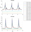 |
Fig. B.1 Subsurface temperature evolution on comet 67P for the last three orbits of a ten-orbits 1D simulation. The curves belong to different initial temperatures Ti and depths d. The results for two facet orientations are shown, corresponding to positions at 60° north (top) and 60° south (bottom) on a sphere. |
References
- Barbin, Y., Kofman, W., Nielsen, E., et al. 1999, Adv. Space Res., 24, 1115 [NASA ADS] [CrossRef] [Google Scholar]
- Choukroun, M., Keihm, S., Schloerb, F. P., et al. 2015, A&A, 583, A28 [NASA ADS] [CrossRef] [EDP Sciences] [Google Scholar]
- Ciarniello, M., Cappacioni, F., Filacchione, G., et al. 2015, A&A, 583, A31 [NASA ADS] [CrossRef] [EDP Sciences] [Google Scholar]
- Collin, R. E., & Zucker, F. J. 1969, Antenna Theory, 2 parts, Inter-University Electronics Series (New York: McGraw-Hill), 7 [Google Scholar]
- Coradini, A., Capaccionia, F., Drossart, P., et al. 1999, Adv. Space Res., 24, 1095 [NASA ADS] [CrossRef] [Google Scholar]
- El-Maarry, M. R., Thomas, N., Gracia-Berná, A., et al. 2015, A&A, 593, A26 [NASA ADS] [CrossRef] [EDP Sciences] [Google Scholar]
- Frerking, M., Gulkis, S., Hofstadter, M., et al. 2018, MIRO Experiment User Manual, Issue 7.0, RO-MIR-PR-0030 [Google Scholar]
- Gulkis, S., Frerking, M., Crovisier, J., et al. 2007, Space Sci. Rev., 128, 561 [NASA ADS] [CrossRef] [Google Scholar]
- Groussin, O., Sierks, H., Barbieri, C., et al. 2015, A&A, 583, A36 [NASA ADS] [CrossRef] [EDP Sciences] [Google Scholar]
- Groussin, O., Jorda, L., Auger, A.-T., et al. 2015, A&A, 583, A32 [NASA ADS] [CrossRef] [EDP Sciences] [Google Scholar]
- Gulkis, S., Allen, M., von Allmen, P., et al. 2015, Science, 347, 0709 [Google Scholar]
- Jorda, L., Gaskell, R., Capanna, C., et al. 2016, Icarus, 277, 257 [NASA ADS] [CrossRef] [Google Scholar]
- Keller, H. U., Barbieri, C., Lamy, P., et al. 2016, Space Sci. Rev., 128, 433 [Google Scholar]
- Kömle, N. I., Macher, W., Tiefenbacher, P., et al. 2016, MNRAS, 469, S2 [CrossRef] [Google Scholar]
- McKay, C. P., Squyres, S. W., & Reynolds, R. T. 1986, Icarus, 66, 625 [NASA ADS] [CrossRef] [Google Scholar]
- Preusker, F., Scholten, F., Matz, K.-D., et al. 2015, A&A, 583, A33 [NASA ADS] [CrossRef] [EDP Sciences] [Google Scholar]
- Rubin, M., Altwegg, K., Balsiger, H., et al. 2015, Science, 348, 232 [NASA ADS] [CrossRef] [Google Scholar]
- Schloerb, F. P., Kheim, S., von Allmen, P., et al. 2015, A&A, 583, A29 [NASA ADS] [CrossRef] [EDP Sciences] [Google Scholar]
- Skorov, Y., Lieshout, R., van Blum, J., & Keller, H. U. 2011, Icarus, 212, 867 [NASA ADS] [CrossRef] [EDP Sciences] [Google Scholar]
- Skorov, Y., Rezac, L., Hartogh, P., Bazilevsky, A. T., & Keller, H. U. 2016, A&A, 593, A76 [NASA ADS] [CrossRef] [EDP Sciences] [Google Scholar]
- Thomas, N., Davidsson, B., El-Maarry, M. R. 2015, A&A, 583, A17 [NASA ADS] [CrossRef] [EDP Sciences] [Google Scholar]
see www.spaceclaim.com, © SpaceClaim Corporation, 150 Baker Avenue Extension, Concord, Massachusetts 01742, USA.
Minimum size of the volume elements: thickness 0.5 mm; surface area about 0.7 m2 for Spot 1 and 4 m2 for Spot 2.
It is important to distinguish between this depth s (in Eq. (3) denoted d′) along the sight-line and the subsurface depth d along the surface normal. The latter cannot be defined uniquely if the surface is uneven. s is unique for each direction Ω because overhangs do not occur in our models.
All Tables
Trajectory and viewing parameters for spots associated with the MIRO measurements.
Antenna temperatures TA and associated effective brightness temperatures TB obtained on the basis of finite-element simulations, compared with corresponding MIRO measurements.
Antenna temperatures TA as a function of penetration depth LA for the two MIRO channels.
All Figures
|
Fig. 1 Positions of Spot 1 (green) and Spot 2 (blue) and their surroundings on the surface of comet 67P. |
| In the text | |
|
Fig. 2 Regions containing Spot 1 (left) and Spot 2 (right) in the COMSOL mesh as used for numerical simulations. The surface is colored according to solar irradiance at the respective MIRO observation time. The gray cones are the rays from the Sun to the spot centers during one cometary rotation; the yellow straight line refers to MIRO observation time. The black straight line points toward the spacecraft. Spot 1 is about 1 km long, and Spot 2 about 3 km (vertical extension in figure). |
| In the text | |
|
Fig. 3 Initialtemperature profiles based on a 1D model calculation for Spots 1 and 2. |
| In the text | |
|
Fig. 4 Snapshots of the surface temperature distribution at the times t0 of the MIROmeasurement and multiples of 3.1 h (90° comet rotation) afterward. Coordinates of the CFF are given in kilometers. |
| In the text | |
|
Fig. 5 Zooms into the surface areas of Spots 1 (top) and 2 (bottom), showing three selected points that lie on a ridge, at the foot of a cliff, and at the beam center. The facets surrounding the points are numbered, and cut lines through the points are drawn (magenta). The black straight lines point toward the spacecraft, and the yellow lines point to the Sun. The width of the area (left to right lower corner) is about 100 m in the top and 350 m in the bottom panel. |
| In the text | |
|
Fig. 6 Temperature T below the center of Spot 1 as a function of time t and sight depth d′. Here t = 0 is the time when MIRO scanned Spot 1. |
| In the text | |
|
Fig. 7 Subsurface temperature distribution at different depths d′ (along the MIRO line of sight) at the respective MIRO observation time. Stars show the same selected surface points as in Fig. 2, and circles refer to 1 FWHM and 2 FWHM beam widths of the SubMM and MM channel. The horizontal axes of these plots are aligned with those of the respective spots in Fig. 2. |
| In the text | |
|
Fig. 8 Radiant exposure E per cometary rotation across the spots. E is obtained by integration of the irradiance over one cometary rotation. The alignment of the axes in these plots is the same as in Fig. 7. |
| In the text | |
|
Fig. 9 Temperature and its gradient across plane cuts in Spot 1: through the ridge point at the measurement time (left), and through the cliff point before sunset, when the heat flow changes from downward to upward (right). The normal component of ∇T is positive for downward heat flow. |
| In the text | |
|
Fig. 10 Indirect irradiation in Regions 1 and 2 due to surface-to-surface radiation interaction. The surface is colored according to the logarithm to the base 10 of the indirect illumination power Pind. |
| In the text | |
|
Fig. 11 Total surface irradiation (top) compared with indirect solar irradiation (bottom) in the center of facets at selected points in Regions 1 and 2, where the temperature evolution is studied in detail. |
| In the text | |
|
Fig. 12 Comparison of 3D with 1D simulation results for the temperature-depth profile T(d) below the centers of 3 selected facets in each region, at the respective sunrise, sunset and measurement time. |
| In the text | |
|
Fig. 13 Evolution of the temperature profile T3D obtained by 3D simulations (top) and the corresponding difference T1D − T3D between 1D and 3D simulations (bottom). Abscissas and ordinates represent time after MIRO measurement and depth normal to surface, respectively. |
| In the text | |
|
Fig. 14 Gain of the MIRO antenna for the center frequencies of its two channels, calculated according to Frerking et al. (2018), as a function of the angle θ from the symmetry axis. |
| In the text | |
|
Fig. 15 Grid of points (red) for the temperature export from COMSOL for the numerical TA integration. |
| In the text | |
|
Fig. B.1 Subsurface temperature evolution on comet 67P for the last three orbits of a ten-orbits 1D simulation. The curves belong to different initial temperatures Ti and depths d. The results for two facet orientations are shown, corresponding to positions at 60° north (top) and 60° south (bottom) on a sphere. |
| In the text | |
Current usage metrics show cumulative count of Article Views (full-text article views including HTML views, PDF and ePub downloads, according to the available data) and Abstracts Views on Vision4Press platform.
Data correspond to usage on the plateform after 2015. The current usage metrics is available 48-96 hours after online publication and is updated daily on week days.
Initial download of the metrics may take a while.