| Issue |
A&A
Volume 629, September 2019
|
|
|---|---|---|
| Article Number | A1 | |
| Number of page(s) | 14 | |
| Section | Catalogs and data | |
| DOI | https://doi.org/10.1051/0004-6361/201935730 | |
| Published online | 22 August 2019 | |
Mapping the stellar age of the Milky Way bulge with the VVV
II. Deep JKs catalog release based on PSF photometry⋆⋆⋆
1
Instituto de Astrofísica, Pontificia Universidad Católica de Chile, Av. Vicuña Mackenna, 4860 Santiago, Chile
e-mail: This email address is being protected from spambots. You need JavaScript enabled to view it.
2
European Southern Observatory, Karl Schwarzschild-Straße 2, 85748 Garching bei München, Germany
e-mail: This email address is being protected from spambots. You need JavaScript enabled to view it.
3
Excellence Cluster ORIGINS, Boltzmann-Straße 2, 85748 Garching bei München, Germany
4
Instituto de Astrofisica de Canarias, Via Lacteas S/N, 38200 La Laguna, Tenerife, Spain
5
Department of Astrophisics, University of La Laguna, 38200 La Laguna, Tenerife, Canary Islands, Spain
6
Millennium Institute of Astrophysics, Av. Vicuña Mackenna 4860, 782-0436 Macul, Santiago, Chile
7
UK Astronomy Technology Centre, Royal Observatory, Blackford Hill, Edinburgh EH9 3HJ, UK
8
Departamento de Ciencias Fisícas, Universidad Andrés Bello, República, 220 Santiago, Chile
9
Vatican Observatory, 00120 Vatican City, Italy
10
Centre for Astrophysics Research, School of Physics, Astronomy and Mathematics, University of Hertfordshire, College Lane, Hatfield AL10 9AB, UK
Received:
18
April
2019
Accepted:
28
June
2019
Abstract
Context. The bulge represents the best compromise between old and massive Galactic components, and as such its study is a valuable opportunity to understand how the bulk of the Milky Way formed and evolved. In addition, being the only bulge in which we can individually resolve stars in all evolutionary sequences, the properties of its stellar content provide crucial insights into the formation of bulges.
Aims. We are providing a detailed and comprehensive census of the Milky Way bulge stellar populations by producing deep and accurate photometric catalogs of the inner ∼300 deg2 of the Galaxy.
Methods. We performed DAOPHOT/ALLFRAME point spread function (PSF) fitting photometry of multi-epochs J and Ks images provided by the VISTA Variables in the Vía Láctea (VVV) survey to obtain deep photometric catalogs. Artificial star experiments have been conducted on all images to properly assess the completeness and the accuracy of the photometric measurements.
Results. We present a photometric database containing nearly 600 million stars across the bulge area surveyed by the VVV. Through the comparison of derived color-magnitude diagrams of selected fields representative of different levels of extinction and crowding, we show the quality, completeness and depth of the new catalogs. With the exception of the fields located along the plane, this new photometry samples stars down to ∼1–2 mag below the old main sequence turnoff with unprecedented accuracy. To demonstrate the tremendous potential inherent to this new dataset, we give a few examples of possible applications, including (i) star count studies through the dataset completeness map; (ii) surface brightness map; and (iii) cross-correlation with Gaia DR2.
Conclusions. The database presented here represents an invaluable collection for the whole community, and we encourage its exploitation. The photometric catalogs including completeness information are publicly available through the ESO Science Archive as part of the MW-BULGE-PSPHOT release.
Key words: catalogs / techniques: photometric / Galaxy: bulge / Galaxy: stellar content
Full Table A.1 is available at the CDS via anonymous ftp to cdsarc.u-strasbg.fr (130.79.128.5) or via http://cdsarc.u-strasbg.fr/viz-bin/qcat?J/A+A/629/A1
Based on observations made with the VISTA telescope at the La Silla Paranal Observatory, under the ESO programme ID 179.B-2002.
© ESO 2019
1. Introduction
With a stellar mass of 2.0 ± 0.3 × 10¹⁰ M⊙ (Valenti et al. 2016) the Milky Way bulge represents the most massive component hosting a very old population (> 10 Gyr). As such, the detailed study of its stellar content in terms of 3D structure, metallicity, kinematics, and age provides the best way to understand how the bulk of the Milky Way formed. Because of its vast extension on the sky (i.e., ∼500 deg2) and the presence of high and highly differential extinction (i.e., 0.3 ≲ AV ≲ 40), near-IR wide field observations are best suited to obtain a global view of the Milky Way bulge.
In this respect, the near-IR VISTA Variables in the Vía Láctea (VVV, Minniti et al. 2010) survey is a true gold mine, as it enables the study of most of the bulge stellar content, even in the innermost central regions, as yet poorly explored. The VVV is an ESO public survey started in 2010 and completed 5 years later. It provides multi-band (i.e., Z, Y, J, H, Ks) and multi-epoch (i.e., up to 293 times) photometric observations of about 300 deg2 centered on the Milky Way bulge, between −10 ° ≤l ≤ +10.4° and −10.3 ° ≤b ≤ +5.1°.
The first public data release (VVV-DR1) based on aperture photometry was presented by Saito et al. (2012a), and it enabled a number of interesting results, among which the first complete bulge extinction map by Gonzalez et al. (2012), the 3D bulge structure model by Wegg & Gerhard (2013), and the proper motion and parallax catalog by Smith et al. (2018) deserve special mention. However, a serious limitation of the VVV-DR1 is the photometric accuracy and completeness in the innermost regions because of the stellar crowding. To overcome this problem, recently a new public release based on the point spread function (PSF) fitting photometry of two VVV epochs in all five passbands, has been presented by Alonso-García et al. (2018). The first internal1 release of this dataset has already been extensively used in different studies. Some examples are (i) the red clump (RC) stellar density map and the first empirical estimate of the bulge stellar mass by Valenti et al. (2016); (ii) the characterization of a spiral structure behind the Galactic bar using RC stars (Gonzalez et al. 2018a); and (iii) the measurement of the extinction law toward the bulge innermost ∼9 deg2 by Alonso-García et al. (2017) and in the direction of other VVV fields in common with OGLE by Nataf et al. (2016).
The Dophot-based PSF fitting photometry published by Alonso-García et al. (2018) is deep enough to sample the main sequence turnoff (MS-TO) of the old population present in the bulge for most of the fields. In principle, this photometry should enable the study of the stellar ages, which are still one of the most controversial open questions (see Surot et al. 2019, and references therein). Unfortunately, the Alonso-García et al. (2018) photometry based on DoPhot does not include an evaluation of completeness on every field, but instead it relies on three representative fields. This is insufficient for studies focusing on stellar dating of the bulge population or those for which having homogeneous field-to-field stellar counts are mandatory.
To overcome this limitation we have carried out a new PSF fitting photometry using DAOPHOT, which allows us to make use of extensive artificial stars tests and error analysis simulations on all VVV bulge fields. The photometric data reduction and the simulations of the bulge VVV dataset necessarily require a large amount of CPU time, therefore we decided to limit our study to only two filters, J and Ks.
This paper presents the new photometric database of 196 VVV bulge fields that have enabled an accurate study of the bulge stellar ages (Surot et al. 2019), and to derive a high spatial resolution (to better than 1 arcmin, which is the limit for previous maps, Gonzalez et al. 2018a) extinction map of the bulge (Surot et al., in prep.).
2. Dataset
We use a combination of VVV J and Ks observations of bulge fields collected with the wide field near-IR imager VIRCAM mounted at the VISTA 4-m telescope at the ESO Paranal Observatory.
VIRCAM is equipped with a mosaic of 16 Raytheon VIRGO 2048 × 2048 detectors with gaps between the detectors of about 90% of the chip size along the X-direction, and 42.5% along Y. The average pixel scale of the detectors is 0.339″, with percent-level variations across the whole detectors ensemble, resulting in each detector covering ∼133 arcmin2 on the sky. A single VIRCAM frame is called a pawprint, and it consists of 16 single-detector images (SDIs).
The VVV observing strategy was designed to obtain a pair of pawprints jittered by ∼20″ to account for the detector’s bad cosmetics at six different positions. The combination of the paired jittered pawprints is referred to as a stacked pawprint (see left panel of Fig. 1).
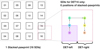 |
Fig. 1. Left panel: representation of a stacked pawprint (black solid line). The numbers refer to the detector identifications, while the dashed red square defines the total area mapped by detector 16 (DET16) when the six stacked pawprints are merged together. Right panel: schematic pattern of DET16 SDI in the six stacked pawprints. Colors and numbers denote the order and position in which the six exposures are taken. The dotted red square refers to the total field of view covered by the mosaic of the six SDIs, while DET-left and DET-right define the total area mapped by positions 1 + 2 + 3 and 4 + 5 + 6, respectively. |
The offsets pattern between the six positions was properly defined in order to get a nearly homogeneous sky coverage of ∼1.5 × 1.2 deg, called the tile. The right panel of Fig. 1 shows a schematic view of the offset pattern for any given SDI of the stacked pawprint. In summary, a single tile is composed of 16 × 6 SDIs (i.e., a stacked pawprint ×6 positions), per epoch, per filter.
The exposure time per pawprint and epoch was only 4 s for Ks and 2 × 6 s for J. With this strategy almost every pixel within a tile gets exposed at least twice, yielding an effective exposure time of 8 s for Ks and 24 s for J band for the stacked pawprints. However, the overlap areas between stacked pawprints and edges of the tiles had 2–6 times higher exposures causing the noise distribution within a tile to vary strongly with position on the sky. For this reason we decided to work on the stacked pawprint images (i.e., average of the two jittered exposures at each pawprint position), rather than using the final tile images. These images are available for download at Cambridge Astronomy Survey Unit (CASU2), after the corresponding raw science and calibration frames are processed by the VISTA data flow system pipeline (v1.3 Lewis et al. 2010). For a more detailed description see Saito et al. (2012a).
Figure 2 shows schematically the bulge area covered by the observations, and the official VVV tiles numbering also used in this work. Tiles for which two epochs in J and Ks have been used are highlighted in green, whereas those in blue have been obtained by using one epoch only. In principle, we could have used two epochs for all 196 tiles because they have been observed twice in J band and over 290 times in Ks. However, to obtain color-magnitude diagrams (CMDs) as deep and accurate as possible all images in the two bands must have similarly good image quality (IQ).
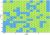 |
Fig. 2. VVV survey bulge area and tile numbering. The color-coding refers to the number of epochs used to construct the photometric catalog of each tile: green for two epochs and blue for only one epoch. |
Therefore, for all tiles we first selected the J and Ks best IQ epoch. Then, we used a second epoch only in those cases for which the second epoch in J had IQ similar (i.e., within 0.2″) to the second-best IQ epoch in Ks. Only 65% of the tiles satisfies this selection criterion. The average IQ of the selected images is 0.75″ ± 0.1 and 0.54″ ± 0.043 for J and Ks band, respectively. The complete list of stacked pawprint images used in this work amounts to 3912 (see Table A.1), which correspond to a total of 62592 SDIs (3912 × 16 = 62592 SDIs).
3. Data reduction
The bulge region studied here is characterized by a very high star density, especially close to the Galactic plane (|b| < 3°, ≳1500–3000 stars per arcmin2); therefore, to obtain accurate stellar photometry we used PSF fitting algorithms on each SDI independently. Each SDI has its own PSF, and it is thus expected to represent an independent photometric system (i.e., zero points). To obtain the final photometric catalog of any given tile we must first calculate and apply an internal detector-by-detector photometric calibration, and then combine all the SDI catalogs together. In addition, we need to assess the photometric and systematics errors affecting the derived magnitudes, and the completeness level (i.e., the fraction of observed to truly present or recovered stars per color-magnitude bin).
To this end, we made use of an ad hoc customized pipeline based on DAOPHOT, ALLSTAR (Stetson 1987), and ALLFRAME (Stetson 1994) to extract the magnitudes from the SDIs. Later for quick image coordinates transformations and internal cross-matching we used DAOMASTER (Stetson 1993).
3.1. Initial parameters
The first step toward the catalog creation is to propose a set of initial parameters to the DAOPHOT routine. For this purpose we first set the gain4 and read-out noise (RON5) levels, as published in the ESO Health Check monitor for the VIRCAM instrument. From this database we have taken the closest values to the time of observation for each SDI.
From the VIRCAM user manual6 for each detector we obtained the recommended analog-to-digital unit (ADU) value corresponding to the linearity regime. However, we found that the values listed in the manual not always reflect what is observed in the SDIs, possibly because the reduction process due to dark correction, flat-fielding, read-out mode, and combination of the jittered pair frames has slightly changed the baseline counts for each FITS. In practice, this means that the ADU levels in the images never reach the saturation threshold in the user manual. Furthermore, due to the double-correlated read mode, very bright stars have a hole with near-zero counts in their center, surrounded by a somewhat smooth ring (see Fig. 3). In addition, nonlinearity deviations in the few-percent range are already present at the 10 000 ADU, but these are well known and handled by the CASU pipeline.
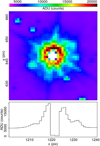 |
Fig. 3. Zoom in to a saturated star in detector 05. Top panel: heatmap of the ADU counts, while the bottom panel is an horizontal cut through the center of the star. In cases like this very bright star the fault is evident and often leads to artifacts around it, but for stars moderately within the nonlinearity and saturation regimes, the central dip is much more subtle and cannot be filtered out simply. |
Using these saturated stars as a guideline, we have defined our highest count limit to 18 500 counts, which is roughly the level at which we can still find star-like (i.e., PSF) signals, minus an arbitrary conservative margin of 1000 counts. In the case of detector 05, which has a notoriously low listed high-count limit in the instrument manual, we decided to reduce the high-count limit value to 15 500. Hereafter we refer to this as the saturation limit, even though, as stated here, it is not directly at the point of actual saturation, but when the images start being indirectly affected by it.
By taking the brightest stars in the images and measuring the approximate radius from their center at which the ADU rises well above the local sky level, we have arrived at 15 pixels to be a reasonable value for the PSF radius. This value has been adopted throughout the whole reduction procedure that leads to the catalog extraction, regardless of detector.
In order to determine the full width at half maximum (FWHM) of the stars, we proceeded as follows: (i) we selected 2000 stars by using the DAOPHOT/PICK subroutine (pick-stars) from each image, (ii) we estimated the FWHM from the profile based on the maximum number of counts and the surrounding background, and (iii) we obtained a general FWHM for the image from the median of the ensemble. We adopted a PSF fitting radius equal to the FWHM.
3.2. Calculating point spread function
To construct the PSF model for each SDI we first ran the DAOPHOT/FIND and DAOPHOT/PHOT routines and selected 450 bright isolated stars that are still well below the saturation limit (see Sect. 3.1) by using the DAOPHOT/PICK subroutine.
We then proceeded to iteratively filter out stars with a bad profile shape and bad pixels, as defined by DAOPHOT, until no star has bad pixels in its fitting radius and the final sample has no profile outliers.
Once the selection of PSF stars was made, we calculated their profile using a Moffat distribution with β = 2.5 and allowing for a quadratic XY variation of the PSF across the image. The derived PSF model was used as input parameter in the ALLSTAR routine, allowing us to remove neighboring stars, and we subsequently re-fitted the PSF profile. An iteration of five times usually led to a convergent profile for most SDIs. However, for certain problematic cases, it was necessary to reduce the counts saturation limit (i.e., in steps of 1000 ADU). The computational routine leading to the final PSF model is shown in Fig. 4.
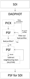 |
Fig. 4. Flow diagram of the computational routine used to obtain the PSF model of each SDI. |
3.3. SDIs mosaic and catalog calibration
As mentioned in Sect. 2, each VVV tile in each filter and epoch is a mosaic of six stacked pawprints ×16 detectors, that is 96 SDIs, most of which have negligible spatial overlap. For each VVV tile, all SDIs were processed with DAOPHOT/ALLFRAME routine following the recommendations in the “Cooking with ALLFRAME v.3” document (Turner 1997) and the PSF model as derived in Sect. 3.2. However, because ALLFRAME improves the quality of the PSF fitting only for sets of images with some spatial overlap, we ran it simultaneously on the set of three SDIs corresponding to the three vertical positions of the offsets pattern shown in Fig. 1. That is, we ran ALLFRAME on SDI 1 + 2 + 3 (×2 filters × N epochs) mosaicing into what we call DET-left, and on SDI 4 + 5 + 6, mapping into DET-right. The 16 × 2 DET-side J and Ks catalogs were first combined into 32 JKs catalogs, and then joined into a single one for each VVV field, which is what we provide to the community through the ESO Science Archive.
The absolute magnitude calibration of the photometric joint JKs catalogs is obtained through cross-correlation with the catalogs produced by CASU7 for the same set of images. Specifically, we first transformed the XY position of the detected sources in these catalogs into the absolute system RA-Dec by using the WCS recorded in each image header. Then the match with the CASU catalogs was done with STILTS (Taylor 2006), using a RA-Dec separation criterion with a tolerance of 0.5 arcsec, roughly 1.5 pixels. Overall, the match presents a natural spread of about ±(0.02 − 0.03) mag for J and usually a 50% higher for Ks (see Fig. 5). It is worth mentioning that the photometric catalogs produced by CASU and adopted here as reference system for the absolute calibration might carry a zero point calibration that is biased in denser fields. This bias may arise from possible mismatches and blends in the cross-correlation between 2MASS and VVV images performed by CASU to derive the final VVV photometric system. A thorough analysis performed on a chip-by-chip basis is not yet available; therefore, it cannot be taken into account in the present work. On the other hand, should new zero points become available in the future in the context of the VVVX survey (Minniti 2016), the calibration of the current photometric compilation can be easily improved a posteriori.
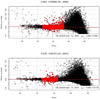 |
Fig. 5. Example plot for the CASU-ALLFRAME calibration for detector 08 of tile b249. Top panel: refers to the left side, while the bottom panel to the right side. Shown is the magnitude difference in J between CASU and ALLFRAME catalogs vs. CASU reference. The black circles follow all the matches, while the red dots mark the selected magnitude range where the zero point is calculated. The title of each plot refers to the linear fit performed on the red dots, and to the number of stars from which it is derived. Also shown in the legend is the source catalog, the estimated zero point and the corresponding uncertainty. The criterion to select the red dots is dependent on a window from which we have the minimum spread in the Δm relation. |
We also performed internal cross-checks within different pawprint images for which we have significant overlap. From these matches, the general result is a well-centered dispersion of magnitude difference, Δm, around 0 with nominal spread within 0.5σ, with an intrinsic scatter of ±0.01 mag for J and, again, about 50% higher for Ks. There are exceptions, however. For instance, the stars from detector #16 show systematically redder colors in the upper one-third of the detector (Y ≳ 1400) for all images. This is due to a known defect in the detector with filter-dependent sensitivity.
4. Completeness
The photometric completeness of the newly derived catalogs is assessed through artificial star experiments. The basic idea is to add to the SDIs synthetic stars with the observed PSF and J and Ks magnitude spanning the range observed in the data, then to re-process the entire dataset containing the artificial stars of known magnitudes by following the same procedure described in Sect. 3, but skipping the construction of the PSF model. The fraction of recovered stars with respect to those added provides an estimate of the photometric completeness.
In practice, for each DET-side JKs catalog, we first defined a color-magnitude mask covering almost the whole corresponding CMD. This mask was used to construct a uniform 2D distribution in color-magnitude space, from which we drew pairs that define the J and Ks magnitudes of the injected stars (min atlas). This allowed us to have completeness information virtually on all stars present in the observed CMD with no waste in CPU time.
The artificial stars were then spatially distributed (i.e., XY) around a grid properly customized to avoid artificially increasing the crowding (see Zoccali et al. 2003). Specifically, we used a hexagonal grid with distance between nodes of 30 pixels (∼2 × PSF radius). This allowed us to inject ∼11 000 stars per DET-side each time. We repeated the process ten times, for a total of up to ∼120 000 artificial stars per DET-side, hence ∼240 000 stars per detector.
These modified images were then processed in exactly the same way as described in Sect. 3, with the exception of both PSF models and coordinate transformations steps, which were recycled from the photometry process, rather than redefined. This produces, for each detector, two catalogs JKs (left and right). We note that since the catalogs themselves have joint JKs, that is, there is no measure in one filter without the other, the final product is a completeness value that is a function of both magnitudes: p = p(J, Ks). Finally, we cross-correlated these catalogs to the injection ones using STILTS, with a separation criterion in XY of at most 1.5 pixels (similar to the calibration run), providing us now with a recovered magnitude mrec match to the corresponding min.
We consider a star as recovered if |min − mrec| < 0.75 mag for each filter (see Sollima et al. 2007). Thus, the final completeness value p(J, Ks) is simply defined as the ratio between the number of recovered stars and the number of injected stars per (J − Ks)–Ks bin, where the latter has been defined as 0.14 × 0.13 mag2.
We note that the completeness in general is different from one detector to another, with nominal ±0.2 variations around the p = 0.5 level, regardless of actual stellar density. In addition to the p(J, Ks) values, the completeness experiments provide an estimate of the total uncertainty (systematic and photometric) of the system. This estimate comes from a fourth-degree polynomial fit to the dispersion of min − mrec per magnitude bin, and we will henceforth refer to it as the combined errors ΔJ and ΔKs.
Finally, in the available technical documentation at the CASU website8 several known issues are highlighted regarding the VISTA image quality. Most of them are either unavoidable or resolved by the time of the observations, but there are two precautions we thought we should take: we did not include detectors 04 and 16 in the completeness analysis. In the case of detector 04, the problem is mild and not always present, but we decided to exclude it. For detector 16, however, the defect is persistent and too hard to correct effectively.
5. Final photometric catalogs
The final product of the procedure described in the previous sections is a compilation of 196 photometric catalogs, one for each VVV bulge field (see Fig. 2) covering a total of ∼300 deg2 around the Galactic center. For each star detected in a given tile the catalog provides: the equatorial and galactic coordinates [RA, Dec, l, b]; the magnitudes (in the VVV photometric system) with the corresponding photometric and combined errors [J, Ks, σJ, σKs, ΔJ, ΔKs]; the completeness [p(J, Ks)]; the extinction [E(J − Ks), σE(J − Ks)], and dereddened magnitudes [J0, Ks0], as newly derived in Surot et al. (in prep.); some parameters describing the quality of the PSF fit (sharpness, χ2); the number of times a particular star was detected (rep); and a binary (i.e., base 2) flag tracing the detector(s) of origin. The binary flag can be used to refine a posteriori the photometric zero points should a new calibration based on VVVX data demonstrate the need for zero point change (see Sect. 3.3).
It is worth mentioning that to properly assess the photometric quality of each catalog one should not exclusively use the tabulated photometric errors (i.e., σJ, σKs), but rather the combined errors (ΔJ, ΔKs) described in Sect. 4. As we show in Fig. 6, the combined effect of systematics and photometric uncertainties produces a spread in the recovered versus injected magnitudes (black solid line) that is considerably larger than expected from the photometric error alone (colored points) for stars outside the 16 ≳ Ks ≳ 13 region. In addition, Fig. 6 evidences the known issue related to the saturation or nonlinearity of bright stars in the VVV Ks-band images (Ks ≲ 12). This problem is also present in the J band, but the uncertainties up to J ∼ 10 are well in line with an exponential error profile, from both photometric and simulated sources.
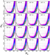 |
Fig. 6. Photometric error profile for a sample field (b249). The 2D histogram in each panel displays the σKs vs. Ks distribution of detected stars within a given detector (labeled in each panel). The color-coding indicates the density in each 2D histogram, from low (magenta) to very high (dark red) relative densities. The split or broadened sequences are due to the error mitigation in overlapping areas of a side ensemble. Detections in overlapping areas have smaller uncertainty. The black solid line refers to the combined errors: ΔKs vs. Ks, as calculated from the completeness experiments (except for detectors 04 and 16, for which no completeness is available). |
The provided χ2 and sharpness (s) values can be additionally used to flag and filter out poor and/or false detections from the catalog. The χ2 refers to the quality of the star PSF fitting, and its value should be distributed around 1 (i.e., χ2 = 1 is a perfect fit, and any value far from 1 is a poor fit). The sharpness (s) provides a measurement of how round (s = 0) the detection looks in the image.
The photometric catalogs provided here include a photometric error cut so that stars in the catalogs have σ < 0.5 mag in both J and Ks, but no cuts applied based on the quality of fit of the PSF, other than those inherent to the DAOPHOT/ALLFRAME extraction process.
The CMDs shown in Fig. 7, however, do include a number of quality filters, described in Surot et al. (2019), aimed at rejecting any detections that are unlikely to be real stars. Those selections are conservative enough so that they do not affect the catalog completeness provided here. It should be kept in mind that stronger selections that might produce thinner or better defined sequences on the CMD might significantly change the completeness, and should therefore be applied with caution when studying star counts.
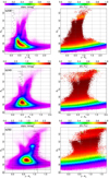 |
Fig. 7. Hess diagram of the eight selected tiles with typical color and magnitude errors shown as crosses at their respective Ks reference level (left panel), and corresponding photometric completeness map, averaged for all detectors except 04 and 16 (right panels). The VVV name of the field is labeled in each plot. |
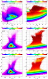 |
Fig. 7. continued. |
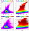 |
Fig. 7. continued. |
6. Derived color-magnitude diagrams
The entire photometric dataset is very extensive and diverse, and depends mainly on the stellar density and extinction of each field. Therefore, we show here the derived CMDs and corresponding average completeness maps only for a sample of eight tiles sparsely distributed across the bulge area (see Table 1). The fields have been selected through the relative comparison of their CMDs to easily show how the quality of the photometry varies along the bulge minor axis or at large longitudes.
Position and average color excess of the tile sample for which we show the derived CMDs.
The CMD of each tile routinely includes between 1 and 5 million stars; therefore, in order to avoid saturation in the point-scatter plots, in this work we always use Hess diagrams. Figure 7 shows the observed CMDs and completeness maps of the selected fields.
With the exception of tile b333, the common features of all CMDs are the well-defined bulge red giant branch (RGB-; reddest vertical sequence Ks ≳ 16), the bright portion of the main sequence (MS) of the disk (bluest vertical sequence Ks ≳ 16), the bulge RC (stellar overdensity along the brightest portion of the bulge RGB and generally between 14 > Ks > 12), the brightest end of the evolved disk population (vertical plume departing from the RGB toward the blue in the CMD at Ks ≲ 11, but merging with the bulge MS below that limit), and the bulge MS that overlaps with the faint portion of the disk MS. Also noteworthy are the incomplete upper RGB and the mostly missing asymptotic giant branch (AGB) due to the saturation and nonlinearity limitations.
The color spread of all sequences in the bright part of the CMD (Ks ≲ 16) is mostly caused by the differential reddening, metallicity spread, and distance depth, whereas at faint magnitudes the photometric and systematic errors become predominant, smearing out the color of MS stars over a broad magnitude range. The photometric limit is quite constant (Ks ∼ 19.5) within the sample tiles; however, as expected because of the different crowding and extinction, the photometric completeness varies substantially between the fields. For Ks ≲ 12 there is a sizable dip in completeness, with a sharp drop to zero for Ks ≲ 9. The bulge MS-TO is close to the hot spot (i.e., the densest area in the Hess diagrams); however, due to the superposition of young disk MS and the increasing dispersion, it is impossible to ascertain this evolutionary phase easily. That said, in Surot et al. (2019) we successfully demonstrated that the determination of the stellar age by means of the MS-TO luminosity is feasible, providing that enough attention is paid to the observational effects.
Fields b208, b249, and b333 deserve special attention because, given their location, the derived CMDs show peculiar features. Specifically, in the CMD of b208 we can identify the local K and M dwarf sequence as the vertical plume (Ks ≳ 16, (J − Ks) ∼ 0.8), redder than the bright disk MS and bulge RGB. This sequence is usually only evident in the outskirts of the bulge area, at very great heights from the plane (i.e., b ≲ −8°, see also Saito et al. 2012b). Moving toward the center, because of increasing reddening and stellar density, the local dwarf sequence progressively disappears because it is swallowed by the bulge RGB.
Tile b249 is particularly interesting because it is located in the region where the X-shape of the bulge is evident. From the derived CMD we can observe the presence of two well-separated RC (i.e., two apparent overdensities along the RGB at Ks ∼ 12.9 and Ks ∼ 13.2), which are the signatures of two southern arms of the X-shape structure crossing the line of sight (McWilliam & Zoccali 2010; Nataf et al. 2010; Saito et al. 2011; Wegg & Gerhard 2013; Ness & Lang 2016).
Tile b333 is also peculiar because it is located on the Galactic center region, and thus it is the most heavily reddened field in our sample (i.e., 0.7 ≲ AKs ≲ 2.4, Surot et al., in prep.). The derived CMD is the shallowest in the sample, and barely covers the entire RC population with a 50% completeness level. We note that the peculiar completeness trend (see Fig. 7) for b333 is due to a combination of many factors such as (i) the average per color-magnitude bin in this summary plot; (ii) the differences in completeness between detectors; (iii) the high differential and absolute extinction; and (iv) the rapidly declining J completeness for red stars. Finally, because the high extinction affects mostly only the bulge, the blue plume corresponding to the intervening evolved disk stars is clearly traceable in the CMD (see vertical sequence in the range 1 ≲ (J − Ks)≲2.5 and 8 ≲ Ks ≲ 12). In this respect, for studies of the evolved disk populations along the bulge line of sight, the innermost tiles affected by strong reddening are ideal because the bulge-disk (background-foreground) separation is quite clear.
7. Overview of the global photometry
The new photometric database, which contains nearly 600 millions stars, is one of the most accurate and complete censuses of the stellar population in the Milky Way bulge. This photometric database represents a valuable asset for the whole community, enabling different studies ranging from accurate star counts to stellar age determinations. It is also very useful in the context of upcoming massive spectroscopic surveys (e.g., MOONS, 4MOST) in the Milky Way by providing homogeneous catalogs for target selection over large area. All catalogs are available for download at the ESO Science Archive9 as part of the MW-BULGE-PSFPHOT release, along with a set of figures (i.e., completeness map, stellar density map, Hess diagram) that describe the main properties of the entire photometric compilation, and provide a quick look at the global bulge morphology and stellar content.
Figure 8 gives an overview of the global photometric completeness as a function of the position within the bulge, in the form of the mean Ks and Ks0 (Ks corrected for extinction from Surot et al., in prep.) magnitudes of the stars at the 50 ± 3% completeness level. By providing a global view of the photometric quality as a function of the star magnitude and position, the maps in Fig. 8 help us to quickly understand the potential and usefulness of the photometry according to the type of studies that we are interested in.
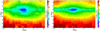 |
Fig. 8. Observed mean Ks (left panel) and reddening-corrected Ks0 (right) magnitude of stars with ∼50% completeness level (p = 0.50 ± 0.03) across the whole bulge area studied in this work. Each measurement comes from the average magnitude per individual detector per tile, where the position in the sky is set to be the middle of each detector field of view. |
For instance, for studies addressing the age determination a good sampling of the old MS-TO region is needed. Considering that for a 10 Gyr population of solar metallicity at the distance of the bulge (i.e., 8 kpc), the MS-TO is expected at Ks0 ∼ 17; by looking at the reddening-corrected completeness map (Fig. 8, right panel), we can quickly determine that, with some exceptions at l = ±10°, any field within |b| ≲ 3.5° is likely not complete enough for stellar dating. Therefore, we should either discard or treat with particular caution any results derived from such regions. On the other hand, if the science goal is to study and make a census of the RC or bright RGB populations (Ks < 14), then the photometric catalogs of all but the two most central tiles of the bulge are adequate.
As expected the overall completeness of the derived photometry increases when moving from the center outward because of the decreasing extinction and stellar density (i.e., confusion). The morphology of the bulge emerging from the completeness map closely resembles the boxy-peanut shape that is pictured in the stellar maps shown in Fig. 9. Some Galactic globular clusters located in the VVV area reveal themselves in Fig. 9 as blue and cyan small dots because of their locally higher stellar density.
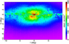 |
Fig. 9. Stellar density map of the whole bulge area as derived by counting all stars with Ks < 16. Duplicates have been addressed by counting stars in the first tile, while subsequent tiles are added excluding overlaps with adjacent fields. |
To provide a global and quick view of the stellar content within the VVV area, in Fig. 10 we show the CMD obtained by stacking together all 196 tiles (i.e., from b201 to b396) with ∼580 million sources, and accounting for the ∼10% global overlap between tiles. In the [Ks vs. (J − Ks)] plane (left panel of Fig. 10) the effect of the strong reddening is clearly evident, smearing the stars’ color over a huge range (i.e., −1 ≲ (J − Ks) ≲ 6), and making the RGB and RC sequences very blurred and hard to identify. On the other hand, when we correct the photometry by using the reddening map and the extinction law from Surot et al. (in prep.) shown in right panel of Fig. 10, the sequences of the evolved bulge stellar populations stand out clearly. We note that the color spread in the blue part of the CMD at Ks0 ≲ 16 is not representative of the actual spread in color of disk stars because it is the result of applying the bulge extinction correction to the bright MS disk stars along the line of sight that, unlike background bulge stars (and a portion of the disk stars), are not affected by the entire amount of intervening dust. In other words, the high extinction is confined mostly within the bulge only and not between us and the disk as shown in 3D extinction maps (e.g., Schultheis et al. 2014; Chen et al. 2019).
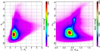 |
Fig. 10. Hess diagram of all 196 tiles stacked together in the observed [Ks, J − Ks] plane (left panel), and dereddened [Ks0, (J − Ks)0] plane (right panel) by using the color-excess map and the extinction law from Surot et al. (in prep.). The CMDs comprise nearly 600 million stars. |
Finally, due to the high differential extinction and distance depth, for detailed study of the stellar populations along the bulge line of sight Fig. 10 should not be used, but instead we suggest to consider smaller CMDs obtained within smaller sub-regions.
8. Applications
To demonstrate the tremendous potential inherent to this new photometric dataset in what follows we present examples of possible applications.
8.1. Tracing the RC star distribution
As has been well known for a long time, RC stars are very useful standard candles because their magnitude variation as a function of age and metallicity is accurately predicted by stellar evolution models (Salaris & Girardi 2002). In addition, because RC are rather bright stars, and because they are easily recognizable in the CMD plane (especially in the near-IR domain), over the years they have been extensively used for a variety of studies aimed at characterizing the bulge morphology and structure (see Wegg & Gerhard 2013; Valenti et al. 2016, and references therein), deriving reddening maps (e.g., Gonzalez et al. 2012, and references therein), and addressing the bulge age because the RC distribution provides an anchor when comparing CMDs of different fields (Zoccali et al. 2003; Valenti et al. 2013; Surot et al. 2019).
This accurate PSF photometry enables tracing the RC population across the whole VVV area. To detect the mean magnitude of the RC population across the surveyed area we have adopted a procedure very similar to that previously done by Nataf et al. (2011), Gonzalez et al. (2012), Wegg & Gerhard (2013), and Valenti et al. (2016). Specifically, we start by making an educated color-magnitude cut in the CMD so as to include evolved stars only (e.g., RGB, and RC) down to the magnitude and color levels where their sequence is still distinguishable from the bright MS of the disk (see left panel in Fig. 11). Then we estimate the Ks-magnitude star density with a narrow enough Gaussian kernel so as to not introduce extra dispersion (i.e., very similar to luminosity function histogram, but without depending on the arbitrary choice of a starting bin position). We fit the luminosity function derived in this way with a fourth-degree polynomial10 by excluding the magnitude region around the RC, where there is evident contribution from any localized overdensities (i.e., RCs and RGB bumps). By subtracting the fit to the RC region, the residual corresponds to the distribution of RC and RGB bump stars only. Finally, to trace the RC population in terms of mean magnitude and star counts we fit the residual with Gaussians (see right panel in Fig. 11).
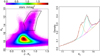 |
Fig. 11. Example of the adopted procedure to trace the RC distribution in a typical field where the X-shape of the bulge is detected (see text). Left panel: observed Hess diagram of tile b249, with a black polygon acting as the selection window used to isolate RC and RGB stars, and to construct the corresponding luminosity function reported in the right panel. The black cross shows the final estimate of the mean RC position, together with its effective width in color and magnitude. Right panel: kernel estimate of the selected RC and RGB luminosity function, not corrected for completeness (black solid line). Also plotted are the fit to the RGB distribution (violet line), and three Gaussian components used to fit the RCs (apricot and cyan) and RGB-bump (magenta). The global fit using all components is shown as a dashed red line. In this example the mean and σ of the Gaussians component are Ks = 12.82 ± 0.21 mag and 13.36 ± 0.22 mag for the RC, and 13.86 ± 0.28 mag for the RGB bump. In this exercise, no reddening or completeness correction has been applied. |
Because of the bulge’s X-shape, we know that some fields (|b|> 4 ° ,|l| ≲ 4°) show a prominent bimodality in the RC profile; therefore, in those regions we have opted to use at least three Gaussians to fit the RC profile: two for the RC and one for the RGB bump. It is worth mentioning that in principle, in the fields showing the split of the RC we should also expect two RGB bumps. However, because the luminosity of RGB bump corresponding to the brightest RC (i.e., the southern arm of the X-shape closest to us) overlaps with the luminosity range spanned by the second fainter RC, its detection and proper characterization is usually very hard. In fact, as clearly predicted by stellar evolution theory (Renzini & Fusi Pecci 1988) the RGB bump is considerably less populated than the RC. Nataf et al. (2011) estimates that in the bulge the RGB bump population makes up ≲30% of the RC stars.
To provide two examples of possible uses of the RCs that enable the study of the global bulge structure and morphology, here we show the stellar density (Fig. 12) and surface magnitude (Fig. 13) maps. The stellar density map is derived by combining the RC distribution from Valenti et al. (2016; for the region |b| ≤ 4°) and from this study (for the outer regions). As described in Valenti et al. (2016), the bulge density map clearly shows the expected boxy-peanut morphology, with increasing star density toward the center. In addition, the observed star count asymmetry along the bulge minor axis (i.e., higher density at negative longitudes) is consistent with the presence of a bar that has its close side at positive longitude.
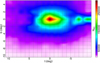 |
Fig. 12. Density map in the Galactic longitude-latitude plane based on RC star counts. Star counts for the region at |b| ≤ 4° are taken from Valenti et al. (2016), whereas those for the outer region are from this study. |
The surface magnitude profile in Fig. 13 is obtained by using the RC star counts shown in Fig. 12 and the mean intrinsic magnitude of the RC at any given line of sight (i.e.,  observed in each tile), under the assumption that for complex stellar systems older than 2–3 Gyr, the contribution of the RC population to the total luminosity is 12% (Maraston 2005).
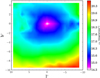 |
Fig. 13. Intrinsic (i.e., reddening corrected) surface Ks magnitude map in the Galactic longitude-latitude plane. |
Here the RC stars are used as tracers of the intermediate to old populations, which should exclude most of the disk contamination, effectively producing maps that trace instead the density of stars and surface magnitude profile in the bulge alone.
8.2. Gaia versus VVV
The cross-match between this VVV photometry and the Gaia DR2 catalog (Gaia Collaboration 2018) potentially allows us to combine the photometric and kinematic (i.e., proper motions) properties of the stellar population over most of the bulge extension. However, because of the extinction and the crowding, in practice in some bulge regions Gaia data is severely limited.
In what follows, by using the photometric completeness of our catalogs, we assess how well Gaia is able to sample the bulge stellar population. Specifically, in Fig. 14 we show the combined Gaia-VVV CMDs of four selected fields representative of different level of extinction and crowding. In the outer bulge regions (see the CMD of tile b221 in Fig. 14), Gaia data samples the bulge population down to ∼1.5 mag below the old MS-TO (i.e., Ks ∼ 17), hence we can use the stars proper motions to separate the bulge component from the intervening disk population along the line of sight allowing us to date the bulge stars by means of the MS-TO luminosity. At the latitude of Baade’s Window (i.e., b ∼ −4°; see CMD of tile b278 in Fig. 14), the Gaia photometry is already no longer deep enough to enable any kind of age study being highly incomplete at the MS-TO level. On the other hand, the RC bulge stellar population is properly sampled by Gaia throughout most of the VVV area with the exception of the innermost ∼ ± 1.5° across the Galactic plane. At b ∼ −1°, the quality of the Gaia photometry is highly variable because of both crowding and reddening. Only when the latter is still relatively weak (i.e., for E(J − Ks)≲1.5) is Gaia able to sample the RC population. This is clearly evident when we compares the CMD of the two fields b320 and b326 (see Fig. 14), which turn out to be very different even though the fields are located at the same latitude. Although b326 is in a much less crowded region than b320 (see the RC star density map in Fig. 12), the combined Gaia-VVV CMD of b326 barely samples the RC distribution because of the strong reddening. It should be noted that the limitations of Gaia in this region could be improved dramatically with LSST mapping the bulge (Gonzalez et al. 2018b).
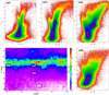 |
Fig. 14. CMDs of four VVV fields in the [Ks, BP − BR] plane as obtained by cross-matching the Gaia DR2 and this new VVV photometry (upper and lower right panel). The position of the four fields is displayed on the new bulge reddening map of Surot et al. (in prep., lower left panel). |
9. Summary
We provided a detailed and comprehensive census of the Milky Way bulge’s stellar populations by releasing new accurate photometric catalogs of the central ∼300 deg2. The photometric database, containing nearly 600 millions stars, consists of 196 catalogs obtained by performing PSF fitting photometry of multi-epoch J and Ks VVV images. Extensive artificial star experiments conducted on all 3912 images allowed us to properly assess the completeness and accuracy of the photometric measurements. With limiting magnitudes Ks ≈ 20 and J ≈ 21, this new photometric compilation allows us to characterize the evolved and un-evolved stellar population of the bulge over most of its extension. In particular, the RC stellar population is properly sampled with a photometric completeness ranging from nearly 100% to 70% throughout the VVV bulge area, with the exception of the innermost field close to the Galactic center where the completeness drops to 50%.
The photometry is accurate and deep enough to sample the old MS-TO across the whole outer bulge region (i.e., |b| ≳ 3.5°) with over ∼50% completeness, hence enabling studies of stellar ages and star formation history reconstruction based on synthetic CMD fitting techniques (see, e.g., Surot et al. 2019).
Finally, the entire photometric dataset is publicly available to the whole community at the ESO Science Archive11, as part of the MW-BULGE-PSFPHOT release.
Initially only available within the VVV team.
Close to the instrumental PSF size, thus the best IQ that VIRCAM can deliver.
Using the provided fitsio_cat_list program by CASU at http://casu.ast.cam.ac.uk/surveys-projects/software-release
2.14 − 0.635x + 0.0701x2 − 0.00362x3 + 8.34 × 10−5x4.
Acknowledgments
We thank the referee for the comments that helped us to improve the quality of the paper. FS, EV, and MR acknowledge the support from the Excellence Cluster “Origins and Structure of the Universe”. The simulations have been carried out on the computing facilities of the Computational Center for Particle and Astrophysics (C2PAP). Support for MZ and DM is provided by the BASAL CATA Center for Astrophysics and Associated Technologies through grant AFB-170002, and the Ministry for the Economy, Development, and Tourism’s Programa Iniciativa Científica Milenio through grant IC120009, awarded to Millenium Institute of Astrophysics (MAS). MZ acknowledges support from FONDECYT Regular 1150345. DM acknowledges support from FONDECYT Regular 1170121. This research made use of Astropy, a community-developed core Python package for Astronomy (Astropy Collaboration 2013, 2018), R: A language and environment for statistical computing (R Core Team 2017), as well as several packages (akima: Akima & Gebhardt 2016, gplots: Warnes et al. 2016, spatstat: Baddeley et al. 2015).
References
- Akima, H., & Gebhardt, A. 2016, akima: Interpolation of Irregularly and Regularly Spaced Data, R package version 0.6-2 [Google Scholar]
- Alonso-García, J., Minniti, D., Catelan, M., et al. 2017, ApJ, 849, L13 [NASA ADS] [CrossRef] [Google Scholar]
- Alonso-García, J., Saito, R. K., Hempel, M., et al. 2018, A&A, 619, A4 [NASA ADS] [CrossRef] [EDP Sciences] [Google Scholar]
- Astropy Collaboration (Robitaille, T. P., et al.) 2013, A&A, 558, A33 [NASA ADS] [CrossRef] [EDP Sciences] [Google Scholar]
- Astropy Collaboration (Price-Whelan, A. M., et al.) 2018, AJ, 156, A123 [NASA ADS] [CrossRef] [Google Scholar]
- Baddeley, A., Rubak, E., & Turner, R. 2015, Spatial Point Patterns: Methodology and Applications with R (London: Chapman and Hall/CRC Press) [CrossRef] [Google Scholar]
- Chen, B.-Q., Huang, Y., Yuan, H.-B., et al. 2019, MNRAS, 483, 4277 [NASA ADS] [CrossRef] [Google Scholar]
- Gaia Collaboration (Brown, A. G. A., et al.) 2018, A&A, 616, A1 [NASA ADS] [CrossRef] [EDP Sciences] [Google Scholar]
- Gonzalez, O. A., Rejkuba, M., Zoccali, M., et al. 2012, A&A, 543, A13 [NASA ADS] [CrossRef] [EDP Sciences] [Google Scholar]
- Gonzalez, O. A., Minniti, D., Valenti, E., et al. 2018a, MNRAS, 481, L130 [NASA ADS] [CrossRef] [Google Scholar]
- Gonzalez, O. A., Clarkson, W., Debattista, V. P., et al. 2018b, ArXiv e-prints [arXiv:1812.08670] [Google Scholar]
- Lewis, J. R., Irwin, M., & Bunclark, P. 2010, ASP Conf. Ser., 434, 91 [NASA ADS] [Google Scholar]
- Maraston, C. 2005, MNRAS, 362, 799 [NASA ADS] [CrossRef] [Google Scholar]
- McWilliam, A., & Zoccali, M. 2010, ApJ, 724, 1491 [NASA ADS] [CrossRef] [Google Scholar]
- Minniti, D. 2016, Galactic Surveys: New Results on Formation, Evolution, Structure and Chemical Evolution of the Milky Way, 10 [Google Scholar]
- Minniti, D., Lucas, P. W., Emerson, J. P., et al. 2010, Nature, 15, 433 [Google Scholar]
- Nataf, D. M., Udalski, A., Gould, A., Fouqué, P., & Stanek, K. Z. 2010, ApJ, 721, L28 [NASA ADS] [CrossRef] [Google Scholar]
- Nataf, D. M., Udalski, A., Gould, A., & Pinsonneault, M. H. 2011, ApJ, 730, 118 [NASA ADS] [CrossRef] [Google Scholar]
- Nataf, D. M., Gonzalez, O. A., Casagrande, L., et al. 2016, MNRAS, 456, 2692 [NASA ADS] [CrossRef] [Google Scholar]
- Ness, M., & Lang, D. 2016, AJ, 152, 14 [NASA ADS] [CrossRef] [Google Scholar]
- R Core Team 2017, R: A Language and Environment for Statistical Computing, (Vienna, Austria: R Foundation for Statistical Computing) [Google Scholar]
- Renzini, A., & Fusi Pecci, F. 1988, ARA&A, 26, 199 [NASA ADS] [CrossRef] [Google Scholar]
- Saito, R. K., Zoccali, M., McWilliam, A., et al. 2011, AJ, 142, 76 [NASA ADS] [CrossRef] [Google Scholar]
- Saito, R. K., Hempel, M., Minniti, D., et al. 2012a, A&A, 537, A107 [NASA ADS] [CrossRef] [EDP Sciences] [Google Scholar]
- Saito, R. K., Minniti, D., Dias, B., et al. 2012b, A&A, 544, A147 [NASA ADS] [CrossRef] [EDP Sciences] [Google Scholar]
- Salaris, M., & Girardi, L. 2002, MNRAS, 337, 332 [NASA ADS] [CrossRef] [Google Scholar]
- Schultheis, M., Chen, B. Q., Jiang, B. W., et al. 2014, A&A, 566, A120 [NASA ADS] [CrossRef] [EDP Sciences] [Google Scholar]
- Smith, L. C., Lucas, P. W., Kurtev, R., et al. 2018, MNRAS, 474, 1826 [NASA ADS] [CrossRef] [Google Scholar]
- Sollima, A., Beccari, G., Ferraro, F. R., Fusi Pecci, F., & Sarajedini, A. 2007, MNRAS, 380, 781 [NASA ADS] [CrossRef] [Google Scholar]
- Stetson, P. B. 1987, PASP, 99, 191 [NASA ADS] [CrossRef] [Google Scholar]
- Stetson, P. B. 1993, in IAU Colloq. 136: Stellar Photometry – Current Techniques and Future Developments, eds. C. J. Butler, & I. Elliott, 136, 291 [NASA ADS] [Google Scholar]
- Stetson, P. B. 1994, PASP, 106, 250 [NASA ADS] [CrossRef] [Google Scholar]
- Surot, F., Valenti, E., Hidalgo, S. L., et al. 2019, A&A, 623, A168 [NASA ADS] [CrossRef] [EDP Sciences] [Google Scholar]
- Taylor, M. B. 2006, ASP Conf. Ser., 351, 666 [NASA ADS] [Google Scholar]
- Turner, A. 1997, Cooking with ALLFRAME, version 3 (Victoria: Dominion Astrophysical Observatory) [Google Scholar]
- Valenti, E., Zoccali, M., Renzini, A., et al. 2013, A&A, 559, A98 [NASA ADS] [CrossRef] [EDP Sciences] [Google Scholar]
- Valenti, E., Zoccali, M., Gonzalez, O. A., et al. 2016, A&A, 587, L6 [NASA ADS] [CrossRef] [EDP Sciences] [Google Scholar]
- Warnes, G. R., Bolker, B., Bonebakker, L., et al. 2016, gplots: Various R Programming Tools for Plotting Data, R package version 3.0.1 [Google Scholar]
- Wegg, C., & Gerhard, O. 2013, MNRAS, 435, 1874 [Google Scholar]
- Zoccali, M., Renzini, A., Ortolani, S., et al. 2003, A&A, 399, 931 [NASA ADS] [CrossRef] [EDP Sciences] [Google Scholar]
Appendix A: VVV stacked pawprint images
VVV stacked pawprint images used in this work, together with the corresponding image quality, airmass, and ellipticity as derived by the fits header.
All Tables
Position and average color excess of the tile sample for which we show the derived CMDs.
VVV stacked pawprint images used in this work, together with the corresponding image quality, airmass, and ellipticity as derived by the fits header.
All Figures
|
Fig. 1. Left panel: representation of a stacked pawprint (black solid line). The numbers refer to the detector identifications, while the dashed red square defines the total area mapped by detector 16 (DET16) when the six stacked pawprints are merged together. Right panel: schematic pattern of DET16 SDI in the six stacked pawprints. Colors and numbers denote the order and position in which the six exposures are taken. The dotted red square refers to the total field of view covered by the mosaic of the six SDIs, while DET-left and DET-right define the total area mapped by positions 1 + 2 + 3 and 4 + 5 + 6, respectively. |
| In the text | |
|
Fig. 2. VVV survey bulge area and tile numbering. The color-coding refers to the number of epochs used to construct the photometric catalog of each tile: green for two epochs and blue for only one epoch. |
| In the text | |
|
Fig. 3. Zoom in to a saturated star in detector 05. Top panel: heatmap of the ADU counts, while the bottom panel is an horizontal cut through the center of the star. In cases like this very bright star the fault is evident and often leads to artifacts around it, but for stars moderately within the nonlinearity and saturation regimes, the central dip is much more subtle and cannot be filtered out simply. |
| In the text | |
|
Fig. 4. Flow diagram of the computational routine used to obtain the PSF model of each SDI. |
| In the text | |
|
Fig. 5. Example plot for the CASU-ALLFRAME calibration for detector 08 of tile b249. Top panel: refers to the left side, while the bottom panel to the right side. Shown is the magnitude difference in J between CASU and ALLFRAME catalogs vs. CASU reference. The black circles follow all the matches, while the red dots mark the selected magnitude range where the zero point is calculated. The title of each plot refers to the linear fit performed on the red dots, and to the number of stars from which it is derived. Also shown in the legend is the source catalog, the estimated zero point and the corresponding uncertainty. The criterion to select the red dots is dependent on a window from which we have the minimum spread in the Δm relation. |
| In the text | |
|
Fig. 6. Photometric error profile for a sample field (b249). The 2D histogram in each panel displays the σKs vs. Ks distribution of detected stars within a given detector (labeled in each panel). The color-coding indicates the density in each 2D histogram, from low (magenta) to very high (dark red) relative densities. The split or broadened sequences are due to the error mitigation in overlapping areas of a side ensemble. Detections in overlapping areas have smaller uncertainty. The black solid line refers to the combined errors: ΔKs vs. Ks, as calculated from the completeness experiments (except for detectors 04 and 16, for which no completeness is available). |
| In the text | |
|
Fig. 7. Hess diagram of the eight selected tiles with typical color and magnitude errors shown as crosses at their respective Ks reference level (left panel), and corresponding photometric completeness map, averaged for all detectors except 04 and 16 (right panels). The VVV name of the field is labeled in each plot. |
| In the text | |
|
Fig. 7. continued. |
| In the text | |
|
Fig. 7. continued. |
| In the text | |
|
Fig. 8. Observed mean Ks (left panel) and reddening-corrected Ks0 (right) magnitude of stars with ∼50% completeness level (p = 0.50 ± 0.03) across the whole bulge area studied in this work. Each measurement comes from the average magnitude per individual detector per tile, where the position in the sky is set to be the middle of each detector field of view. |
| In the text | |
|
Fig. 9. Stellar density map of the whole bulge area as derived by counting all stars with Ks < 16. Duplicates have been addressed by counting stars in the first tile, while subsequent tiles are added excluding overlaps with adjacent fields. |
| In the text | |
|
Fig. 10. Hess diagram of all 196 tiles stacked together in the observed [Ks, J − Ks] plane (left panel), and dereddened [Ks0, (J − Ks)0] plane (right panel) by using the color-excess map and the extinction law from Surot et al. (in prep.). The CMDs comprise nearly 600 million stars. |
| In the text | |
|
Fig. 11. Example of the adopted procedure to trace the RC distribution in a typical field where the X-shape of the bulge is detected (see text). Left panel: observed Hess diagram of tile b249, with a black polygon acting as the selection window used to isolate RC and RGB stars, and to construct the corresponding luminosity function reported in the right panel. The black cross shows the final estimate of the mean RC position, together with its effective width in color and magnitude. Right panel: kernel estimate of the selected RC and RGB luminosity function, not corrected for completeness (black solid line). Also plotted are the fit to the RGB distribution (violet line), and three Gaussian components used to fit the RCs (apricot and cyan) and RGB-bump (magenta). The global fit using all components is shown as a dashed red line. In this example the mean and σ of the Gaussians component are Ks = 12.82 ± 0.21 mag and 13.36 ± 0.22 mag for the RC, and 13.86 ± 0.28 mag for the RGB bump. In this exercise, no reddening or completeness correction has been applied. |
| In the text | |
|
Fig. 12. Density map in the Galactic longitude-latitude plane based on RC star counts. Star counts for the region at |b| ≤ 4° are taken from Valenti et al. (2016), whereas those for the outer region are from this study. |
| In the text | |
|
Fig. 13. Intrinsic (i.e., reddening corrected) surface Ks magnitude map in the Galactic longitude-latitude plane. |
| In the text | |
|
Fig. 14. CMDs of four VVV fields in the [Ks, BP − BR] plane as obtained by cross-matching the Gaia DR2 and this new VVV photometry (upper and lower right panel). The position of the four fields is displayed on the new bulge reddening map of Surot et al. (in prep., lower left panel). |
| In the text | |
Current usage metrics show cumulative count of Article Views (full-text article views including HTML views, PDF and ePub downloads, according to the available data) and Abstracts Views on Vision4Press platform.
Data correspond to usage on the plateform after 2015. The current usage metrics is available 48-96 hours after online publication and is updated daily on week days.
Initial download of the metrics may take a while.