| Issue |
A&A
Volume 629, September 2019
|
|
|---|---|---|
| Article Number | A37 | |
| Number of page(s) | 17 | |
| Section | Extragalactic astronomy | |
| DOI | https://doi.org/10.1051/0004-6361/201834720 | |
| Published online | 02 September 2019 | |
Assembly of spheroid-dominated galaxies in the EAGLE simulation
1
Instituto de Astronomía y Física del Espacio, CONICET-UBA, Casilla de Correos 67, Suc. 28, 1428 Buenos Aires, Argentina
e-mail: This email address is being protected from spambots. You need JavaScript enabled to view it.
2
Departamento de Ciencias Físicas, Universidad Andrés Bello, 700 Fernandez Concha, Santiago, Chile
3
Centro de Estudios de Física del Cosmo de Aragón, Plaza San Juan 1, Planta 2, 44001 Teruel, Spain
4
Donostia International Physics Center (DIPC), Manuel Lardizabal Pasealekua 4, 20018 Donostia, Basque Country, Spain
Received:
26
November
2018
Accepted:
15
July
2019
Abstract
Context. Despite the insights gained in the last few years, our knowledge about the formation and evolution scenario for the spheroid-dominated galaxies is still incomplete. New and more powerful cosmological simulations have been developed that together with more precise observations open the possibility of more detailed study of the formation of early-type galaxies (ETGs).
Aims. The aim of this work is to analyse the assembly histories of ETGs in a Λ cold dark matter cosmology, focussing on the archeological approach given by the mass-growth histories.
Methods. We inspected a sample of dispersion-dominated galaxies selected from the largest volume simulation of the EAGLE project. This simulation includes a variety of physical processes such as radiative cooling, star formation (SF), metal enrichment, and stellar and active galactic nucleus (AGN) feedback. The selected sample comprised 508 spheroid-dominated galaxies classified according to their dynamical properties. Their surface brightness profile, the fundamental relations, kinematic properties, and stellar-mass growth histories are estimated and analysed. The findings are confronted with recent observations.
Results. The simulated ETGs are found to globally reproduce the fundamental relations of ellipticals. All of them have an inner disc component where residual younger stellar populations (SPs) are detected. A correlation between the inner-disc fraction and the bulge-to-total ratio is reported. We find a relation between kinematics and shape that implies that dispersion-dominated galaxies with low V/σL (where V is the average rotational velocity and σL the one dimensional velocity dispersion) tend to have ellipticity smaller than ∼0.5 and are dominated by old stars. On average, less massive galaxies host slightly younger stars. More massive spheroids show coeval SPs while for less massive galaxies (stellar masses lower than ∼1010 M⊙), there is a clear trend to have rejuvenated inner regions, showing an age gap between the inner and the outer regions up to ∼2 Gyr, in apparent contradiction with observational findings. We find evidences suggesting that both the existence of the disc components with SF activity in the inner region and the accretion of satellite galaxies in outer regions could contribute to the outside-in formation history in galaxies with low stellar mass. On the other hand, there are non-negligible uncertainties in the determination of the ages of old stars in observed galaxies. Stronger supernova (SN) feedback and/or the action of AGN feedback for galaxies with stellar masses lower than 1010 M⊙ could contribute to prevent the SF in the inner regions.
Key words: galaxies: formation / galaxies: elliptical and lenticular / cD / galaxies: abundances / galaxies: kinematics and dynamics
Corresponding Investigator, IATE-CONICET, Laprida 927, Córdoba, Argentina.
© ESO 2019
1. Introduction
Once thought as simple systems formed in a monolithic collapse, early-type galaxies (ETGs) are currently considered complex structures likely formed by the combination of diverse physical processes such as infall and collapse, major and/or minor mergers (e.g. Burkert & Naab 2004; Bournaud et al. 2007; González-García et al. 2009; Zavala et al. 2012; Tissera 2012; Perez et al. 2013; Avila-Reese et al. 2014; Dubois et al. 2016; Rodriguez-Gomez et al. 2016, and references therein). The development of integral field spectroscopy (IFS) has allowed a deeper analysis of the SPs and interstellar medium (ISM) of galaxies and particularly of ETGs. Recent multi-object surveys such as SAMI (Croom et al. 2012) and MaNGA (Bundy et al. 2015; SDSS Collaboration 2017), and single-object ones like ALTAS3D (Cappellari et al. 2011) and CALIFA (Sánchez et al. 2012) provide more detailed information that improve our understanding of the astrophysical properties and fundamental relations of galaxies in a wide range of stellar masses and morphologies.
The construction of stellar-mass growth histories (MGHs) for a significant number of galaxies has been made possible by IFS surveys. The MGHs provide archaeological estimations of galaxy assembly. Recent observational works find a significant fraction of galaxies in the Local Universe to be consistent with an inside-out formation history as they exhibit negative age gradients (Wang et al. 2011; Lin et al. 2013; Li et al. 2015). This implies that the star formation (SF) in the inner regions occurs at earlier times than in outer regions of the galaxies. For the ETGs, it is not yet clear how they assembled and/or quenched their SF activity as a function of radius. Supernova (SN) and active galactic nucleus (AGN) feedback can contribute to regulate the SF activity in galaxies of different masses. Recent results by Argudo-Fernández et al. (2018) suggest that AGN feedback might even act in galaxies with stellar masses down to 1010 M⊙. Further, there is new evidence that suggests the action of AGN feedback in dwarf galaxies (Manzano-King et al. 2019).
Evidence for both inside-out and outside-in scenarios for ETGs has been observationally reported (Sánchez-Blázquez et al. 2007). Ibarra-Medel et al. (2016) study galaxies from the MaNGA survey (Bundy et al. 2015; SDSS Collaboration 2017) finding an inside-out scenario in star-forming and late-type galaxies. In less massive systems, there is a larger variety of behaviours in the observed MGHs. Early-type galaxies are detected as being consistent with a weak inside-out formation at later epochs. At early epochs, a slight trend from outside-in formation is found. However, the main caveat to studying ETG assembly is the determination of ages for SPs older than ∼10 Gyr. Another effect to be considered in the formation of ETGs is the contribution of old stars acquired by satellite accretion (e.g. Genel et al. 2018). The accretion of satellites could add older stars to the outer regions helping to establish an outside-in formation scenario. However, if the accreted SPs are younger than the main SPs of the principal galaxy then the opposite scenario could be set. From an observational point of view, this is yet not clearly established.
The current cosmological scenario for the formation of the structure shows that different morphologies can be associated with a variety of formation histories at a given stellar mass (De Rossi et al. 2015; Trayford et al. 2019). In particular, mergers have been shown to be able to change galaxy morphology drastically (e.g. Mihos & Hernquist 1996). During the early stages of the interactions, these processes may trigger tidal fields that drive gas inflows, producing starbursts that can feed the spheroidal component (Hernquist 1989; Sillero et al. 2017). These processes can modify the metallicity distributions, contributing to weaken the metallicity gradients as well as triggering SF (e.g. Rupke et al. 2010; Perez et al. 2013; Tissera et al. 2016; Taylor & Kobayashi 2017; Bustamente 2018). Galactic winds might be generated by stellar or AGN feedback that could transport material out of the galaxy, modifying the morphologies, the SF activity, and the chemical abundances (e.g. Gibson et al. 2013; Genel et al. 2015; Dubois et al. 2016; Tissera et al. 2019). Naab (2013) proposes a two-phase assembly history: first the action of dissipative processes that triggered in situ SF at high redshift and second, the action of dry accretion of nearby galaxies. Dry mergers have also been proposed as a mechanism responsible for the formation of ETGs, principally of the outskirts, because they contribute with old stars and small amount of gas (Genel et al. 2018). While SN feedback is a crucial process to regulating the transformation of gas into stars in galaxies, AGN feedback is also required at high stellar masses where SN feedback is not that efficient.
By analysing data from the Illustris Project (Vogelsberger et al. 2014a,b; Genel et al. 2014), Rodriguez-Gomez et al. (2016) quantify the fraction of ex-situ mass coming from major or minor mergers, finding that half of the ex-situ mass comes, on average, from major mergers. For galaxies with stellar masses ∼1010 − 1011 M⊙, the ratio between the accreted mass over the total mass shows a non-negligible scatter. They conclude that features such as morphology and halo formation time, together with the merger histories affect the fraction of ex-situ mass (e.g., at a fixed stellar mass spheroid galaxies with late halo formation have higher fractions). Consistently with studies of simulations of galaxy mergers, they find that in-situ SF lies in the centre of the galaxy, while stars accreted during mergers are found in the outer regions. Clauwens et al. (2018) study the origin of the different morphologies in central galaxies from the EAGLE simulation (Schaye et al. 2015; Crain et al. 2015). They describe how the disc and the bulge components of galaxies form. They distinguish three phases of galaxy formation. When MStar < 109.5 M⊙, galaxy evolution would be dominated by random motions, growing disorderly. In this phase, SF occurs mostly in situ, possible fed by wet mergers. When the stellar mass of galaxies is in the range 109.5 M⊙ < MStar < 1010.5 M⊙, there is also in situ SF, but in systems with disc morphologies. Finally, at higher masses, there is a transformation to more spheroid-dominated galaxies where the spheroid formation is mainly due to accretion of ex-situ stars at large radii. Furthermore, Trayford et al. (2019) analyse the morphological evolution of galaxies in the EAGLE simulation, studying the changes produced by mergers, accretion and secular evolution in galaxies as a function of redshift. They conclude that the stellar-mass fraction of spheroids increases steadily towards z ∼ 0 and that galaxies that have mergers with mass ratios larger than 1:10 tend to change their morphology from disc-dominated to spheroidal-dominated.
Recently, Rosito et al. (2018) investigate a sample of field ETGs selected from Fenix project (Pedrosa & Tissera 2015). These authors report the simulated ETGs to be able to reproduce the size-mass relation, fundamental plane (FP) and the Faber-Jackson relation (FJR) and to have formed in an inside-out fashion, in general. All the analysed dispersion-dominated galaxies have small disc components and ∼60% of them can be classified as pseudo-bulges (assuming Sérsic index lower than 2). These authors find that the spheroidal galaxies have slightly bluer colours than expected, consistent with having been recently rejuvenated. Compared to observations, the fraction of rejuvenated simulated spheroids is larger, suggesting the need for a stronger quenching mechanism. However, the MGHs obtained by Rosito et al. (2018) are in global agreement with the observational trends by Ibarra-Medel et al. (2016) that show an inside-out formation history for low-mass galaxies ETGs. For massive ETGs, all SPs seem to be coeval with a slight trend to inside-out formation. This study is based on a small number sample of galaxies (18) restricted to a typical field region of the universe, and hence it does not grant a statistical analysis which allows for a large variety of assembly histories.
In this paper, we analyse the dispersion-dominated galaxies identified in the 100 Mpc cubic volume simulation of the EAGLE project (Crain et al. 2015; Schaye et al. 2015). Hence, this galaxy sample allows us to explore a larger variety of assembly histories in comparison with Rosito et al. (2018), though the detailed modelling of subgrid physics differs. The selected EAGLE spheroid-dominated galaxies (hereafter, E-SDGs) sample comprises 508 members resolved with more than 10 000 stellar particles. In order to validate the E-SDGs, first we estimate their structural and fundamental relations and compare them with observations from ATLAS3D (Cappellari et al. 2013a,b). We also calculate the shapes and kinematic properties. Then, the MGHs as well as the metallicity properties are analysed as a function of stellar galaxy mass and the bulge-to-total mass ratio.
This paper is organised as follows. In Sect. 2, the main aspects of the EAGLE project are summarised and, in Sect. 3, we characterise the simulated galaxies via morphological decomposition, the analysis of the surface density profile and the scaling relations. In Sect. 4, we discuss the relation between shape and kinematics. Section 5 describes the MGHs. Finally, Sect. 6 summarises the results.
2. The EAGLE simulation
We analyse galaxies selected from the 100 Mpc sized box reference run of the EAGLE project, a suite of hydrodynamical simulations that follows the formation of structure in cosmological representative volumes, all of them consistent with the current favoured Λ cold dark matter cosmology (Crain et al. 2015; Schaye et al. 2015). These simulations include: radiative heating and cooling (Wiersma et al. 2009), stochastic SF (Schaye & Dalla Vecchia 2008), stochastic stellar feedback (Dalla Vecchia & Schaye 2012) and AGN feedback (Rosas-Guevara et al. 2015). The AGN feedback is particular important for the evolution of SF activity in massive ETGs. An Initial Mass Function (IMF) of Chabrier (2003) is used. A more detail description of the code and the simulations is given by Crain et al. (2015) and Schaye et al. (2015).
The adopted cosmological parameters are: Ωm = 0.307, ΩΛ = 0.693, Ωb = 0.04825, H0 = 100 h km s−1 Mpc−1, with h = 0.6777 (Planck Collaboration I 2014; Planck Collaboration XVI 2014). The 100 Mpc sized box reference simulation, so called L100N1504, is represented by 15043 dark matter particles and the same initial number of gas particles, with an initial mass of 9.70 × 10⁶ M⊙ and 1.81 × 10⁶ M⊙, respectively (Schaye et al. 2015). A maximum gravitational softening of 0.7 kpc is adopted.
We use the publicly available database by McAlpine et al. (2016).
3. The selected sample of galaxies
In this work, we use the sample of 7482 central galaxies selected by Tissera et al. (2019) from the EAGLE galaxy catalog of L100N1504. To diminish numerical resolution artefacts, we only analyse those galaxies resolved with more than 10 000 stellar particles within 1.5 Ropt1 Thus, the selected EAGLE galaxy subsample has 1721 members with masses in the range ∼[0.22 − 16.7]×1010 M⊙, where the total stellar mass is defined as the sum of the bulge and disc stellar-mass components (defined as below) within 1.5 Ropt2.
The morphological classification is performed by applying the method described by Tissera et al. (2012). For each stellar particle, we use the parameter ϵ = Jz/Jz, max(E) where Jz is the angular momentum component in the direction of the total angular momentum and Jz, max is the maximum Jz over all particles at a given binding energy (E). Those particles with ϵ > 0.5 are associated with the disc component, whereas the rest of them are considered part of the spheroid component. In order to discriminate between the bulge (also called spheroid) and the stellar halo, the particle binding energy is used so that the most bounded particles are assigned to the bulge. We assume the minimum energy of the particles at half of Ropt as the E threshold (Tissera et al. 2012).
This decomposition allows the definition of the bulge-to-total mass ratios (B/T that takes into account only the bulge and disc components), which are used to select galaxies according to their morphology. In Fig. 1, we show the distribution of B/T ratios for our EAGLE sample. Following previous works (Pedrosa & Tissera 2015; Rosito et al. 2018; Tissera et al. 2019), we adopt B/T = 0.5 to separate disc-dominated from spheroid-dominated galaxies (DDGs and SDGs, respectively).
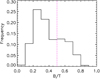 |
Fig. 1. Distribution of B/T ratios for selected EAGLE galaxies. Only those galaxies with B/T > 0.5 are classified as SDGs (dashed magenta line). |
The SDG sample comprises 508 members and will be hereafter called E-SDGs. As can be seen from Fig. 1, all simulated galaxies have a stellar disc component, regardless of the size of spheroidal system. The total stellar masses, defined by adding the bulge and the disc components, are in the range [0.4, 14]×1010 M⊙.
In order to analyse the scaling relations, we also estimate the stellar projected half-mass radius, Rhm. The projection is peformed onto the xy-plane, where z is the direction of the total angular momentum. We also obtain the three dimensional half-mass radius, hereafter called  .
.
For the SPs in each E-SDG, we measure the specific star formation rate (sSFR) calculated with star particles younger than 0.5 Gyr, the mass-weighted stellar age, the velocity dispersion (σ), and the average rotational velocity (V) within the Rhm. The median chemical abundances: [Fe/H], [O/Fe] and [O/H] are estimated within  .
.
3.1. Surface-mass densities
The projected stellar-mass surface density profiles on the xy-plane for both disc and spheroid components are estimated. Sérsic profiles (Sérsic 1968) are fitted for the bulges, obtaining the central surface brightness (I0), the scale radius (Rb) and the so-called Sérsic index (n) according to
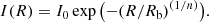
The surface density profiles of the discs are fitted with an exponential profile (n = 1) with a scale-length Rd. We consider the projected stellar-mass surface density as a proxy of the luminosity surface brightness, which is equivalent to adopting a mass-to-light ratio M/L = 1. This ratio is close to the observed one for the infrared bands and is consistent with that adopted by Rosito et al. (2018). In the case of the spheroidal components, the Sérsic profile is fitted within the radial range defined by one gravitational softening and the radius that encloses 90% of the total spheroid mass (to avoid numerical noise in the inner and very outer regions). The exponential fit to the discs is performed within the latter and the Ropt.
In Fig. 2, we show two examples of simulated galaxies with different surface density profiles. As can be seen, the profiles are well-reproduced by the Sérsic law and an exponential profile for the spheroid and disc, respectively. In the central regions, the bulge and disc components co-exist, although different behaviours are identified as can be seen from Fig. 2. In general, the discs either extend into the bulge region, following the disc exponential profiles (upper panel) or increases their surface densities so that they might reach that of the bulge (lower panel). In this case, they could also be interpreted as part of the bulge since their contribution is small. The different characteristics of the co-existence of the discs and the spheroids reflect the variety of assembly histories (e.g. Trayford et al. 2019).
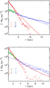 |
Fig. 2. Projected stellar-mass surface density profiles for bulge (red diamonds) and disc components (blue diamonds) of two typical simulated ETGs. The regions of the discs that co-exist with spheroid components are highlighted (green diamonds). The best-fitted Sérsic profiles for the spheroid components (solid red lines) and the exponential profiles for the discs (dashed blue lines) are also included. The bulge effective radius (Reff, calculated by using Eq. (6) in Sáiz et al. 2001), the Rhm and the Rd are depicted with red, black and blue arrows, respectively. In the upper panel, the inner disc follows the exponential profile (n ∼ 1.25) while in the lower panel, the same component follows the bulge profile (n ∼ 2.78). A variety of behaviours is detected, suggesting different contributions of processes such as collapse, mergers and secular evolution. |
Following Rosito et al. (2018), we quantified the fraction of the disc stellar mass that co-exists with the bulge component by estimating the stellar mass with ϵ > 0.5 and binding energy lower than the energy threshold adopted to define the bulges (Frot). In Fig. 3, we show Frot as a function of B/T. In order to obtain smoothed distributions, we use the Python implementation (Cappellari et al. 2013b) of the two-dimensional Locally Weighted Regression (Cleveland & Devlin 1988) method. This method generalizes the polynomial regression and has the advantage that it is not necessary to specify a function to fit a model to the data sample, being notably simply to implement. By smoothing our plots, the tendencies can be more clearly appreciated. We must bear in mind, however, that some colours may be affected by this method. We applied this method in all our scatter plots, hereafter. In Appendix B we include the figures without smoothing the distributions. We fix the colour-bar limits to the first and third quartile of the variable according to which we colour the symbols in the smoothed plots, except for the ones in Appendix A.
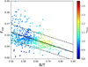 |
Fig. 3. Stellar-mass fractions Frot of the discs that co-exist with the spheroidal components as a function of the B/T ratio. Symbols are coloured according to n. A linear regression fit is included (solid black line) along with its 1σ dispersion (dashed black lines). |
Most of the E-SDGs (∼85%) have n < 2 (∼53% of the E-SDGs have n > 1) and will be classified as pseudo-bulges. These systems are expected to have been formed by a significant contribution of secular evolution (see Kormendy 2016, for a recent review). We note that other authors assumes different definitions taking into account, for example, the inner shape or just the resulting product of secular evolution in the inner part of the galactic disc (e.g. Falcón-Barroso & Knapen 2012). We decide to use n = 2 for the sake of simplicity.
As can be seen from Fig. 3, E-SDGs with large B/T ratios tend to have small Frot. This is the expected behaviour considering that more massive galaxies have larger probability to have experienced a higher rate of mergers (Rodriguez-Gomez et al. 2015), producing more classical bulges. There is only a weak trend to have slightly higher n for these galaxies. On the other hand, larger inner discs (Frot > 0.2) are found in the more discoidal E-SDGs that tend to have n ≤ 1, as expected if bulges formed from secular evolution or wet mergers (Kormendy 2016). As can be seen from this figure, at a given B/T ratio, there is a large variation of Frot, suggesting different assembly histories (i.e. different contributions of collapse, wet and dry mergers, and secular evolution for example). There is no clear trend for galaxies with n > 2 as can be seen from Fig. B.1, where the distribution has not been smoothed. The Spearman coefficient for the relation is −0.47. The linear regression yields an slope of −0.40 ± 0.04 (this error is calculated by a bootstrap method). The relation suggests that those galaxies that have larger disc components are able to extend these discs all the way to the central region (Rosito et al. 2018).
The E-SDGs show no clear correlation between B/T and n as shown in Fig. 4 (Spearman coefficient 0.09, p-value of 0.03). From Fig. 4, we can also see that those E-SDGs with larger B/T ratios have, on average, the oldest SPs (E-SDGs galaxies are coloured according to mass-weighted age of the total galaxy). We note that a fraction of E-SDGs with the larger n index tend to have slightly younger SPs, on average. This is because there is a larger fraction of young stars associated to the disc components as we will discuss in more detail in Sect. 5.
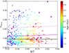 |
Fig. 4. Sérsic index (nSersic) as a function of B/T ratio for the simulated E-SDGs, coloured according to the mass-weighted average age of the galaxy stellar mass. A linear regression fit is included (solid magenta line) with its 1σ dispersion (dashed magenta line). For comparison, we also include the results by Rosito et al. (2018; magenta squares). The line nSersic = 1 is depicted in a black line. See Appendix B for the non-smoothed distribution. |
In Fig. 5, we show the mass-weighted ages as a function of the stellar mass for the E-SDGs. The colour code denotes the B/T ratios. As can be seen, there is a general trend to have more massive galaxies populated by old stars, on average, and with larger B/T ratios as expected. As one moves to more discoidal E-SDGs, the stellar ages are smaller and the galaxies are less massive. However, at a given stellar mass, there is a large variety of both morphologies and ages.
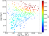 |
Fig. 5. Mass-weighted stellar age of the E-SDGs (i.e. bulge and disc SPs) as a function of stellar mass for the simulated galaxies. The symbols are coloured according to the B/T ratios. See Appendix B for the non-smoothed distribution. |
3.2. Scaling relations
In this subsection, we analyse three main scaling relations for the E-SDGs: the size-mass relation, the FJR (Faber & Jackson 1976) and the FP (Faber et al. 1987; Dressler et al. 1987; Djorgovski & Davis 1987), and compare them with observations. To estimate these scaling relations we use the Rhm as the characteristic size for the simulated galaxies.
Size-mass relation
The size-mass relation for the E-SDGs and those obtained from different observational works are shown in Fig. 6. We compare simulated size-mass relation with the observational trends reported by Mosleh et al. (2013) and Bernardi et al. (2014). For the former, we take those corresponding to ETGs (Table 1 in Mosleh et al. 2013) and for the latter, we choose the case of a single Sérsic profile (their Table 4). We also compare our results with the observations from ATLAS3D Project that consists of a sample of 260 nearby ETGs (Cappellari et al. 2011, 2013a). The stellar masses are calculated from the luminosities given by Cappellari et al. (2013a, Table 1) and by using the mass-to-light ratios of Cappellari et al. (2013b, Table 1) for a Salpeter IMF (Salpeter 1955). The corresponding correction to transform Salpeter estimated stellar masses to the Chabrier IMF (Chabrier 2003) has been applied.
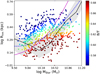 |
Fig. 6. Mass-size relation estimated for E-SDGs. Symbols are coloured according to their B/T ratio. The medians of the observations from ATLAS3D (black line; the first and third quartiles are shown as shadowed region) and the observed relations for ETGs reported by Mosleh et al. (2013, solid magenta line) and Bernardi et al. (2014, dashed blue line) are included for comparison. See Appendix B for the non-smoothed distribution. |
As can be seen in Fig. 6, E-SDGs within given B/T ratios are located on particular tracks, showing a correlation in global agreement with observations albeit shallower (see also Rosito et al. 2018). There is a systematic variation of sizes as a function of B/T at a given stellar mass. E-SDGs with B/T ≥ 0.6 are in better agreement with the observed relation from ATLAS3D. E-SDGs with smaller B/T ratios are displaced to larger Rhm; they are more consistent with the relation for late-type galaxies (e.g. Mosleh et al. 2013). This is consistent with the existence of larger disc components in the central region that contribute to radially expand the stellar distributions as shown in Fig. 3.
The Faber-Jackson relation
The FJR links kinematic and photometric properties: L ∝ σγ, where L is the luminosity and σ, the velocity dispersion. The observational results from Cappellari et al. (2013a) are used to confront the simulated relations. We estimated the simulated FJR by using the r-band luminosity at z = 0.1 obtained from the EAGLE public database (McAlpine et al. 2016) and the velocity dispersion within the projected Rhm. The E-SDG FJR has a slope of 0.30 ± 0.01, which is in agreement with that obtained from ATLAS3D, 0.34 ± 0.02 within 2 σ (the errors are calculated by a bootstrap method). As can be seen, E-SDGs follow the expected trend with brighter galaxies having larger dispersion velocities.
The fundamental plane
The FP (Faber et al. 1987; Dressler et al. 1987; Djorgovski & Davis 1987) links the size (Reff) with the luminosity surface density (Σe) and the velocity dispersion (σe):

We confronted the simulated relation with that reported by the ATLAS3D Project with the observed parameters: α = 0.98 and β = −0.74. In Fig. 8, we show the FP for the E-SDGs calculated with those parameters. As can be appreciated from this figure, there is a reasonable agreement with the one-to-one relation for the E-SDGs: the rms is ∼0.16 and ∼0.21 for the least squares regression and the one-to-one relation, respectively. However, there is a group of E-SDGs that lies above the plane. It can be appreciated that, at a given Rhm, there is a large dispersion. The zero point of the observed FP is reproduced by assuming M/L = 1.
E-SDGs have been coloured according to the B/T ratios. As can be seen from Fig. 8, E-SDGs with larger B/T ratios are more compact. Considering Fig. 7, they are also more massive.
 |
Fig. 7. FJR for simulated E-SDGs (filled circles) and observed ETGs from ATLAS3D (black crosses) galaxies. The symbols are coloured according to their B/T ratios. The least squared regressions are included for simulated and observed data (magenta and black lines, respectively). See Appendix B for the non-smoothed distributions. |
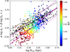 |
Fig. 8. FP for simulated SDGs calculated with the parameters estimated for the ATLAS3D sample. E-SDGs are also depicted according to their B/T ratio. The one-to-one relation (black line) and the best fit for the E-SDGs (magenta line), together with their corresponding rms (dashed lines), are also included for comparison. See Appendix B for the non-smoothed distribution. |
4. Shape and kinematics
In this section, we focus on the core aspect of our study: the intrinsic properties of the E-SDGs and their history of assembly. In order to analyse the relation between shape and kinematics, we calculated the V/σL ratio where V is the average rotational velocity of the SPs and σL is the one dimensional velocity dispersion, within the  . We assume the velocity dispersion to be isotropic in order to derive σL from the 3D σ. The ratio V/σL provides a measure of the relative importance of ordered rotation with respect to velocity dispersion (e.g. Dubois et al. 2016). For the analysed E-SDGs, a maximum V/σL estimated is ∼1.1 whereas a maximum V/σL obtained considering the whole sample (i.e. E-SDGs and E-DDGs) is V/σL ∼ 2.4.
The shape of the E-SDGs are determined by fitting ellipsoides to the 3D stellar distributions (as described in Tissera et al. 2010). For each galaxy, we estimated the semi-axis of the ellipsoides as a ≥ b ≥ c within  . The ellipticity is hereafter defined as
  . Hence, values of ε close to 0 refer to galaxies that are more oblate3.
In Fig. 9, we show the V/σL versus ε. The observed galaxies from ATLAS3D (Emsellem et al. 2011) and the simulated ones are located in similar regions of this plane. From Fig. 9, we can see that the galaxies with the oldest SPs tend to be less oblate and massive. This trend is in global agreement with the results reported by van de Sande et al. (2018). We also find some massive E-SDGs with high V/σL and old SPs in agreement with Lagos et al. (2018) and Cappellari (2016). As can be seen in the bottom panel of this figure, galaxies with high values of B/T tend to have low V/σL. Therefore, hereafter and motivated by this trend, we will define as slow rotators those galaxies with B/T > 0.7 and the rest will be considered fast rotators.
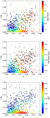 |
Fig. 9. Anisotropy diagram for the E-SDGs. E-SDGs are coloured according to mass-weighted average age (top panel), stellar mass (middle panel) and B/T ratio (bottom panel). Observational data from ATLAS3D are also shown (Emsellem et al. 2011, black crosses). See Appendix B for the non-smoothed distributions. |
5. Mass-growth histories
We investigate the global and radial archaeological MGHs of the E-SDGs. The MGHs were constructed by using the age distributions of the stellar particles at z ∼ 0. We note that because of our selection criteria of the dynamical components, the stellar haloes are not included in our calculations. Three radial bins are defined [0, 0.5], [0.5, 1] and [1, 1.5] of the  , following the observational study of MaNGA galaxies by Ibarra-Medel et al. (2016). We estimated the MGH of each of the 508 E-SDGs.
For this analysis, the E-SDGs are divided in six subsamples. First, we distinguished them according to their stellar masses, defining three subsamples with similar number of galaxies (∼33% of the total in each one). The mass ranges of the subsamples are given in Table 1. Within each mass subsample, B/T, ratios are used to group them according to their morphology: 0.5 < B/T < 0.7 (hereafter, fast rotators) and B/T > 0.7 (hereafter, slow rotators) consistently with Fig. 9 (bottom panel).
Average stacked T70 (Gyr) for SPs in each radial bin for galaxies grouped according to their stellar masses MStar (in units of M⊙).
We calculated the average global and radial MGHs for each group as done in Rosito et al. (2018). These averaged MGHs are normalised to the total mass in each bin (M0) at a lookback time of 0.5 Gyr in order to have a better comparison with observations (Ibarra-Medel et al. 2016). They are shown in Fig. 10. As can be seen from this figure, massive galaxies (upper panels) show very similar MGHs for each radial interval, implying a coeval formation history, on average. However, there is a slight trend for the stars in the inner radial bin to be slightly younger. The MGHs of massive galaxies are in agreement with results by Ibarra-Medel et al. (2016). In order to quantify these trends, we defined the lookback time T70 at which 70% of the stellar mass is already formed. We calculated T70 for each individual galaxy and, in order to understand the global trends, we estimated an average T70 under two different interpretations. On one hand, and for consistency with Rosito et al. (2018) we consider the lookback time at which the average (stacked) MGH for each radial bin reaches the value 0.7 (Table 1). On the other hand, we calculated the mean value of T70 of each bin, considering the individual galaxies grouped as mentioned before. By applying a bootstrap method, we estimated the dispersion of these T70 (Table 2). Both approaches suggest coeval stellar populations for massive galaxies and those with B/T > 0.7.
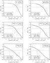 |
Fig. 10. Average global and radial normalised MGH for the E-SDGs: massive galaxies (top panels), intermediate mass galaxies (middle panels), and low mass galaxies (lower panels). Each group is subdivided according to the B/T ratio: fast rotators (left panels) and slow rotators (right panels). The red arrows point out the lookback time at which 70% of the stellar mass in the inner bin is attained. |
Mean T70 (Gyr) values for SPs in each radial bin for galaxies grouped according to their stellar masses MStar (in units of M⊙).
For less massive galaxies, the signals for an overall outside-in formation become stronger. If we consider the stacked T70 as in Table 1, the outside-in trend is present regardless the B/T ratio. By analysing Table 2, we cannot ensure this behaviour within the bootstrap errors for galaxies with high B/T ratios. However, it must be noticed that there are few galaxies with B/T > 0.7 and the dispersion is quite large. In spite of this, we find that T70 moves systematically to earlier values with smaller distances.
The younger populations identified in the central regions could be associated to secular evolution or/and wet minor merger of smaller systems. The MGHs of galaxies with MStar < 1010.46 M⊙ show features (i.e. bumps) that indicates important sudden contributions of SF which might be due to processes such as mergers or gas inflows.
The outside-in formation trends are at odds with the results by Ibarra-Medel et al. (2016) for small stellar mass galaxies4. We note, however, that there are larger uncertainties in the observational determination of ages. This is particularly important for SPs older than ∼7 Gyr. Previous results by Rosito et al. (2018), using galaxies selected from Fenix project (Pedrosa & Tissera 2015), show an overall inside-out formation for SDGs in agreement with the results of Ibarra-Medel et al. (2016). However, we note that our sample of E-SGDs are significantly older, in general, that those observed in recent works, in agreement with van de Sande et al. (2019) where simulations, including EAGLE, are confronted with observations. The youngest galaxy, considering E-SDGs and E-DDGs has a mass-weighted average age of ∼3 Gyr.
Our findings suggest the existence of discs, particularly, in low-mass E-SDGs. These discs could have formed as a results of low efficient transformation of gas into stars at higher redshift that could have left a gas reservoir for late disc formation. The available gas could set on disc structures and feed new SF in the central region via secular evolution. Mergers could also bring in gas that trigger new SF activity. In that case, we expect the younger stars that rejuvenate the central regions of E-SDGs to be associated to the disc components.
To test this, the MGHs for the bulge and disc components are estimated separately as shown in Fig. 11. As bulges are smaller, we considered only two radial bins whereas for the disc components, we use the same bins mentioned above.
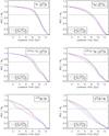 |
Fig. 11. Radial MGHs for both the bulge (red lines) and the disc (blue lines) components of the E-SDGs: massive galaxies (top panels), intermediate mass galaxies (middle panels), and low mass galaxies (lower panels). Each group is subdivided according to the B/T ratio: fast rotators (left panels) and slow rotators (right panels). |
As shown in Table 2, we calculated the values of T70 from which it can be appreciated that discs tend to be younger than bulges (Table 3). For bulges and discs, the SPs are younger for lower mass galaxies as expected. As can be seen from Fig. 11, regardless of mass or B/T ratios, the inner regions of the disc components of the E-SDG are younger, on average. Our results agree with recent findings by Trayford et al. (2019) who show that there is SF activity associated to the disc components in ETGs in the EAGLE simulations. We go further in this analysis and identify that this SF activity is located mainly in the central regions contributing to rejuvenate the SP and to determine an outside-in formation history of the E-SDGs. We note that E-SDGs with younger SPs tend to have B/T < 0.7 and that there is a large spread in the averaged ages, which is due to large variety of MGHs.
Mean T70 (Gyr) values for SPs for bulge and disc components in each radial bin for galaxies grouped according to their stellar masses MStar (in units of M⊙).
The complexity of the formation processes of spheroidal galaxies is reflected in the diversity of features and assembly histories (see e.g. Brooks & Christensen 2016; Kormendy 2016, for recent reviews). To illustrate this, Fig. 12 shows the MGHs of two typical E-SDGs with an inside-out (left panel) and an outside-in (right panel) growth. These two galaxies have similar B/T ratios but the first one is more massive (i.e. MStar ∼ 8.2 × 10¹⁰ M⊙ and MStar ∼ 4.5 × 10¹⁰ M⊙, respectively). The galaxy that formed outside-in shows a larger inner disc fraction (∼0.15 for the outside-in and ∼0.07 for the inside-out galaxy). In general, galaxies with an outside-in behaviour tend to have slightly larger inner discs fractions: the first and third quartiles of these fractions are 0.11 and 0.18 respectively, whereas the corresponding ones for inside-out galaxies are 0.11 and 0.15, respectively. Both MGHs show signature of strong starbursts (i.e. sudden changes in the stellar mass in the MGHs). From this figure, we can also see that bumps are present at all defined radial intervals, suggesting that mergers could be a channel of gas fuelling since they can affect the inner and the outer parts of galaxies by inducing bars and/or accreting material from the incoming systems (Sillero et al. 2017). In Fig. 13, we show the SFR as a function of the look back time for the inside-out galaxy (left panel) and the outside-in one (right panel). It can be seen that in the first one, the main starburst is placed in the inner region at high redshift, whereas in the one with outside-in behaviour, the central region is formed at later epochs. We must be aware that we are studying archaeological MGHs, as done in observations, and we therefore cannot determine only by this analysis whether stars were formed in-situ or they were accreted from satellites (see Trayford et al. 2019, for an ex-situ and in-situ discussion).
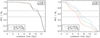 |
Fig. 12. MGHs for two E-SDGs showing different assembly histories: an inside-out (left panel) and an outside-in (right panel). These E-SDGs have similar B/T ratios. |
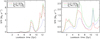 |
Fig. 13. SFR for two E-SDGs showing different assembly histories: an inside-out (left panel) and an outside-in (right panel). These E-SDGs have similar B/T ratios. |
The exploration of the merger trees shows that both have the last mergers event at about 8 − 8.5 Gyr ago but the galaxy with the outside-in formation had a massive merger (1:4) while the galaxy with the inside-out formation had a minor merger (1:10). McAlpine et al. (2018) show that, in the EAGLE simulations massive mergers are efficient mechanisms to trigger the rapidly growth of the central black hole and the triggering of AGN feedback. This result is also reported in previous numerical works (e.g. Springel et al. 2005; Hopkins et al. 2005; Hopkins & Quataert 2010; Capelo et al. 2015). The outside-in formation that we detect some of the E-SDGs, particularly for low mass galaxies might suggest that the SN feedback is not efficient enough to quench the SF and/or that AGN feedback might be needed even in galaxies of about 1010 M⊙ (Argudo-Fernández et al. 2018). Moreover, Manzano-King et al. (2019) provide new observational evidence of AGN activity that would quench SF in low mass galaxies. This is a controversial area of active discussion. In fact previous numerical works suggest that this activity is mainly suppressed by SN feedback in this kind of galaxies (Dubois et al. 2015; Habouzit et al. 2017; Bower et al. 2017; Anglés-Alcázar et al. 2017).
5.1. Bulge and disc global properties
To gain more insight in the assembly process, we explore the global properties, ages and SF efficiency of the bulge and disc components of these galaxies separately. In Fig. 14 we show the mean stellar ages for the spheroid and the disc components in E-SDGs. As can be seen, the bulge and the disc have similar median ages. For both of them there is a correlation with stellar mass so that the more massive galaxies are dominated by the older SPs (conversely, the DDGs show a clear age difference between the bulge and the discs, so that the SPs in the bulges are systematically older by at least 1.5−2 Gyr in comparison to those of the discs, Fig. A.1 as shown in the appendix).
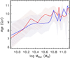 |
Fig. 14. Median stellar ages for bulge (red lines) and disc (blue lines) components as a function of galaxy stellar mass for E-SDGs. The shaded regions represent the first and third quartiles. |
The SF efficiency of the bulge and the disc components show similar trends with galaxy mass as shown in Fig. 15, although the disc components show systematically larger sSFR as expected. Smaller galaxies have slightly stronger SF activity. These global trends over the whole disc and bulge components are in agreement with the analysis of the MGHs.
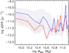 |
Fig. 15. Median sSFR for the bulge (red line) and the disc (blue line) as a function of galaxy stellar mass for the E-SDGs. Shaded regions depict the first and third quartiles. |
5.2. Chemical abundances
Our analysis indicated that the outside-in behaviour is triggered by stars that are formed in the inner region at later time. If these stars are created from enriched gas by earlier SPs, then they could have different chemical abundances. Hence, we investigate their chemical abundances at different radial distances and in relation with their ages. In Fig. 16, the distribution of the median [O/Fe] and median [Fe/H] for the SPs of the E-SDGs as a function of median age of their SPs are shown.
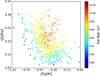 |
Fig. 16. Distribution of median [O/Fe] and median [Fe/H] for the E-SDGs coloured according to median ages of the total SPs. See Appendix B for the non-smoothed distribution. |
The median abundances for each E-SDGs are estimated by using the individual values for each single SP (i.e. represented by a star particle) within the  . Hence, the SPs in the very outer regions are not included.
Overall, stars in the E-SDGs are α-enhanced as expected. The [O/Fe] decreases with increasing [Fe/H]. As can be seen from this figure, massive galaxies dominated by old stars have [Fe/H] in the range [ − 0.6, −0.2] dex and are α-enriched (see also Vincenzo et al. 2018). This is consistent with the fact that more massive galaxies tend to form stars in strong starbursts that also quenched the subsequent SF (via stellar or AGN feedback). E-SDGs with younger stars are distributed in a type of U-shape: those with higher [O/Fe] are located at low metallicities while poor-α systems move to higher metallicities. These trends are consistent with a larger variety in assembly histories for smaller galaxies and SF activity (with more than one burst).
In Fig. 17 we show the distributions of [O/Fe] and [Fe/H] calculated within each radial bin considered in Fig. 10. There is a slight trend for lower [O/Fe] at low [Fe/H] for SPs in the inner radial bin. This suggests that a fraction of the inner stars formed from pre-enriched material compared to the outer parts. From this plot, we can also see that the outer radial regions have a larger contribution of old and α-rich stars. These behaviours could be explained by the later accretion of gas into the central regions via secular evolution and/or the contribution of old, high α-enriched stars acquired by accretion of small satellites (Clauwens et al. 2018). We acknowledge the fact that there is a large dispersion in the abundance relations that prevents a robust conclusion. This analysis is intended to provide a description of the chemical abundance distributions which can serve as basis for future improvements.
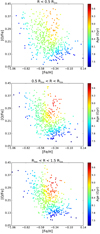 |
Fig. 17. Distribution of median [O/Fe] and median [Fe/H] within each radial bin. Symbols are coloured according to mean ages. See Appendix B for the non-smoothed distribution. |
6. Conclusions
We have performed a comprehensive study of a sample of well-resolved numerical spheroid dominated galaxies from the EAGLE simulation. The features and behaviours of these systems are confronted with previous results. A galaxy is considered a SDG if B/T > 0.5.
We find the following results:
-
(i)
In agreement with Rosito et al. (2018), all E-SDGs are found to host disc component. Part of these discs co-exists with the bulge. The mass fraction of inner disc over the bulge anti-correlates with B/T ratio.
-
(ii)
Most of E-SDGs have Sérsic indexes n < 2 that increases with B/T ratio in agreement with observations (Fisher & Drory 2008). Furthermore, we find that galaxies with larger B/T ratios are more massive and have older SPs.
-
(iii)
E-SDGs follow scaling relations such as the FJR and FP, in agreement with observations (Cappellari et al. 2013a,b). Regarding the size-mass relation, there is also a reasonable agreement with observations, although E-SDGs with lower B/T ratios tend to be more extended. An exhaustive analysis of the size-mass relation is given by Rosito et al. (2019).
-
(iv)
By analysing the relation between shape and kinematics, we find trend that agree with results by Emsellem et al. (2011), who report that a significant fraction of ETGs tend to be fast rotators. The relations between shape and kinematics indicators are consistent with observations from ATLAS3D. We find a trend for less oblate E-SDGs to have older SPs and to be slower rotators in global agreement with observations. The median stellar ages estimated for the E-SDGs are within the range [3.4, 12.7] Gyr with the median value at ∼8.7 Gyr. These ages are older than reported by observations in agrement with the results found by van de Sande et al. (2019).
-
(v)
The MGHs of the E-SDGs suggest different assembly histories according to the stellar mass of the galaxies in global agreement with the picture described by Clauwens et al. (2018) for the complete sample of EAGLE galaxies. In general, there is a large variety of MGHs for the galaxies analysed in this work and in many of them there are signals of mergers and starbursts. E-SDGs with stellar masses in the range 1010.5 M⊙ < MStar < 1011.2 M⊙ have MGHs consistent with almost coeval SPs, with a slight trend for the inner regions to be ∼0.5 Gyr younger than the outskirts. E-SDGs with B/T > 0.7 are consistent to have coeval SPs that are systematically older than those in systems with B/T < 0.7 in the same mass range. For less massive galaxies, there is an increasing contribution of younger SPs within the 0.5Rhm, that translates into an age gap between the median age of the inner SPs and that of the outer SPs. The age gap increases from ∼0.5 Gyr for the most massive analysed E-SDGs to ∼2 Gyr for the smallest ones. The outside-in assembly of ETGs with MStar < 1010.5 M⊙ is in tension with current observational findings.
-
(vi)
We find that, at a given median [Fe/H], more massive and older E-SDGs have higher [O/Fe] abundances. E-SDGs with MStar < 1010 M⊙ determine a U-shape relation showing a larger variety of chemical abundances in [Fe/H] vs [O/Fe]. The outside-in scenario is consistent with the chemical abundances estimated for SPs at different radial distances. The larger values of [O/Fe] in the outer regions are consistent with stars formed in short starbursts so that the pristine gas could not have been enriched with iron due to SNIa. This trend supports the suggestion that part of the outer stellar enveloped is formed by accreted material (e.g. Clauwens et al. 2018). On the other hand the slightly younger stars with lower [O/Fe] in the inner regions indicates that they might have formed from pre-enriched gas.
-
(vii)
As mentioned before, all selected E-SDGs have a disc component, even if it represents a small fraction of the total mass. The disc concentrates most of the SF activity which is preferentially located in the central regions. This is not the case for those galaxies dominated by discs. We find that E-DDG (i.e. B/T < 0.5) to show a clear ordered MGHs consistent with an inside-out scenario. Hence, galaxies that reach z = 0 as spiral galaxies have managed to grow orderly in an inside-out fashion (see Appendix A). We speculate that the following mechanisms could have played a role at modulating the assembly of ETGs. On one hand, the existence of discs in the E-SDGs makes them more susceptible to the effects of secular evolution that can drive gas inflows and feed SF in the central region. Stronger SN feedback could help to solve this problem. AGN feedback might be also needed to act in smaller galaxies as suggested by recent observational results (Argudo-Fernández et al. 2018; Manzano-King et al. 2019). However, a number of numerical results claimed for less important role of AGN feedback at low mass (e.g. Dubois et al. 2015; Anglés-Alcázar et al. 2017). Hence, this is still a controversial issue in galaxy formation. On the other hand, considering the results of Clauwens et al. (2018) that showed a contribution of ex-situ stars at r > 5 kpc, ranging from 10 to 60 per cent, depending on galaxy mass, it might be possible that the accretion of satellites in the outer regions works to enhance the outside-in formation trend as they would contribute with old stars. These minor mergers could also play a role at destabilising an existing disc component. This is a very interesting aspect to explore in more detail in a future work.
The optical radius, Ropt, is defined as the one that encloses ∼80% of the baryonic mass (gas and stars) of the galaxy (Tissera 2000). This definition allows a determination of a characteristic radius that adapts to the size and mass distribution of a given galaxy.
There is a difference between our definition of stellar mass and the one used in Schaye et al. (2015). In the latter case, the stellar mass is defined as the sum of masses of all star particles within a radius of 30 kpc.
This is the intrinsic ellipticity, which is equivalent to that estimated by Trayford et al. (2019).
In the appendix, we show that DDGs selected from the same simulation have, on average, an inside-out formation (Fig. A.2) as reported by previous work (Zavala et al. 2016; Tissera et al. 2019).
Acknowledgments
PBT acknowledges partial support from Fondecyt 1150334 (Conicyt). The use of RAGNAR cluster funded by Fondecyt 1150334 and UNAB is acknowledged. This project has received funding from the European Union Horizon 2020 Research and Innovation Programme under the Marie Sklodowska-Curie grant agreement No 734374. This work used the DiRAC Data Centric system at Durham University, operated by the Institute for Computational Cosmology on behalf of the STFC DiRAC HPC Facility (www.dirac.ac.uk). This equipment was funded by BIS National E-infrastructure capital grant ST/K00042X/1, STFC capital grants ST/H008519/1 and ST/K00087X/1, STFC DiRAC Operations grant ST/K003267/1 and Durham University. DiRAC is part of the National E-Infrastructure. We acknowledge PRACE for awarding us access to the Curie machine based in France at TGCC, CEA, Bruyeresle-Chatel.
References
- Anglés-Alcázar, D., Faucher-Giguère, C.-A., Quataert, E., et al. 2017, MNRAS, 472, L109 [NASA ADS] [CrossRef] [Google Scholar]
- Argudo-Fernández, M., Lacerna, I., & Duarte Puertas, S. 2018, A&A, 620, A113 [NASA ADS] [CrossRef] [EDP Sciences] [Google Scholar]
- Avila-Reese, V., Zavala, J., & Lacerna, I. 2014, MNRAS, 441, 417 [NASA ADS] [CrossRef] [Google Scholar]
- Bernardi, M., Meert, A., Vikram, V., et al. 2014, MNRAS, 443, 874 [NASA ADS] [CrossRef] [Google Scholar]
- Bournaud, F., Jog, C. J., & Combes, F. 2007, A&A, 476, 1179 [NASA ADS] [CrossRef] [EDP Sciences] [Google Scholar]
- Bower, R. G., Schaye, J., Frenk, C. S., et al. 2017, MNRAS, 465, 32 [NASA ADS] [CrossRef] [Google Scholar]
- Brooks, A., & Christensen, C. 2016, Galact. Bulg., 418, 317 [Google Scholar]
- Bundy, K., Bershady, M. A., Law, D. R., et al. 2015, ApJ, 798, 7 [NASA ADS] [CrossRef] [Google Scholar]
- Burkert, A., & Naab, T. 2004, Coevolution of Black Holes and Galaxies (Cambridge University Press), 421 [Google Scholar]
- Bustamente, S. 2018, Galaxy Interactions and Mergers Across Cosmic Time, held 11–16 March, 2018 in Sexten, Italy, 47 [Google Scholar]
- Capelo, P. R., Volonteri, M., Dotti, M., et al. 2015, MNRAS, 447, 2123 [NASA ADS] [CrossRef] [Google Scholar]
- Cappellari, M. 2016, ARA&A, 54, 597 [NASA ADS] [CrossRef] [Google Scholar]
- Cappellari, M., Emsellem, E., Krajnović, D., et al. 2011, MNRAS, 413, 813 [NASA ADS] [CrossRef] [Google Scholar]
- Cappellari, M., McDermid, R., Alatalo, K., et al. 2013a, MNRAS, 432, 1709 [NASA ADS] [CrossRef] [Google Scholar]
- Cappellari, M., McDermid, R. M., Alatalo, K., et al. 2013b, MNRAS, 432, 1862 [NASA ADS] [CrossRef] [Google Scholar]
- Chabrier, G. 2003, PASP, 115, 763 [NASA ADS] [CrossRef] [Google Scholar]
- Clauwens, B., Schaye, J., Franx, M., & Bower, R. G. 2018, MNRAS, 478, 3994 [NASA ADS] [CrossRef] [Google Scholar]
- Cleveland, W. S., & Devlin, S. J. 1988, J. Am. Stat. Assoc., 83, 596 [CrossRef] [Google Scholar]
- Crain, R. A., Schaye, J., Bower, R. G., et al. 2015, MNRAS, 450, 1937 [NASA ADS] [CrossRef] [Google Scholar]
- Croom, S. M., Lawrence, J. S., Bland-Hawthorn, J., et al. 2012, MNRAS, 421, 872 [NASA ADS] [Google Scholar]
- Dalla Vecchia, C., & Schaye, J. 2012, MNRAS, 426, 140 [NASA ADS] [CrossRef] [Google Scholar]
- De Rossi, M. E., Theuns, T., Font, A. S., & McCarthy, I. G. 2015, MNRAS, 452, 486 [NASA ADS] [CrossRef] [Google Scholar]
- Djorgovski, S., & Davis, M. 1987, ApJ, 313, 59 [NASA ADS] [CrossRef] [Google Scholar]
- Dressler, A., Lynden-Bell, D., Burstein, D., et al. 1987, ApJ, 313, 42 [NASA ADS] [CrossRef] [Google Scholar]
- Dubois, Y., Volonteri, M., Silk, J., et al. 2015, MNRAS, 452, 1502 [NASA ADS] [CrossRef] [Google Scholar]
- Dubois, Y., Peirani, S., Pichon, C., et al. 2016, MNRAS, 463, 3948 [NASA ADS] [CrossRef] [Google Scholar]
- Emsellem, E., Cappellari, M., Krajnović, D., et al. 2011, MNRAS, 414, 888 [NASA ADS] [CrossRef] [Google Scholar]
- Faber, S., & Jackson, R. 1976, ApJ, 204, 668 [NASA ADS] [CrossRef] [Google Scholar]
- Faber, S. M., Dressler, A., Davies, R. L., Burstein, D., & Lynden-Bell, D. 1987, in Nearly Normal Galaxies. From the Planck Time to the Present, ed. S. M. Faber, 175 [Google Scholar]
- Falcón-Barroso, J., & Knapen, J. 2012, Secular Evolution of Galaxies, Canary Islands Winter School of Astrophysics (Cambridge University Press) [Google Scholar]
- Fisher, D. B., & Drory, N. 2008, AJ, 136, 773 [NASA ADS] [CrossRef] [Google Scholar]
- Genel, S., Vogelsberger, M., Springel, V., et al. 2014, MNRAS, 445, 175 [Google Scholar]
- Genel, S., Fall, S. M., Hernquist, L., et al. 2015, ApJ, 804, L40 [NASA ADS] [CrossRef] [Google Scholar]
- Genel, S., Nelson, D., Pillepich, A., et al. 2018, MNRAS, 474, 3976 [NASA ADS] [CrossRef] [Google Scholar]
- Gibson, B. K., Pilkington, K., Brook, C. B., Stinson, G. S., & Bailin, J. 2013, A&A, 554, A47 [NASA ADS] [CrossRef] [EDP Sciences] [Google Scholar]
- González-García, A. C., Oñorbe, J., Domínguez-Tenreiro, R., & Gómez-Flechoso, M. Á. 2009, A&A, 497, 35 [NASA ADS] [CrossRef] [EDP Sciences] [Google Scholar]
- Habouzit, M., Volonteri, M., & Dubois, Y. 2017, MNRAS, 468, 3935 [NASA ADS] [CrossRef] [Google Scholar]
- Hernquist, L. 1989, Nature, 340, 687 [NASA ADS] [CrossRef] [Google Scholar]
- Hopkins, P. F., & Quataert, E. 2010, MNRAS, 407, 1529 [NASA ADS] [CrossRef] [Google Scholar]
- Hopkins, P. F., Hernquist, L., Cox, T. J., et al. 2005, ApJ, 630, 705 [NASA ADS] [CrossRef] [Google Scholar]
- Ibarra-Medel, H. J., Sánchez, S. F., Avila-Reese, V., & Hernández-Toledo, H. M. 2016, MNRAS, 463, 2799 [NASA ADS] [CrossRef] [Google Scholar]
- Kormendy, J. 2016, Galact. Bulg., 418, 431 [NASA ADS] [CrossRef] [Google Scholar]
- Lagos, C. D. P., Schaye, J., Bahé, Y., et al. 2018, MNRAS, 476, 4327 [NASA ADS] [CrossRef] [Google Scholar]
- Li, C., Wang, E., Lin, L., et al. 2015, ApJ, 804, 125 [NASA ADS] [CrossRef] [Google Scholar]
- Lin, L., Zou, H., Kong, X., et al. 2013, ApJ, 769, 127 [NASA ADS] [CrossRef] [Google Scholar]
- Manzano-King, C., Canalizo, G., & Sales, L. 2019, ArXiv e-prints [arXiv:1905.09287] [Google Scholar]
- McAlpine, S., Helly, J. C., Schaller, M., et al. 2016, Astron. Comput., 15, 72 [NASA ADS] [CrossRef] [Google Scholar]
- McAlpine, S., Bower, R. G., Rosario, D. J., et al. 2018, MNRAS, 481, 3118 [NASA ADS] [CrossRef] [Google Scholar]
- Mihos, J. C., & Hernquist, L. 1996, ApJ, 464, 641 [NASA ADS] [CrossRef] [Google Scholar]
- Mosleh, M., Williams, R. J., & Franx, M. 2013, ApJ, 777, 117 [NASA ADS] [CrossRef] [Google Scholar]
- Naab, T. 2013, in The Intriguing Life of Massive Galaxies, eds. D. Thomas, A. Pasquali, & I. Ferreras, IAU Symp., 295, 340 [NASA ADS] [Google Scholar]
- Pedrosa, S. E., & Tissera, P. B. 2015, A&A, 584, A43 [NASA ADS] [CrossRef] [EDP Sciences] [Google Scholar]
- Perez, J., Valenzuela, O., Tissera, P. B., & Michel-Dansac, L. 2013, MNRAS, 436, 259 [NASA ADS] [CrossRef] [Google Scholar]
- Planck Collaboration I. 2014, A&A, 571, A1 [NASA ADS] [CrossRef] [EDP Sciences] [Google Scholar]
- Planck Collaboration XVI. 2014, A&A, 571, A16 [NASA ADS] [CrossRef] [EDP Sciences] [Google Scholar]
- Rodriguez-Gomez, V., Genel, S., Vogelsberger, M., et al. 2015, MNRAS, 449, 49 [NASA ADS] [CrossRef] [Google Scholar]
- Rodriguez-Gomez, V., Pillepich, A., Sales, L. V., et al. 2016, MNRAS, 458, 2371 [NASA ADS] [CrossRef] [Google Scholar]
- Rosas-Guevara, Y. M., Bower, R. G., Schaye, J., et al. 2015, MNRAS, 454, 1038 [CrossRef] [Google Scholar]
- Rosito, M. S., Pedrosa, S. E., Tissera, P. B., et al. 2018, A&A, 614, A85 [NASA ADS] [CrossRef] [EDP Sciences] [Google Scholar]
- Rosito, M. S., Tissera, P., Pedrosa, S. & Lagos, C. 2019, A&A, 629, L3 [CrossRef] [EDP Sciences] [Google Scholar]
- Rupke, D. S. N., Kewley, L. J., & Barnes, J. E. 2010, ApJ, 710, L156 [NASA ADS] [CrossRef] [Google Scholar]
- Sáiz, A., Domínguez-Tenreiro, R., Tissera, P. B., & Courteau, S. 2001, MNRAS, 325, 119 [NASA ADS] [CrossRef] [Google Scholar]
- Salpeter, E. E. 1955, ApJ, 121, 161 [Google Scholar]
- Sánchez, S. F., Kennicutt, R. C., Gil de Paz, A., et al. 2012, A&A, 538, A8 [NASA ADS] [CrossRef] [EDP Sciences] [Google Scholar]
- Sánchez-Blázquez, P., Forbes, D. A., Strader, J., Brodie, J., & Proctor, R. 2007, MNRAS, 377, 759 [NASA ADS] [CrossRef] [Google Scholar]
- Schaye, J., & Dalla Vecchia, C. 2008, MNRAS, 383, 1210 [NASA ADS] [CrossRef] [EDP Sciences] [Google Scholar]
- Schaye, J., Crain, R. A., Bower, R. G., et al. 2015, MNRAS, 446, 521 [Google Scholar]
- SDSS Collaboration (Albareti, F. D., et al.) 2017, ApJS, 233, 25 [NASA ADS] [CrossRef] [Google Scholar]
- Sérsic, J. L. 1968, Atlas de Galaxias Australes (Cordoba, Argentina: Observatorio Astronomico) [Google Scholar]
- Sillero, E., Tissera, P. B., Lambas, D. G., & Michel-Dansac, L. 2017, MNRAS, 472, 4404 [NASA ADS] [CrossRef] [Google Scholar]
- Springel, V., Di Matteo, T., & Hernquist, L. 2005, MNRAS, 361, 776 [NASA ADS] [CrossRef] [Google Scholar]
- Taylor, P., & Kobayashi, C. 2017, MNRAS, 471, 3856 [NASA ADS] [CrossRef] [Google Scholar]
- Tissera, P. B. 2000, ApJ, 534, 636 [NASA ADS] [CrossRef] [Google Scholar]
- Tissera, P. B. 2012, Boletin de la Asociacion Argentina de Astronomia La Plata Argentina, 55, 233 [NASA ADS] [Google Scholar]
- Tissera, P. B., White, S. D. M., Pedrosa, S., & Scannapieco, C. 2010, MNRAS, 406, 922 [NASA ADS] [Google Scholar]
- Tissera, P. B., White, S. D. M., & Scannapieco, C. 2012, MNRAS, 420, 255 [NASA ADS] [CrossRef] [Google Scholar]
- Tissera, P. B., Machado, R. E. G., Sanchez-Blazquez, P., et al. 2016, A&A, 592, A93 [NASA ADS] [CrossRef] [EDP Sciences] [Google Scholar]
- Tissera, P. B., Rosas-Guevara, Y., Bower, R. G., et al. 2019, MNRAS, 482, 2208 [NASA ADS] [CrossRef] [Google Scholar]
- Trayford, J. W., Frenk, C. S., Theuns, T., Schaye, J., & Correa, C. 2019, MNRAS, 483, 744 [NASA ADS] [CrossRef] [Google Scholar]
- van de Sande, J., Scott, N., Bland-Hawthorn, J., et al. 2018, Nat. Astron., 2, 483 [NASA ADS] [CrossRef] [Google Scholar]
- van de Sande, J., Lagos, C. D. P., Welker, C., et al. 2019, MNRAS, 484, 869 [NASA ADS] [CrossRef] [Google Scholar]
- Vincenzo, F., Kobayashi, C., & Taylor, P. 2018, MNRAS, 480, L38 [NASA ADS] [Google Scholar]
- Vogelsberger, M., Genel, S., Springel, V., et al. 2014a, Nature, 509, 177 [NASA ADS] [CrossRef] [Google Scholar]
- Vogelsberger, M., Genel, S., Springel, V., et al. 2014b, MNRAS, 444, 1518 [NASA ADS] [CrossRef] [Google Scholar]
- Wang, J., Kauffmann, G., Overzier, R., et al. 2011, MNRAS, 412, 1081 [Google Scholar]
- Wiersma, R. P. C., Schaye, J., & Smith, B. D. 2009, MNRAS, 393, 99 [NASA ADS] [CrossRef] [Google Scholar]
- Zavala, J., Avila-Reese, V., Firmani, C., & Boylan-Kolchin, M. 2012, MNRAS, 427, 1503 [NASA ADS] [CrossRef] [Google Scholar]
- Zavala, J., Frenk, C. S., Bower, R., et al. 2016, MNRAS, 460, 4466 [NASA ADS] [CrossRef] [Google Scholar]
Appendix A: Comparison with the disc-dominated galaxies
For comparison purposes, we also analyse some of the relations studied in the main section for all galaxies resolved with more than 10 000 particles. This sample comprises 70% of E-DDGs and 30% of E-SDGs.
In Sect. 5, we emphasise the fact that SDGs in the EAGLE simulation tend to show an outside-in growth. However as expected this is not the case for DDGs. The inside-out scenario is consistent with previous analysis of the EAGLE simulations (Zavala et al. 2016; Tissera et al. 2019). While no significant differences between the mean ages of the bulge and disc components of E-SDGs are found (Sect. 5), in the DDGs bulges are older than discs by about ∼2 Gyr (Fig. A.1). The average global and radial MGHs for DDGs can be seen in Fig. A.2. The 70% of the stellar mass in the inner, intermediate and outer radial intervals is attained at lookback times of 6.5 Gyr, 6 Gyr and 5.5 Gyr, respectively.
 |
Fig. A.1. Median stellar ages for the bulge (red lines) and disc (blue lines) components as a function of galaxy stellar mass for DDGs. The shadowed regions represent the first and third quartiles. |
 |
Fig. A.2. Average global and radial normalised MGH for the DDGs. It presents a clear inside-out growth. |
In Sect. 5 we find the sSFR of disc and bulge components of E-SDGs are similar. However, when all galaxies in the sample regardless of the B/T ratios are considered a trend for higher B/T ratio to have the lower sSFR as shown in Fig. A.3.
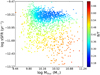 |
Fig. A.3. sSFR as a function of stellar mass of the total analysed sample. Symbols are coloured according to the B/T ratio. See Appendix B for the non-smoothed distribution. |
We remark that in these plots we did not fix the colour-bar limits to the first and third quartiles of the variable according to which we colour the symbols. Instead we use a wider range. The reason for this is that most of the galaxies in our sample are DDGs, and therefore have B/T lower than 0.5.
Appendix B: Non-smoothed distributions
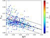 |
Fig. B.1. Stellar-mass fractions Frot of the discs that co-exist with the spheroidal components as a function of the B/T ratio. Symbols are coloured according to n. A linear regression fit is included (solid black line) along with its 1σ dispersion (dashed black lines). In this figure, we do not fix the colour-bar limits. |
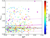 |
Fig. B.2. Sérsic index (nSersic) as a function of B/T ratio for the simulated E-SDGs, coloured according to the mass-weighted average age of the galaxy stellar mass. A linear regression fit is included (solid magenta line) with its 1σ dispersion (dashed magenta line). For comparison, we also include the results by Rosito et al. (2018; magenta squares). The line nSersic = 1 is depicted in a black line. |
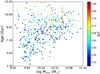 |
Fig. B.3. Mass-weighted average stellar age of the E-SDGs (i.e. bulge and disc SPs) as a function of stellar mass for the simulated galaxies. The symbols are coloured according to the B/T ratios. |
In this appendix we show the scatter plots of the figures analysed in Sects. 4 and 5 without applying the smoothing method of Cappellari et al. (2013b) in order to provide a mean to assess the real distributions.
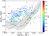 |
Fig. B.4. Mass-size relation estimated for the E-SDGs. Symbols are coloured according to their B/T ratio. The median of the observations from ATLAS3D (black line; the first and third quartiles are shown as shadowed region) and the observed relations for ETGs reported by Mosleh et al. (2013, solid magenta line) and Bernardi et al. (2014, dashed blue line) are included for comparison. |
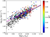 |
Fig. B.5. FJR for simulated E-SDGs (filled circles) and observed ETGs from ATLAS3D (black crosses) galaxies. The least squared regression lines are included in magenta and black line for simulated and observed data, respectively. |
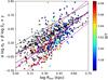 |
Fig. B.6. FP for the simulated SDGs calculated with the parameters estimated for the ATLAS3D sample. E-SDGs are also depicted according to their B/T ratio. The black line denotes the one-to-one relation and the magenta line represents the best fit for the E-SDGs. In dashed lines we show the rms corresponding to the least squared regression and the one-to-one relation. |
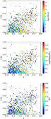 |
Fig. B.7. Anisotropy diagram for the E-SDGs. E-SDGs are coloured according to mass-weighted average age (top panel), stellar mass (middle panel) and B/T ratio (bottom panel). Observational data from ATLAS3D are also shown (Emsellem et al. 2011, black crosses). |
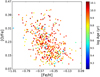 |
Fig. B.8. Distribution of [O/Fe] and [Fe/H] for the E-SDGs coloured according to the median ages of the total SPs. |
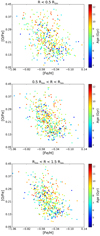 |
Fig. B.9. Distribution of [O/Fe] and [Fe/H] within each radial bin. Symbols are coloured according to mean ages. |
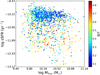 |
Fig. B.10. sSFR as a function of stellar mass of the total analysed sample. Symbols are coloured according to B/T ratio. |
All Tables
Average stacked T70 (Gyr) for SPs in each radial bin for galaxies grouped according to their stellar masses MStar (in units of M⊙).
Mean T70 (Gyr) values for SPs in each radial bin for galaxies grouped according to their stellar masses MStar (in units of M⊙).
Mean T70 (Gyr) values for SPs for bulge and disc components in each radial bin for galaxies grouped according to their stellar masses MStar (in units of M⊙).
All Figures
|
Fig. 1. Distribution of B/T ratios for selected EAGLE galaxies. Only those galaxies with B/T > 0.5 are classified as SDGs (dashed magenta line). |
| In the text | |
|
Fig. 2. Projected stellar-mass surface density profiles for bulge (red diamonds) and disc components (blue diamonds) of two typical simulated ETGs. The regions of the discs that co-exist with spheroid components are highlighted (green diamonds). The best-fitted Sérsic profiles for the spheroid components (solid red lines) and the exponential profiles for the discs (dashed blue lines) are also included. The bulge effective radius (Reff, calculated by using Eq. (6) in Sáiz et al. 2001), the Rhm and the Rd are depicted with red, black and blue arrows, respectively. In the upper panel, the inner disc follows the exponential profile (n ∼ 1.25) while in the lower panel, the same component follows the bulge profile (n ∼ 2.78). A variety of behaviours is detected, suggesting different contributions of processes such as collapse, mergers and secular evolution. |
| In the text | |
|
Fig. 3. Stellar-mass fractions Frot of the discs that co-exist with the spheroidal components as a function of the B/T ratio. Symbols are coloured according to n. A linear regression fit is included (solid black line) along with its 1σ dispersion (dashed black lines). |
| In the text | |
|
Fig. 4. Sérsic index (nSersic) as a function of B/T ratio for the simulated E-SDGs, coloured according to the mass-weighted average age of the galaxy stellar mass. A linear regression fit is included (solid magenta line) with its 1σ dispersion (dashed magenta line). For comparison, we also include the results by Rosito et al. (2018; magenta squares). The line nSersic = 1 is depicted in a black line. See Appendix B for the non-smoothed distribution. |
| In the text | |
|
Fig. 5. Mass-weighted stellar age of the E-SDGs (i.e. bulge and disc SPs) as a function of stellar mass for the simulated galaxies. The symbols are coloured according to the B/T ratios. See Appendix B for the non-smoothed distribution. |
| In the text | |
|
Fig. 6. Mass-size relation estimated for E-SDGs. Symbols are coloured according to their B/T ratio. The medians of the observations from ATLAS3D (black line; the first and third quartiles are shown as shadowed region) and the observed relations for ETGs reported by Mosleh et al. (2013, solid magenta line) and Bernardi et al. (2014, dashed blue line) are included for comparison. See Appendix B for the non-smoothed distribution. |
| In the text | |
|
Fig. 7. FJR for simulated E-SDGs (filled circles) and observed ETGs from ATLAS3D (black crosses) galaxies. The symbols are coloured according to their B/T ratios. The least squared regressions are included for simulated and observed data (magenta and black lines, respectively). See Appendix B for the non-smoothed distributions. |
| In the text | |
|
Fig. 8. FP for simulated SDGs calculated with the parameters estimated for the ATLAS3D sample. E-SDGs are also depicted according to their B/T ratio. The one-to-one relation (black line) and the best fit for the E-SDGs (magenta line), together with their corresponding rms (dashed lines), are also included for comparison. See Appendix B for the non-smoothed distribution. |
| In the text | |
|
Fig. 9. Anisotropy diagram for the E-SDGs. E-SDGs are coloured according to mass-weighted average age (top panel), stellar mass (middle panel) and B/T ratio (bottom panel). Observational data from ATLAS3D are also shown (Emsellem et al. 2011, black crosses). See Appendix B for the non-smoothed distributions. |
| In the text | |
|
Fig. 10. Average global and radial normalised MGH for the E-SDGs: massive galaxies (top panels), intermediate mass galaxies (middle panels), and low mass galaxies (lower panels). Each group is subdivided according to the B/T ratio: fast rotators (left panels) and slow rotators (right panels). The red arrows point out the lookback time at which 70% of the stellar mass in the inner bin is attained. |
| In the text | |
|
Fig. 11. Radial MGHs for both the bulge (red lines) and the disc (blue lines) components of the E-SDGs: massive galaxies (top panels), intermediate mass galaxies (middle panels), and low mass galaxies (lower panels). Each group is subdivided according to the B/T ratio: fast rotators (left panels) and slow rotators (right panels). |
| In the text | |
|
Fig. 12. MGHs for two E-SDGs showing different assembly histories: an inside-out (left panel) and an outside-in (right panel). These E-SDGs have similar B/T ratios. |
| In the text | |
|
Fig. 13. SFR for two E-SDGs showing different assembly histories: an inside-out (left panel) and an outside-in (right panel). These E-SDGs have similar B/T ratios. |
| In the text | |
|
Fig. 14. Median stellar ages for bulge (red lines) and disc (blue lines) components as a function of galaxy stellar mass for E-SDGs. The shaded regions represent the first and third quartiles. |
| In the text | |
|
Fig. 15. Median sSFR for the bulge (red line) and the disc (blue line) as a function of galaxy stellar mass for the E-SDGs. Shaded regions depict the first and third quartiles. |
| In the text | |
|
Fig. 16. Distribution of median [O/Fe] and median [Fe/H] for the E-SDGs coloured according to median ages of the total SPs. See Appendix B for the non-smoothed distribution. |
| In the text | |
|
Fig. 17. Distribution of median [O/Fe] and median [Fe/H] within each radial bin. Symbols are coloured according to mean ages. See Appendix B for the non-smoothed distribution. |
| In the text | |
|
Fig. A.1. Median stellar ages for the bulge (red lines) and disc (blue lines) components as a function of galaxy stellar mass for DDGs. The shadowed regions represent the first and third quartiles. |
| In the text | |
|
Fig. A.2. Average global and radial normalised MGH for the DDGs. It presents a clear inside-out growth. |
| In the text | |
|
Fig. A.3. sSFR as a function of stellar mass of the total analysed sample. Symbols are coloured according to the B/T ratio. See Appendix B for the non-smoothed distribution. |
| In the text | |
|
Fig. B.1. Stellar-mass fractions Frot of the discs that co-exist with the spheroidal components as a function of the B/T ratio. Symbols are coloured according to n. A linear regression fit is included (solid black line) along with its 1σ dispersion (dashed black lines). In this figure, we do not fix the colour-bar limits. |
| In the text | |
|
Fig. B.2. Sérsic index (nSersic) as a function of B/T ratio for the simulated E-SDGs, coloured according to the mass-weighted average age of the galaxy stellar mass. A linear regression fit is included (solid magenta line) with its 1σ dispersion (dashed magenta line). For comparison, we also include the results by Rosito et al. (2018; magenta squares). The line nSersic = 1 is depicted in a black line. |
| In the text | |
|
Fig. B.3. Mass-weighted average stellar age of the E-SDGs (i.e. bulge and disc SPs) as a function of stellar mass for the simulated galaxies. The symbols are coloured according to the B/T ratios. |
| In the text | |
|
Fig. B.4. Mass-size relation estimated for the E-SDGs. Symbols are coloured according to their B/T ratio. The median of the observations from ATLAS3D (black line; the first and third quartiles are shown as shadowed region) and the observed relations for ETGs reported by Mosleh et al. (2013, solid magenta line) and Bernardi et al. (2014, dashed blue line) are included for comparison. |
| In the text | |
|
Fig. B.5. FJR for simulated E-SDGs (filled circles) and observed ETGs from ATLAS3D (black crosses) galaxies. The least squared regression lines are included in magenta and black line for simulated and observed data, respectively. |
| In the text | |
|
Fig. B.6. FP for the simulated SDGs calculated with the parameters estimated for the ATLAS3D sample. E-SDGs are also depicted according to their B/T ratio. The black line denotes the one-to-one relation and the magenta line represents the best fit for the E-SDGs. In dashed lines we show the rms corresponding to the least squared regression and the one-to-one relation. |
| In the text | |
|
Fig. B.7. Anisotropy diagram for the E-SDGs. E-SDGs are coloured according to mass-weighted average age (top panel), stellar mass (middle panel) and B/T ratio (bottom panel). Observational data from ATLAS3D are also shown (Emsellem et al. 2011, black crosses). |
| In the text | |
|
Fig. B.8. Distribution of [O/Fe] and [Fe/H] for the E-SDGs coloured according to the median ages of the total SPs. |
| In the text | |
|
Fig. B.9. Distribution of [O/Fe] and [Fe/H] within each radial bin. Symbols are coloured according to mean ages. |
| In the text | |
|
Fig. B.10. sSFR as a function of stellar mass of the total analysed sample. Symbols are coloured according to B/T ratio. |
| In the text | |
Current usage metrics show cumulative count of Article Views (full-text article views including HTML views, PDF and ePub downloads, according to the available data) and Abstracts Views on Vision4Press platform.
Data correspond to usage on the plateform after 2015. The current usage metrics is available 48-96 hours after online publication and is updated daily on week days.
Initial download of the metrics may take a while.