| Issue |
A&A
Volume 628, August 2019
|
|
|---|---|---|
| Article Number | A48 | |
| Number of page(s) | 10 | |
| Section | Planets and planetary systems | |
| DOI | https://doi.org/10.1051/0004-6361/201935868 | |
| Published online | 06 August 2019 | |
Disintegration of active asteroid P/2016 G1 (PANSTARRS)
1
European Southern Observatory,
Karl-Schwarzschild-Strasse 2,
85748
Garching bei München,
Germany
e-mail: This email address is being protected from spambots. You need JavaScript enabled to view it.
2
Institute for Astronomy,
2680 Woodlawn Drive,
Honolulu,
HI
96822,
USA
3
University of NM – 1700 Lomas Blvd,
NE. Suite 2200,
Albuquerque,
NM
87131-0001
USA
4
ESA SSA-NEO Coordination Centre,
Largo Galileo Galilei,
1 00044
Frascati
(RM),
Italy
5
INAF – Osservatorio Astronomico di Roma,
Via Frascati, 33,
00040
Monte Porzio Catone
(RM),
Italy
6
Indian Institute of Astrophysics,
II Block, Koramangala,
Bengaluru
560 034,
India
Received:
10
May
2019
Accepted:
26
June
2019
Abstract
We report on the catastrophic disintegration of P/2016 G1 (PANSTARRS), an active asteroid, in April 2016. Deep images over three months show that the object is made up of a central concentration of fragments surrounded by an elongated coma, and presents previously unreported sharp arc-like and narrow linear features. The morphology and evolution of these characteristics independently point toward a brief event on 2016 March 6. The arc and the linear feature can be reproduced by large particles on a ring, moving at ~2.5 m s−1. The expansion of the ring defines a cone with a ~40° half-opening. We propose that the P/2016 G1 was hit by a small object which caused its (partial or total) disruption, and that the ring corresponds to large fragments ejected during the final stages of the crater formation.
Key words: comets: general / comets: individual: P/2016 G1 / minor planets, asteroids: general
© ESO 2019
1 Introduction
The object named P/2016 G1 was discovered by the Pan-STARRS1 (PS1) telescope on 2016 April 1, and the orbit (a = 2.582 au, e = 0.210, i = 10.969°, TJup = 3.367) suggested that this was possibly a main belt comet (Weryk et al. 2016). The object was approaching a perihelion of q = 2.041 au on 2017 January 26.24. Because the surrounding dust coma had a peculiar appearance in the PS1 images, we undertook an immediate campaign to follow this up with images from the 3.6 m Canada–France–Hawaii Telescope (CFHT). The first CFHT images obtained on 2016 April 3 showed a structure to the south, 90° from the dust tail. Because of the unusual appearance, we dedicated time from our CFHT PS1 discovery follow up program to image P/2016 G1 frequently during the dark runs when the wide-field imager was on the telescope. By mid-April, its diffuse and core-less appearance made it clear that the object was undergoing some sort of catastrophic disruption.
Hsieh et al. (2018) reported that P/2016 G1 is linked to the Adeona family, which likely originated in a cratering event ~700 Myr ago (Benavidez et al. 2012; Carruba et al. 2016; Milani et al. 2017). The Adeona family members are typically C- and Ch-type, while the surrounding background objects are predominantly of S-type (Hsieh et al. 2018).
2 Observations and data reduction
2.1 Pan-STARRS1
With a well-known orbit and a brightness estimated to be above the PS1 limiting magnitude over most of its orbit, we conducted a search through the PS1 database for pre-discovery images. On 2016 March 7 the object was clearly visible and apparently mostly stellar (see below for a more detailed assessment). Photometry was obtained using the intrinsic calibration of PS1. A set of four w-band (central wavelength λ = 6250 Å, width 4416 Å) images on 2016 January 10 shows nothing at all, with a limiting magnitude in the stack of r ~ 23. This corresponds to a nucleus radius of 0.81 km for an albedo of 4% or 0.32 km for an albedo of 25%.
The position of P/2016 G1 was imaged 12 additional times in the PS1 data prior to discovery, between 2011 February 23 and 2015 January 17 and nothing was visible down to the limiting magnitudes shown in Table A.1. The most constraining observations (2012 June) suggest that the object must have a radius RN < 0.4 km for a 4% albedo or RN < 0.2 km for a 25% albedo. For these non-detections, a positional uncertainty region of 3σ was inspected. These limits are therefore valid under the assumption that the existing astrometric arc is good and that a gravity-only solution models the orbit well enough over 5 yr.
2.2 Canada–France–Hawaii Telescope
Imaging data were obtained using the MegaCam wide-field imager which is an array of 40 2048 × 4612 pixel CCDs, with a plate scale of 0.′′187 pixel−1. The epochs and circumstances of the CFHT data are listed in Table A.1. MegaCam is on the telescope for a period centred on each new moon, and data are obtained through queue service observing and are processed to remove the instrumental signature through the Elixir pipeline1.
The photometric calibration of the processed data accesses the Pan-STARRS database or SDSS to provide a photometriczero point to each frame, using published colour corrections (Tonry et al. 2012) to translate PS1 g, r, i, z bands into SDSS or Johnson–Cousins systems. The object headers are used to identify the target and download orbital elements from the Minor Planet Center; the resulting object location is used to determine which object in the frame corresponds to the target. In the final pass, Terapix tools (SExtractor, Bertin & Arnouts 1996) are run to produce multi-aperture and automatic aperture target photometry.
A first series of CFHT observations was obtained as an immediate follow-up to the discovery, showing the dust features that constitute the core of the following discussion. A second was acquired with the broad gri filter on 2018 December 12 and 31, over 1000 days after the first series. By this point the object had completely dispersed, showing no visible remains down to gri = 26 (5σ point-source, using the MegaCam Direct Imaging Exposure Time Calculator2.
2.3 Himalayan Chandra Telescope (HCT)
Observations of P/2016 G1 were made on 2016 May 31 using the Himalayan Chandra 2.0 m telescope with the Himalaya Faint Object Spectrograph and Camera (HFOSC). The instrument uses a SITe ST-002 CCD with a plate scale of 0.′′ 296 per pixel. Data were obtained through Bessell R-band filters under clear conditions with seeing of ~ 1.′′6.
We processed the data using our image-reduction pipeline which bias-subtracts and flattens the data, and then applies the Terapix tools to fit a precise WCS to the frame. Following the removal of instrumental effects, the photometric calibration proceeded in the same manner as for the CFHT data.
2.4 Observatory archives and other publications
Additional pre-discovery images were found from the CFHT (2007 February 16) and the INT on La Palma (2000 October 20), both with non-detections and both less constraining than the 2012 June images. For these older images, the positional uncertainties were ±45″ and ±3′, respectively.
Finally, the Solar System Object Image Search of the Canadian Astronomy Data Centre (Gwyn et al. 2012) was used, and about 40 short exposures with the Cerro Tololo Interamerican Observatory 4 m telescope were identified. Based on the 2016 January 10 upper limit, and accounting for the geometry of the orbit, these CTIO images would fail to reach the same limit by 1–2 mag.
The positions on the orbit for the dates for which we have observations (including both detections and non-detections) are shown in Fig. 1. This shows that we have tightly bracketed the period of apparent activity for this current apparition, strongly suggesting that whatever caused the activity began between 2016 January 10 and 2016 April 1 when P/2016 G1 was discovered, and that the object did not present significant activity during previous apparitions.
Moreno et al. (2016) acquired images with the 10.4 m Gran Telescopio Canarias on 2016 April 21, May 29, and June 08. The general appearance of their images fits well with our CFHT images discussed below. They followed up with two observations obtained with the Hubble Space Telescope on 2016 June 28 and July 11 (Moreno et al. 2017), which focus on the central region of the disrupted object. From these deep, high-resolution images, they estimated that no fragment larger than ~30 m survived. They modelled the observations using their Monte Carlo dust-tail code and their results are discussed in the comparison with ours in Sect. 3.6.
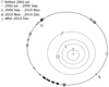 |
Fig. 1 Distribution of observations (see Table A.1) of P/2016 G1 along its orbit. The symbols indicate the apparitions from aphelion (Q) to aphelion. Perihelion is marked (q). Filled symbols show when the comet was detected, open symbols where it was not detected. No observations were acquired during the 2002 July–2006 September apparition. The positions of the planet symbols correspond to 2016 July. |
3 Analysis and results
3.1 Surface brightness profiles
The pre-discovery data on P/2016 G1 with the PS1 telescope on 2016 March 7 consist of four images, showing the object with a stellar morphology. Only two of the frames had the object clear of the chip gap boundary. The surface brightness profile was computed ineach of these frames for P/2016 G1 and for three nearby field stars in order to assess whether there was any dust surrounding the nucleus. We compute the radial flux profile using the median per-pixel flux in circular annuli around the object, and convert the flux to surface brightness using the zeropoint in the PS1 headers. Errors are obtained using bootstrap re-sampling within each annulus. Figure 3 presents the average normalised surface brightness profile of both P/2016 G1 and the field stars, and shows that P/2016 G1 is more extended. During each exposure, the object moved about 0.′′ 3, which is significantly less than the seeing, meaning that trailing does not cause the flux excess seen in P/2016 G1. We conclude that the object was already surrounded by dust on 2016 March 7.
3.2 Description and nomenclature
Figure 2 shows a series of images of the object over time. The central structure of the object is composed of three main concentrations of dust forming an inverted “C” on the images (hereafter referred to as the three clumps), and a much fainter concentration on the eastern side, leaving a central gap. This structure grows with time, preserving its appearance. The central structure is bathed in a diffuse, elongated coma that extends into a dust tail westward from the central structure. The orientation of the coma and the tail is rotating southward as the viewing geometry evolves.
Below the central structure, a small, narrow, well-defined arc extends toward the south-southeast. This arc is clearly seen from April 3 until May 12 and is still detected on May 31. Directly eastward of the central structure, but not pointing toward its centre, a faint linear feature is present. It can also be seen until May 12. The arc and the linear features are marked on Fig. 2C.
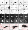 |
Fig. 2 Panels A: images of P/2016 G1 between UT 2016 March 7 and July 4. All the images are scaled to be 6 × 10⁴ km on a side. The Earth crossed the orbital plane of the object on April 13, so images around that date show the coma extension above and below the plane. Panels B: images of P/2016 G1 processed with unsharp masking to enhance the three clumps and the details near the disintegrating body. Each image is 1.5 × 10⁴ km on a side. Panels C: contour plots on three dates showing the expansion of the southern arc and the eastern linear feature (highlighted with red lines). Each panel is 30″ × 20″. The panel widths and pixel scales are: April 3 (34 000 km, 227 km), April 14 (32 000 km, 231 km), and May 12 (29 000 km, 193 km). North is up, east is left. The Sun and velocity vectors are listed in Table A.1. |
3.3 Main head dust feature
The Earth crossed the orbital plane of the comet on 2016 April 13. The images taken around that date indicate that the complex head structure and the central coma extend above and below the orbital plane, whose orientation corresponds on the images to that of the tail feature (PA = 274°). The grains forming the head structure must therefore have been ejected with a non-zero velocity, with a non-zero component perpendicular to the orbital plane.
The size of the central structure was estimated measuring the distance between the peak of the north and south concentrations. When the peak is not well defined, the centre of the concentration was used instead. These angular distances were converted to a linear distance in the plane of sky accounting for the geocentric distance (and reported in Fig. 4). In the March 7 image, although the object is broader than stellar, the central structure is not yet resolved. The diameter of the seeing disk is therefore used as an upper limit. The size of the structure grew linearly with time. A linear regression indicates that the growth would have started on 2016 March 6 (JD = 2457454) ± 3 days, and is expanding with an average (plane of sky) velocity of 0.32 ± 0.02 m s−1 (i.e., drifting from the centre of the original object at half that speed). The March 7 image would therefore have been obtained very soon after the onset of the activity, and the observed broadening of the image could be caused by the cloud of fine dust expanding more rapidly than the larger fragments.
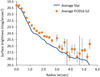 |
Fig. 3 Average surface brightness profile of P/2016 G1 compared to the average profile for field stars as seen in the data obtained with the Pan-STARRS1 telescope on 2016 March 7. The profiles for the field stars have been normalised to the peak brightness for P/2016 G1. Although the images of the comet appear stellar in the images, its profiles indicate that the object isslightly –but significantly– extended. |
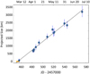 |
Fig. 4 Size of the main head structure as a function of time. The line and the horizontal error bar indicate the linear expansion fitted to the data and the error on the origin, 2016 March 6 ± 3 days. |
3.4 Finson–Probstein dust modelling
The positions of the Earth, the comet, and the Sun in late May and in June show the dust features of the tail with a geometry very favourable for a Finson–Probstein (FP, Finson & Probstein 1968; Farnham 1996) dust dynamical analysis. Finson–Probstein modelling calculates the trajectories of an ensemble of dust grains of different sizes, parameterised by β (ratio between theradiation pressure and the solar gravity) ejected from the surface of the nucleus at different times, τ, as acted upon by solar gravity and solar radiation pressure. We used the FP approach to analyse the pattern of synchrones (loci of the particles emitted at the same time) and syndynes (curves joining particles with the same β) and the optical appearance of the dust environment of the comet.
The main tail-like feature has a fairly sharp profile in azimuth as shown in Fig. 5. The position angle of the peak was measured on the images; it is marked as a thick line on the FP plots. The epoch of the corresponding synchrone was obtained by comparing the position angles of synchrones generated with a step of 1 day. The error on that epoch resulting from the measurement uncertainty is ±3 days. The azimuthal profile of the tail is very roughly Gaussian; converting the FWHM (measured using the same procedure as above), this also results in a “σ” of ±3 days. The broadening of the tail is caused in part by the seeing (negligible far from the nucleus), by the dispersion in emission velocity (which is neglected in the zero-velocity FP method), and by the duration of the dust emission. The broadening caused by the emissionvelocity can be estimated from the images obtained when the Earth was close to the orbital plane (when the synchrones and syndynes degenerate into a single line), around April 13 (see Fig. 2): the width of the tail on April 14 is similar to that seen on April 4–8, when the orbital plane was observed at an angle. We conclude that the broadening of the tail is dominated by the velocity dispersion of the grains (which occurs in all directions, including perpendicular to the orbital plane), rather than purely by the radiation pressure (which occurs only within the orbital plane).
The tail-like feature is therefore compatible with a burst of dust emission centred on 2016 March 4 ± 3 days for the image from 2016 May 31, and 2016 March 7 ± 3 days for the image from 2016 June 8. The emission profile is compatible with a short, impulsive burst smeared out by a distribution of initial velocities of the particles with v < 1 m s−1 in random directions, or a longer burst (increasing then decreasing over a few days) with no initial velocity. Furthermore, dust is present in the areas of the image not covered by the syndynes and synchrones, confirming that the dust must have been emitted with some initial velocity. We therefore favour the short, impulsive burst.
It is interesting that two independent measurements for the date of the onset of disintegration, namely the FP estimates and the central feature growth, are in perfect agreement.
Assuming that the tail-like structure is dominated by dust emitted with zero velocity, the spread of the dust along the tail is caused only by the radiation pressure. Close to the head of the object, the actual velocity dispersion of the grains will smear this relation, but further away, β (the ratio between the radiation pressure and the solar gravitation for the considered grain), a (the grain radius) and ρ (its density) are related by:
 (1)
(1)
where Qpr is a radiation pressure efficiency coefficient in the 1–2 range for rocky and icy material. With this relation, we can estimate the characteristic grain sizes in the images: with ρ = 3000 kg m−3 and Q = 1.05, Eq. (1) gives a = 2 × 10⁻⁷∕β (m). The loci of 10–200 μm grains are marked on Fig. 5. Closer to the head than the 100 μm mark, the blurring by the seeing and the non-zero velocity of the grains forming the head structure prevent FP from making meaningful estimates of the grain size beyond “they are large”, that is, in the millimetre range or even larger.
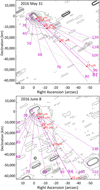 |
Fig. 5 Syndynes (in green) and synchrones (in purple, labelled in days before the observation date) for P/2016 G1 on 2016 May 31 and 2016 June 8. The thicker synchrone marks the brightest peak in the dust profile, and the corresponding grain radii are marked in red. This fits with the disruption taking place around March 6. |
3.5 Dynamical model of the arc and linear feature
In order to further investigate the structure of the head, we simulated the trajectory of large particles (i.e., not influenced by radiation pressure, β = 0), emitted from the position of the nucleus on 2016 March 6 with velocity values ranging from 0 to 3 m s−1, and directions covering the whole sphere every 2.5° in longitude and latitude (cometocentric coordinates, x and y in the orbital plane, y pointing toward the Earth). The position of each particle was computed for 2016 April 3, May 12, and May 31. The particles that were located at the position of the three fragment clumps, the southeast arc, and the start of the linear feature are identified, as illustrated in Fig. 6. Figure 7 shows the maps of the particles matching the features (in cometocentric longitude and latitude at the time of the emission), for a set of emission velocities.
The three main fragment clumps can be reproduced by particles emitted at any velocity between 0.25 and 3 m s−1. However, for higher velocities, they must be emitted almost exactly toward or away from Earth (so that the foreshortening keeps them at their position near the origin), which is unlikely. It is more likely that they were emitted at a random angle, that is, at velocities < 1 m s−1.
The southeast arc cannot have been emitted at velocities < 2.25 m s−1: part of the arc is not reproduced (some of the dots are missing). For velocities in the 2.25–3 m s−1 range, the complete feature can be reproduced by particles emitted at the same velocity. A cone with a half-opening of 40°, whose axis points toward cometocentric coordinates (long., lat.) = (68°, −15°) is found to accurately reproduce the arc feature and the start of the linear feature, with a velocity of 2.5 m s−1: the arc and the clump at the head of the linear features are on a ring corresponding to the 2.5 m s−1 slice of this same cone.
In order to test the validity of this interpretation, the position of the particles was also computed for April 3 and May 31, when the viewing geometry was very different. As illustrated in Fig. 8, the same ring of dust closely matches the 3D position and evolution of the arc and the head of the linear feature.
Adjusting the position and opening of the cone (by eye) gives an estimate of the uncertainty on these parameters: ± 2.5° in longitude and latitude, and ± 5° in opening. Changing the opening of the cone also slightly modifies the velocities of the particles matching the features. The date of the initial burst was also changed by 5, 10, and 15 days. No effect is noticeable for five-day change; a slight change of orientation and velocity is required for the changes of 10 and 15 days. This therefore does not set additional constraints on the time of the emission.
Using the FP formalism (Sect. 3.4), the trajectory of small dust grains emitted together with the larger grains was calculated accounting for the radiation pressure. The smaller grains form a line (synchrone) starting at the large particle, and drifting away at an angle set by the emission date (while the large particles move on a straight line in the image plane, from the nucleus toward their observed position, the small particles start tangentially to that line, and drift on a parabolic trajectory toward their observed position). The eastern linear feature closely matches the position of small grains emitted at the same time, in the same direction, and at the same velocity as the clump at the head of the linear feature. They are highlighted with red dots in the May 12 panel of Fig. 8. Similarly, various clumps in the arc feature have similar “tails”, which together cause an enhancement of surface brightness on the western side of the arc (two of them are highlighted with red dots in the May 12 panel of Fig. 8). As the position angle of these synchrone lines is set only by the time of the emission, the excellent match between the eastern linear feature and the synchrone for a March 6 emission gives very strong support to the hypothesis that it corresponds to small grains emitted simultaneously and in the same direction as the big grains, and further supports the March 6 emission date. It also rules out that the linear feature would have been caused by a secondary disruption of a large grain at a later date: the position angle of the corresponding synchrone would have been different.
Overall, the southern arc and the head of the eastern linear feature are large particles partially populating a ring. The arc covers at least a quarter of the ring, possibly more, as its northern part is lost in the main coma. A single clump of large particles on the ring forms the tip of the eastern linear feature. This ring grows in size with time, as the particles move away from the emission spot at (2.5 ± 0.1)m s−1, describing a cone with a half-opening of 40°.
It is possible that the sections of the ring that appear devoid of dust were originally populated by small grains: solar radiation pressure would have pushed them away from the field of view.
The ring corresponds to a very narrow velocity distribution: in particular, the “walls” of the cone are not populated by dust grains, only a (partial) ring.
We tried and failed to reproduce the arc and the eastern linear feature using dust grains emitted along a great circle in cometocentric coordinates, as would have been produced by an equatorial centrifugal ejection. We also tried and failed to reproduce the observed features using grains with a broader range of velocities: a velocity distribution around 2.5 m s−1, narrower than 0.125 m s−1, gives the best results.
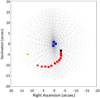 |
Fig. 6 Positions of large particles emitted by the nucleus on 2016 March 6, with velocities ranging from 0 to 3 m s−1 observed on 2017 May 12 marked with light grey dots in the plane of sky. The coordinates mark offsets from the position of the nucleus for that time. For clarity, only a subset of the particles is plotted. The particles matching the position of the three head features are marked in blue. Those matching the arc are marked in red (the ends of the feature are marked in magenta and black); the blob at the western start of the linear feature (Fig. 2) is marked in orange. |
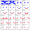 |
Fig. 7 For a series of emission velocity, maps of the emission direction (in cometocentric longitudes and latitudes) of the large particles matching the features observed on May 12, using the same colour code as in Fig. 6. For any velocity, a particle matching a feature always has a “mirror particle”: one is emitted toward the Earth, the other one away from the Earth. On the 2.375, 2.5, and 2.625 m s−1 panels, the position of a 40° half-opening cone matching best the feature is represented. The direction directly toward Earth is marked by a black cross, away from Earth by a red cross, at 0° latitude, and 90° and 270° longitude, respectively. Re-projecting these maps onto concentric spheres, with the geometry of May 12, would lead to Fig. 6. |
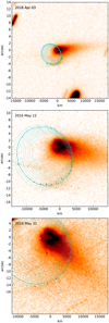 |
Fig. 8 P/2016 G1 on 2016 April 3, May 12, and May 31. The green dots mark clumps on the arc feature. The small red dots correspond to the synchrone trajectories of small dust (submitted to radiation pressure) emitted from some of the clumps on March 6. The position of large particles emitted on March 6 on a cone with half-opening 40° and centred on (long., lat.) = (68°, −15°) are over-plotted for velocities ranging from 1.625 to 2.750 m s−1. The solid line corresponds to 2.5 m s−1. |
3.6 The Moreno model
Moreno et al. (2016) obtained data for P/2016 G1 on three nights between 2016 April 20 and June 8 and used Monte Carlo techniques to model the dust. They obtained two additional epochs with the Hubble Space Telescope on 2016 June 28 and July 11 (Moreno et al. 2017).
Comparing the original dataset to model images generated using Monte–Carlo emitted particles following a FP-like formalism, these latter authors infer that the dust ejection began around 2016 February 10 , and decreased with a half-Gaussian function with a half-width at half maximum (HWHM) of
  d, corresponding to an emission of 1.7 × 10⁷ kg of dust, of which some was preferentially ejected in the westward direction, consistent with an impact aligned with the sun-asteroid vector. They inferred very low dust velocities with average speeds around 0.8 m s−1 and grain sizes between 1 μm and 1 cm in radius (the velocities in the original paper Moreno et al. 2016 had a typo, corrected in an erratum Moreno et al. 2019). The more recent HST data are compatible with their original model.
The analysis in Moreno et al. (2016) was focused on what we call here the central structure with the three main concentrations forming the inverted C on the images and the central dust coma. From an FP analysis similar to that of Sect. 3.4, these latter authors set the interval for the beginning of activity in their model from 2016 January 31 to April 1.
Our estimate of the date of the peak of dust emission relies on two simple and independent measurements: (i) the linear growth of the separation between the condensations in the central structure, which agrees with the barely resolved image obtained on March 7 (Sect. 3.1), and (ii) the position angle of the sharp cusp in the isophotes far from the origin, in Fig. 5. Measuring this angle in Fig. 2 of Moreno et al. (2016), we get very good agreement with our estimate. This makes the simple assumption that far from the origin, the effect of the radiation pressure dominates over an initial velocity. Moreno et al. ran their Monte-Carlo multi-parameter model to refine the combination of initial velocity and radiation pressure, leading to a difference in emission time of about a month. Their analysis does not mention the southern arc, nor the eastern linear features, whose geometry we find to strongly and independently confirm the emission date provided by the orientation of the main tail and the growth of the central structure, and to also support a very brief emission. This is further confirmed by the very narrow eastern linear feature, that points precisely at an impulsive emission on again the same date, March 6. Because of the convergence of these independent arguments, because they are based on much wider features than those Moreno et al. worked on, and because of the simplicity of the underlying assumptions, we are confident that the disruption occurred on 2016 March 6 ± 3 days.
In terms of duration, the analysis of Moreno et al. suggests that “[an] impact would have induced a partial destruction of the asteroid,” causing the anisotropic part of the dust emission, “with dust grains being emitted to space nearly isotropically while the body is being torn apart”, and that this isotropic emission would have had a duration of  d HWHM. Our data directly support the impact-induced destruction of the asteroid, the arc and linear feature being the signature of that impact. Concerning the broad dust feature on which Moreno et al. focus their study, our interpretation is that the broadening of the tail matches the dust velocity dispersion, and that therefore it is compatible with a very short duration event, although we cannot rule out (nor constrain) a longer duration for the final crumbling of the asteroid.
3.7 Massof the debris cloud
Because the exact grain size distribution present in each pixel of the image is not known, and because the central structure could contain verylarge particles (meter-sized or more), getting an evaluation of the mass of the object is difficult. This is made worse by the fact that larger particles contribute more to the mass, while smaller particles contribute more to the flux. Below we present an attempt to get a rough estimate of this mass, based on the May 31 image. We assume a dust density ρ = 3000 kg m−3, and an albedo p = 0.25.
To get an order-of-magnitude estimate, one can consider a uniform size distribution across the whole object (a power law with a − 3 index, and a cut-off at 1 cm, after Moreno et al. 2016). This leads to a total mass in the object of 1 × 10⁷ kg, in agreement with Moreno et al. who obtained an ejected mass of 2 × 10⁷ kg with their detailed model.
As we consider that the dust release event was short, the dust distribution (far from the position of the nucleus) is dominated by the radiation pressure: smaller grains are pushed further away than larger ones. While this estimate is also a simplification, it takes into accountthe fact that the dust is not uniformly distributed. The grain size is set using the scaling between size and distance from Fig. 5. The image is then integrated on concentric rings, and the flux is converted to dust surface, and then to the number of grains, and then into mass, as illustrated in Fig. 9. This results in a total mass for the object MN = 1.1 × 10⁹ kg. This estimate is still a lower limit, as larger clumps could hide in the central concentration. The mass corresponds to a spherical object with a radius RN ~ 44 m, well below the limit of detection of the pre-discovery images (RN < 200 m).
We do not know whether the object was completely disrupted. Using their high-resolution, deep HST images, Moreno et al. (2017) obtained an upper limit of 30 m to the fragments. The mass potentially contained in even a few of these large fragments would completely dominate the mass of the dust. In what follows we consider as a lower limit the mass of the dust (and the corresponding radius RN > 44 m), and the upper limit from the pre-discovery constraints (RN < 200 m), with most of the mass being located in the central concentration, which we observed expanding at v = 0.16 m s−1. The corresponding kinetic energy is K = 1.4 × 10⁷ and 1.3 × 10⁹ J for RN = 44 and RN = 200 m, respectively. In order to reach this asymptotic velocity, the grains and fragments had to overcome the (small) gravity potential of the object, with an escape velocity 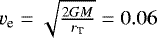 and 0.26 m s−1, respectively.This implies that the disruption of the object required a total energy at least
 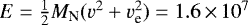 and 4.7 × 10⁹ J, respectively.These are clearly lower limits that consider a pure rubble pile, that is, without any internal cohesion forces.
Considering that this energy was provided by an impactor, and that collision happened at the median impact velocity in the main belt vi = 5000 m s−1, this requires a tiny impactor of 1 kg, with a radius of 5 cm for the lower limit on the object size, and 370 kg with a radius of 30 cm for the larger object.
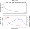 |
Fig. 9 Top: radius of the dust grains as a function of the distance to the centre of the object, using the FP scaling (see Sect. 3.4 and Fig. 5) for May 31. Bottom: flux in the May 31 image is integrated over concentric rings and converted into the number of particles (blue) and the mass (red), both in each radial bin. |
3.8 Summary of the analysis
Overall, our results are based on various independent measurements and a separate simple interpretation points toward the following scenario:
-
No image from before 2016 March shows the object. These non-detections lead to a radius RN < 0.2 km.
-
The onset of activity was on 2016 March 6. Backward extrapolation of the central structure gives an uncertainty of ±3 days but the object was found active on March 7. This March 6 date is confirmed by the following independent measurements: the orientation of the azimuthal peak of the main tail; the position and evolution of the southern arc and of the head of the linear feature; and the orientation of the eastern linear feature.
-
The dust emission event had a very brief component (indicated by the narrow eastern linear feature and the narrow ring of large particles populating the southern arc), which may possibly have been followed by a longer emission of dust from the central feature.
-
The central component of the object is composed of large dust grains moving at low velocity (0.16 ± 0.01 m s−1 in the plane of sky) from the original centre. It is surrounded by a cloud of smaller particles, also emitted at similar low speed, and being pushed away by radiation pressure. The visible tail is populated by particles in the 10–200 μm range. Larger particles are certainly present, but cannot be distinguished in the central component, with smaller particles drifting away from the field of view. The broadening of the March 7 image could be caused by the hyper-velocity material released during the impact itself, while the slower material was released during the follow-up disruption.
-
During the brief emission event, a group of particles was emitted on a cone with a half-opening angle of 40 ± 5°, propagating at (2.5 ± 0.1) m s−1 and forming part of a ring, with an arc covering over a quarter of the ring plus a clump opposite to the arc (forming the southernarc and the head of the eastern linear feature). The large particles were emitted together (in time, direction, and velocity) with smaller particles, which are seen drifting from the ring under the radiation pressure. They form the eastern linear feature and a faint westward extension to the southern arc. These features could not have been reproduced by emission on a grand circle (matching, for instance, an equatorial ejection).
4 Discussion: impact and disruption
From the observations, a major disruption occurred on P/2016 G1 on or around 2016 March 6, disrupting –possibly destroying – the object, and releasing a ring of large particles moving at ~ 2.5m s−1, growing on acone with a half-opening angle of ~40°. We consider the impact of a metre-scale object hitting a 100-metre-scale asteroid at ~ 5 km s−1. All the hyper-velocity ejecta which would be expanding at impact-scale speeds (in the km s−1 range) have moved degrees away from the position of the object at the time of the first deep images (about one month after the impact). Radiation pressure having further dispersed these grains, they are lost beyond the field of view of the observations.
All that is left in the field of view are the spalls and large dis-aggregated fragments of the objects that came off well after the impact, in the final stages of the formation of the crater and after, together with the dust grains released. Crater formation simulations (numerical and laboratory) show that asymmetries in the filling of the ejection cone are common; this would explain why the ring is not complete.
These grains (>10 μm) are either the small end of a power-law size-distribution of the fragments, and/or the regolith that was dragged along with bigger fragments. The bulk of the energy of the impactor is transferred into the bulk of the body, causing its disruption into fragments that drift apart at very low velocities.
Hydrodynamic simulations of impacts can provide information on the remnants, in particular on their size distribution (see Durda et al. 2007, for a systematic study of various parameters) and velocities. Simulations of catastrophic impacts3 show that the plate-shaped spall fragments, corresponding to the final moments of the crater formation, are ejected with different velocities and over a broad range of directions. However, the crater formation process also produces wedge-shaped fragments, bounded by the propagating radial cracks. These have a narrow distribution of slow velocity, in the metres-per-second range, and are axially isotropic about the point of impact. These large wedges would become visible as they break apart and their surface area increases. Based on these qualitative arguments, we suggest that the feature we interpret as a ring of fragments corresponds to what remains of these large wedge-shaped fragments. Hydrodynamics simulations, beyond the scope of this paper, will be used to quantitatively verify the plausibility of this hypothesis. Interestingly, the velocity of ejection of these wedge-shaped fragments is directly linked to the tensile strength of the object. The tensile strength is one of the key structural characteristics of an asteroid, but it is normally not accessible remotely. In the case of a rotationally disrupted asteroid, the study of the fragmentation can cast some light on the internal strength, but with some uncertainties caused by the unknown initial spin of the object (see Hirabayashi et al. 2014, for an application to rotationally disrupted P/2013 R3). A result of the ongoing simulation will therefore be the first direct remote estimate of the tensile strength of an asteroid, a measurement that would have implications for the mitigation measures being investigated for planetary defence initiatives.
Acknowledgements
We are very grateful for the detailed review and comments provided by the referee, Fernando Moreno. K.J.M., J.K., and J.V.K. acknowledge support through an award from the National Science Foundation AST1413736. R.J.W. acknowledges support by NASA under grant NNX14AM74G. This paper is based on observations obtained with MegaPrime/MegaCam, a joint project of CFHT and CEA/DAPNIA, at the Canada-France-Hawaii Telescope (CFHT) which is operated by the National Research Council (NRC) of Canada, the Institut National des Sciences de l’Univers of the Centre National de la Recherche Scientifique of France, and the University of Hawaii. Data were acquired using the PS1 System operated by the PS1 Science Consortium (PS1SC) and its member institutions. We thank the staff of IAO, Hanle and CREST, Hosakote, that made these observations possible. IAO and CREST are operated by the Indian Institute for Astrophysics, Bangalore. The Pan-STARRS1 Surveys (PS1) have been made possible by contributions from PS1SC member Institutions and NASA through Grant NNX08AR22G, the NSF under Grant No. AST-123886, the Univ. of MD, and Eotvos Lorand Univ. We would like to thank Detlef Koschny (ESA) and Mikael Granvik for their helpful discussion on impact cratering mechanics and disruption. This research was supported by the Munich Institute for Astro- and Particle Physics (MIAPP) of the DFG cluster of excellence “Origin and Structure of the Universe”.
Appendix A Table
Observations.
References
- Benavidez, P. G., Durda, D. D., Enke, B. L., et al. 2012, Icarus, 219, 57 [NASA ADS] [CrossRef] [Google Scholar]
- Bertin, E., & Arnouts, S. 1996, A&AS, 117, 393 [NASA ADS] [CrossRef] [EDP Sciences] [Google Scholar]
- Carruba, V., Nesvorný, D., Marchi, S., & Aljbaae, S. 2016, MNRAS, 458, 1117 [CrossRef] [Google Scholar]
- Durda, D. D., Bottke, W. F., Nesvorný, D., et al. 2007, Icarus, 186, 498 [NASA ADS] [CrossRef] [Google Scholar]
- Farnham, T. L. 1996, PhD Thesis, University of Hawai’i, Honolulu, Hawaii, USA [Google Scholar]
- Finson, M. J., & Probstein, R. F. 1968, ApJ, 154, 327 [NASA ADS] [CrossRef] [Google Scholar]
- Gwyn, S. D. J., Hill, N., & Kavelaars, J. J. 2012, PASP, 124, 579 [NASA ADS] [CrossRef] [Google Scholar]
- Hirabayashi, M., Scheeres, D. J., Sánchez, D. P., & Gabriel, T. 2014, ApJ, 789, L12 [NASA ADS] [CrossRef] [Google Scholar]
- Hsieh, H. H., Novaković, B., Kim, Y., & Brasser, R. 2018, AJ, 155, 96 [CrossRef] [Google Scholar]
- Milani, A., Knežević, Z., Spoto, F., et al. 2017, Icarus, 288, 240 [NASA ADS] [CrossRef] [Google Scholar]
- Moreno, F., Licandro, J., Cabrera-Lavers, A., & Pozuelos, F. J. 2016, ApJ, 826, L22 [NASA ADS] [CrossRef] [Google Scholar]
- Moreno, F., Licandro, J., Mutchler, M., et al. 2017, AJ, 154, 248 [CrossRef] [Google Scholar]
- Moreno, F., Licandro, J., Cabrera-Lavers, A., & Pozuelos, F. J. 2019, ApJ, 877, L41 [CrossRef] [Google Scholar]
- Tonry, J. L., Stubbs, C. W., Lykke, K. R., et al. 2012, ApJ, 750, 99 [NASA ADS] [CrossRef] [Google Scholar]
- Weryk, R., Wainscoat, R. J., Micheli, M., & William, G. V. 2016, CBAT, 4269, 1 [Google Scholar]
All Tables
All Figures
|
Fig. 1 Distribution of observations (see Table A.1) of P/2016 G1 along its orbit. The symbols indicate the apparitions from aphelion (Q) to aphelion. Perihelion is marked (q). Filled symbols show when the comet was detected, open symbols where it was not detected. No observations were acquired during the 2002 July–2006 September apparition. The positions of the planet symbols correspond to 2016 July. |
| In the text | |
|
Fig. 2 Panels A: images of P/2016 G1 between UT 2016 March 7 and July 4. All the images are scaled to be 6 × 10⁴ km on a side. The Earth crossed the orbital plane of the object on April 13, so images around that date show the coma extension above and below the plane. Panels B: images of P/2016 G1 processed with unsharp masking to enhance the three clumps and the details near the disintegrating body. Each image is 1.5 × 10⁴ km on a side. Panels C: contour plots on three dates showing the expansion of the southern arc and the eastern linear feature (highlighted with red lines). Each panel is 30″ × 20″. The panel widths and pixel scales are: April 3 (34 000 km, 227 km), April 14 (32 000 km, 231 km), and May 12 (29 000 km, 193 km). North is up, east is left. The Sun and velocity vectors are listed in Table A.1. |
| In the text | |
|
Fig. 3 Average surface brightness profile of P/2016 G1 compared to the average profile for field stars as seen in the data obtained with the Pan-STARRS1 telescope on 2016 March 7. The profiles for the field stars have been normalised to the peak brightness for P/2016 G1. Although the images of the comet appear stellar in the images, its profiles indicate that the object isslightly –but significantly– extended. |
| In the text | |
|
Fig. 4 Size of the main head structure as a function of time. The line and the horizontal error bar indicate the linear expansion fitted to the data and the error on the origin, 2016 March 6 ± 3 days. |
| In the text | |
|
Fig. 5 Syndynes (in green) and synchrones (in purple, labelled in days before the observation date) for P/2016 G1 on 2016 May 31 and 2016 June 8. The thicker synchrone marks the brightest peak in the dust profile, and the corresponding grain radii are marked in red. This fits with the disruption taking place around March 6. |
| In the text | |
|
Fig. 6 Positions of large particles emitted by the nucleus on 2016 March 6, with velocities ranging from 0 to 3 m s−1 observed on 2017 May 12 marked with light grey dots in the plane of sky. The coordinates mark offsets from the position of the nucleus for that time. For clarity, only a subset of the particles is plotted. The particles matching the position of the three head features are marked in blue. Those matching the arc are marked in red (the ends of the feature are marked in magenta and black); the blob at the western start of the linear feature (Fig. 2) is marked in orange. |
| In the text | |
|
Fig. 7 For a series of emission velocity, maps of the emission direction (in cometocentric longitudes and latitudes) of the large particles matching the features observed on May 12, using the same colour code as in Fig. 6. For any velocity, a particle matching a feature always has a “mirror particle”: one is emitted toward the Earth, the other one away from the Earth. On the 2.375, 2.5, and 2.625 m s−1 panels, the position of a 40° half-opening cone matching best the feature is represented. The direction directly toward Earth is marked by a black cross, away from Earth by a red cross, at 0° latitude, and 90° and 270° longitude, respectively. Re-projecting these maps onto concentric spheres, with the geometry of May 12, would lead to Fig. 6. |
| In the text | |
|
Fig. 8 P/2016 G1 on 2016 April 3, May 12, and May 31. The green dots mark clumps on the arc feature. The small red dots correspond to the synchrone trajectories of small dust (submitted to radiation pressure) emitted from some of the clumps on March 6. The position of large particles emitted on March 6 on a cone with half-opening 40° and centred on (long., lat.) = (68°, −15°) are over-plotted for velocities ranging from 1.625 to 2.750 m s−1. The solid line corresponds to 2.5 m s−1. |
| In the text | |
|
Fig. 9 Top: radius of the dust grains as a function of the distance to the centre of the object, using the FP scaling (see Sect. 3.4 and Fig. 5) for May 31. Bottom: flux in the May 31 image is integrated over concentric rings and converted into the number of particles (blue) and the mass (red), both in each radial bin. |
| In the text | |
Current usage metrics show cumulative count of Article Views (full-text article views including HTML views, PDF and ePub downloads, according to the available data) and Abstracts Views on Vision4Press platform.
Data correspond to usage on the plateform after 2015. The current usage metrics is available 48-96 hours after online publication and is updated daily on week days.
Initial download of the metrics may take a while.