| Issue |
A&A
Volume 690, October 2024
|
|
|---|---|---|
| Article Number | A298 | |
| Number of page(s) | 13 | |
| Section | Planets and planetary systems | |
| DOI | https://doi.org/10.1051/0004-6361/202451090 | |
| Published online | 18 October 2024 | |
Activity of main-belt comet 324P/La Sagra
1
Institut für Geophysik und Extraterrestrische Physik, Technische Universität Braunschweig,
Mendelssohnstraße 3,
38106
Braunschweig,
Germany
2
Max Planck Institute for Solar System Research,
Justus-von-Liebig-Weg 3,
37077
Göttingen,
Germany
3
Department of Earth, Planetary and Space Sciences, UCLA,
Los Angeles,
CA
90095-1567,
USA
4
Planetary Science Institute,
1700 East Fort Lowell Road, Suite 106,
Tucson,
85719,
USA
★ Corresponding author; This email address is being protected from spambots. You need JavaScript enabled to view it.
Received:
12
June
2024
Accepted:
5
September
2024
Abstract
Aims. We study the activity evolution of the main-belt comet 324P/La Sagra over time and the properties of its emitted dust.
Methods. We performed aperture photometry on images taken by a wide range of telescopes at optical and thermal infrared wavelengths between 2010 and 2021. We derived the combined scattering cross section of the nucleus and dust (when present) as a function of time, and we derived the thermal emission properties.
Results. Fitting an IAU H-G phase function to the data obtained when 324P was likely inactive, we derived an absolute nucleus magnitude HR = (18.4 ± 0.5) mag using G = 0.15 ± 0.12. The activity of 324P/La Sagra during the 2015 perihelion passage has significantly decreased compared to the previous perihelion passage in 2010, and it decreased even further during the 2021 perihelion passage. This decrease in activity may be attributed to mantling or to the depletion of volatile substances. The A f ρ profile analysis of the coma of the main-belt comet suggests a near-perihelion transition from a lower-activity pre-perihelion to a higher-activity post-perihelion steady state. We calculate a dust geometric albedo in the range of (2–15)%, which prevents us from constraining the spectral type of 324P/La Sagra, but we found an indication of dust superheating at 4.5 μm.
Key words: methods: data analysis / techniques: photometric / comets: general / minor planets, asteroids: general / comets: individual: 324P/La Sagra
© The Authors 2024
 Open Access article, published by EDP Sciences, under the terms of the Creative Commons Attribution License (https://creativecommons.org/licenses/by/4.0), which permits unrestricted use, distribution, and reproduction in any medium, provided the original work is properly cited.
This article is published in open access under the Subscribe to Open model. This email address is being protected from spambots. You need JavaScript enabled to view it. to support open access publication.
1 Introduction
Active asteroids exhibit comet-like dust emission, but have asteroid-like orbits (with a Tisserand parameter with respect to Jupiter TJ ≳ 3, and with a location inside the Jupiter orbit). Main-belt comets (MBCs) are a subgroup of active asteroids (Jewitt et al. 2015; Hsieh & Sheppard 2015). The dust emission in MBCs is due to ice sublimation (Hsieh et al. 2012a; Jewitt et al. 2015), while in active asteroids that are not driven by sublimation, it is due to events such as impacts (Jewitt et al. 2011; Bodewits et al. 2011; Ishiguro et al. 2011; Kim et al. 2017a,b) or rotational destabilization (Jewitt et al. 2013, 2014a; Drahus et al. 2015; Sheppard & Trujillo 2015). Observationally, MBCs are usually identified through the specific time-dependence of the activity: They are active near perihelion, and the activity continues for an extended period of time of at least a few weeks, and it recurs during successive perihelia. In non-MBC active asteroids, the activity can occur at any true anomaly and can consist of single-time events, but is not limited to them.
Currently, only the James Webb Space Telescope (JWST) has a sufficiently high sensitivity to spectroscopically detect water vapor near an MBC. The first such detection was reported for 238P/Read (Kelley et al. 2023). This was the first detection of water-outgassing from a main-belt object that also emits visible dust. Küppers et al. (2014) detected water-vapor plumes without associated dust from the dwarf planet Ceres.
In the absence of spectroscopic evidence, repeated and prolonged dust-emission activity in MBCs near perihelion is still considered a strong indicator of sublimation, because this behavior is difficult to explain as the direct result of other mechanisms (Hsieh et al. 2008, 2011, 2012a,b; Hsieh 2015; Moreno et al. 2011, 2013; Jewitt et al. 2014b; Pozuelos et al. 2015). However, the survival of primordial water ice in main-belt objects after billion-year timescales has been shown to be possible by numerical thermal models only when the ice is buried under a protective dusty layer (Fanale & Salvail 1989; Schorghofer 2008, 2016; Prialnik & Rosenberg 2009; Schörghofer & Hsieh 2018). Hence, MBC activity needs a trigger event to expose this buried ice to solar irradiation. One possible trigger may be collisions (Haghighipour et al. 2016, 2018). The dust emission of the MBCs is then driven by the sublimation of these recently exposed materials (Hsieh et al. 2004; Hsieh & Jewitt 2006). Direct ice exposure is not necessary to activate MBCs, because a mere reduction of the dust layer thickness at the bottom of a crater may be sufficient for the underlying ice to sublimate (Capria et al. 2012). Most MBCs have their peak activity after perihelion. This delay in the sublimation process may be due to the time needed for the thermal wave to reach the ice buried in the subsurface (Hsieh 2015).
However, fast rotation may also play a role in triggering ice sublimation and/or sustaining dust emission against gravity. For example, the activity of 133P/Elst-Pizarro, the first MBC discovered in 1996, may be due to the combined effects of an initial triggering impact, sublimation, and rapid rotation (Hsieh et al. 2004, 2010; Hsieh 2015; Jewitt et al. 2014b).
Numerical models show that the orbits of most MBCs are dynamically stable, indicating that these objects formed in the main asteroid belt (Haghighipour 2009; Jewitt et al. 2009; Hsieh et al. 2012a,b). There they would have been dormant for a long time until their recent activation (Hsieh et al. 2004; Capria et al. 2012). Some studies also suggested that MBC activation may be facilitated by the preceding collisional breakup of larger parent bodies that would leave subsurface ice at comparatively shallow depths (Hsieh et al. 2018b). However, the orbits of a few MBCs are unstable on timescales of 20–30 Myr, suggesting that they may have reached their current orbital locations through interactions with giant planets (Haghighipour 2009; Jewitt et al. 2009). Some MBCs may even have formed in the outer Solar System and been captured into the main asteroid belt (Haghighipour 2009; Hsieh & Haghighipour 2016; Kim et al. 2022).
The MBC 324P/La Sagra (hereafter 324P) was discovered in 2010 as P/2010 R2 (Nomen et al. 2010). Its prolonged dust emission and mass loss during different perihelion passages suggest that its activity is driven by sublimation (Moreno et al. 2011; Hsieh et al. 2012b; Bauer et al. 2012; Hsieh & Sheppard 2015). It is dynamically associated with the Alauda family (Hsieh et al. 2018b), meaning that the composition of 324P may be similar to that of the other Alauda family asteroids. The orbital elements of 324P are listed in Table 1.
In this work, we perform a photometric analysis of 324P during its 2010, 2015 and 2021 perihelion passages, and we compare our results to previous studies. In Sec. 2, we describe the image datasets used for this work. In Sec. 3, we report the methods and analyses applied to the image sets and present and discuss our results. We summarize the results in Sec. 4.
Parameters describing the orbit of 324P.
2 Observations
We studied archival data of 324P obtained between 2010 and 2020, and we observed it during its perihelion passage in 2021 (Fig. 1). 324P was at perihelion on 2010 June 25, 2015 November 30, and 2021 May 6 (UT).
Images captured at both optical and infrared (IR) wavelengths were identified using the Canadian Astronomy Data Centre (CADC) website1 (Gwyn et al. 2012) and from the Infrared Science Archive (IRSA) website2. All visible-light images used in our study were obtained in the R band, except for the Pan-STARRS (PS1) image dated 2010 June 26 (which is in the z band), four PS1 images from 2010 September 8 (g band), and Hubble Space Telescope (HST) images in F350LP filter, whose pivot wavelength (Marinelli & Dressel 2024) is at 587.39 nm, similar to the V band.
Images obtained with the Very Large Telescope (VLT) on 2019 April 12 have a signal-to-noise ratio of S/N < 8, and we therefore excluded them from the further analysis. We did not detect 324P in Zwicky Transient Facility (ZTF) images from 2019 April 9, 2019 April 12, 2019April 19, and 2019 April 28.
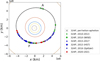 |
Fig. 1 Orbit plot in the heliocentric ecliptic coordinate system. The origin is the center of the Sun, the plane of reference is the ecliptic plane, and the direction of the x-axis points toward the vernal equinox. The plot shows the positions of 324P at the epochs of our observations with the orbits of Mercury, Venus, Earth, Mars, 324P, and Jupiter. Crosses represent the perihelion (P) and aphelion (A) positions. Pentagons, triangles, squares and circles represent visual data, and diamonds and stars are IR data. (The plot was generated using the poliastro Python library; Juan Luis Cano Rodríguez & Jorge Martínez Garrido 2022.) |
2.1 Visible-light data
Visible-light images of 324P (Fig. A.1) were obtained with the telescopes and instruments listed in Table A.1. We performed bias subtraction and flat-fielding using the following software packages: Dragons for Gemini data, Image Reduction and Analysis Facility (IRAF; Tody 1986, 1993) to process New Technology Telescope (NTT) data, and EsoRex for VLT data. The Pan-STARRS data were processed by the PS1 Image Processing Pipeline (Magnier 2006). Isaac Newton Telescope (INT) data were processed by the INT Wide Field Camera pipeline (Irwin & Lewis 2001). Canada-France-Hawaii Telescope (CFHT) data were processed by the Elixir pipeline (Magnier & Cuillandre 2004). Lowell Discovery Telescope (LDT) data were received in private communication from Matthew M. Knight in a post-processed state. For the HST data, we computed the target magnitude using the relation
![Mathematical equation: $\[V=20{-}2.5 ~\log _{10}\left[\frac{f}{n}\right],\]$](/articles/aa/full_html/2024/10/aa51090-24/aa51090-24-eq1.png) (1)
(1)
which we obtained from the Exposure Time Calculator (ETC) for the Wide Field Camera 3 (WFC3) Ultraviolet-Visible (UVIS) channel3. V is the apparent magnitude in the V band, f is the count rate of the source in e− s−1, and n is the count rate4 obtained by the ETC with the F350LP filter from a source with a Sun-like (Kurucz G2V) spectrum renormalized to Vega magnitude 20 in the Johnson/V filter.
For the CFHT and PS1 images, we used zero points computed by the Elixir and PS1 IPP pipelines, respectively. For data from all other instruments, we performed a photometric calibration relative to field stars from the PS1 catalog5. We also applied this method to the CFHT and PS1 data to check for consistency within our dataset, which we confirmed. We assumed solar colors for the conversions between the different PS1 bands r − z = 0.5 and r − g = −0.62 (Tonry et al. 2012; Willmer 2018), and for the conversion from the V to R band, V − R = 0.35 (Holmberg et al. 2006; Jewitt et al. 2016).
With IRAF, we performed photometry on single images of 324P using a circular aperture with a fixed physical radius of 2300 km at the comet. We opted for a constant physical radius (as opposed to constant angular size) to capture the same volume around the nucleus in every measurement. Subsequently, we calculated the weighted average of the apparent magnitudes measured on single exposures for each dataset, resulting in one measurement point per epoch and telescope (Table A.1). We performed circular aperture photometry on stacked HST images (Jewitt et al. 2016) with a fixed physical radius of 3000 km at the comet to ensure consistency in our comparative analysis with the Spitzer data (Section 2.2).
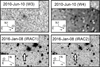 |
Fig. 2 IR images of 324P (at the center of each panel). The label W3 refers to WISE band 3 (12 μm), W4 to WISE band 4 (22 μm), and IRAC1 and IRAC2 corresponds to Spitzer Space Telescope observations at 3.6 μm and 4.5 μm, respectively. The dates and directions on sky are labeled as in Fig. A.1. |
2.2 Infrared data
Infrared images of 324P (Fig. 2) were taken on 2010 June 9–11 (true anomaly of ν = −3.9°, in the active phase) with the Wide-field Infrared Survey Explorer (WISE) telescope with a 0.4-meter diameter primary mirror (2.75″ per pixel in the W1 band at 3.4 μm, the W2 band at 4.6 μm, and the W3 band at 12 μm, 5.5″ per pixel in the W4 band at 22 μm). The WISE data were processed and photometrically calibrated by the WSDS PIPELINES (Cutri et al. 2012). To increase the S/N, we co-added images with the WISE Coadder software6.
We converted WISE magnitudes into fluxes using (Cutri et al. 2012)
![Mathematical equation: $\[F_\nu=F_{\nu 0} \cdot 10^{\left(-m_{V_{ega }} / 2.5\right)},\]$](/articles/aa/full_html/2024/10/aa51090-24/aa51090-24-eq2.png) (2)
(2)
where Fv is the flux density in Jy, Fv0 is the zero-magnitude flux density (Wright et al. 2010; Mainzer et al. 2011; Masiero et al. 2011), and mVega is the measured WISE Vega magnitude, all at frequency ν. We measured the dust brightness inside apertures with angular radii 11″ (corresponding to 19 230 km) for the W1, W2 and W3 bands, and 22″ (38460 km) for the W4 band (Bauer et al. 2012). We chose aperture values that were sufficiently larger than the point spread function (PSF) full width at half maximum (FWHM) of each band. For bands W1 and W2, we were only able to derive upper limits. Our results for all four bands are consistent with those of Bauer et al. (2012).
Infrared images were also taken on 2016 January 8 (ν = 9.8°, also in the active phase) with the Infrared Array Camera (IRAC) on the Spitzer Space Telescope with a 0.85-meter diameter primary mirror (1.22″ pixel−1 in channels 1 (3.6 μm) and 2 (4.5 μm)). Spitzer data were processed and calibrated by the IRAC pipeline (Fazio et al. 2004; IRAC Instrument and Instrument Support Teams 2021).
To assess the detectability of coma dust in Spitzer data, we measured the FWHM of the PSF of 324P and of isolated stars. We found 1.5 pixels < FWHM < 2 pixels for both 324P and the stars, indicating that the dust of the coma (if present) is unresolved. The Spitzer images (Fig. 2) are characterized by a crowded field of stars. For this reason we refrained from stacking the images and instead performed circular aperture photometry on single images with a fixed physical radius of 3000 km at the comet. To minimize the resulting flux uncertainty, we used small aperture sizes and selected images in which 324P did not overlap neighbouring stars.
To constrain the dust geometric albedo, we also estimated the brightness of 324P at the visible wavelengths (Fig. 3) at the epochs of our two IR observations (Table A.1). As the reference that is closest in time to the 2010 June 9–11 WISE observation, we identified a z-band PS1 image obtained on 2010 June 26. The absolute magnitude derived from this PS1 measurement inside an aperture with radius 3″ (4847 km) corresponds to an apparent z-band magnitude of (20.4 ± 1.4) mag, or to a flux of ![Mathematical equation: $\[0.02_{-0.01}^{+0.04}\]$](/articles/aa/full_html/2024/10/aa51090-24/aa51090-24-eq3.png) mJy, at the time of the WISE observation.
mJy, at the time of the WISE observation.
The visible-light reference data for the Spitzer epoch that are closest in time are four HST images in F350LP filter. To account for the increasing coma brightness between the individual HST observations, we extrapolated the absolute magnitudes to 2016 January 8, the epoch of the Spitzer measurement (Fig. 4) using a linear fit to the absolute magnitudes in Table A.1, We calculated the corresponding apparent magnitude at the position of Spitzer, finding a value of (20.9 ± 1.2) mag, and converted it into a flux of ![Mathematical equation: $\[0.02_{-0.01}^{+0.03}\]$](/articles/aa/full_html/2024/10/aa51090-24/aa51090-24-eq4.png) mJy using
mJy using
![Mathematical equation: $\[F=3.622 \cdot 10^{-5} \cdot 10^{\frac{20-V}{2.5}},\]$](/articles/aa/full_html/2024/10/aa51090-24/aa51090-24-eq5.png) (3)
(3)
where F is the flux of the source in Jy, 3.622 · 10−5 is the flux7 associated with a Vega magnitude of 20 in Johnson/V filter, and V is the measured magnitude in F350LP filter.
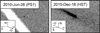 |
Fig. 3 Visual-light images (PS1 in the z band and HST in the V band) of 324P (at the center of each panel). The dates and directions on sky are labeled as in Fig. A.1. These visual images were obtained closest in time to the respective IR images shown in Fig. 2. |
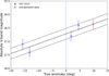 |
Fig. 4 Absolute V-band magnitudes of 324P plotted as a function of the true anomaly and linear fit for extrapolation. The blue dots show HST measurements, and the red dot shows the extrapolated value for 2016 January 8. The central solid line represents the fit to the data, and the dashed lines parallel to the solid line represent the uncertainty of the linear fit. |
3 Analysis and results
3.1 Nucleus magnitude
To assess the absolute magnitude of the bare nucleus of 324P, we exclusively analyzed data collected in 2013, when no activity was detected. We first normalized the measured average apparent R-band magnitudes, mR, to unit heliocentric (rh) and geocentric (Δ) distances using
![Mathematical equation: $\[m_{reduced}=m_R-5 ~\log _{10}\left(r_h \Delta\right) \text {, }\]$](/articles/aa/full_html/2024/10/aa51090-24/aa51090-24-eq6.png) (4)
(4)
where mreduced is the reduced R-band magnitude, and rh and Δ are measured in AU. The reduced magnitude is influenced by both the solar phase angle and the rotational phase of the nucleus at the time of observation. The rotation rate of the 324P nucleus is unknown, and our observations are too much scattered in time to constrain it. We fit the 2013 reduced magnitudes with an International Astronomical Union (IAU) H-G phase function, and because we lacked appropriate phase angle coverage, we assumed a default C-type value of G = 0.15 ± 0.12 (Bowell et al. 1989), which yielded HR = (18.4 ± 0.5) mag and is consistent with the HR = (18.4 ± 0.2) mag found by Hsieh (2014). Our assumed uncertainty of G is the standard deviation of many G values found by Lagerkvist & Magnusson (1990) (cf. Polishook & Brosch 2009). We plot our best-fit phase function in Fig. 5.
We calculated the effective nucleus radius using (e.g. Hsieh et al. 2023)
![Mathematical equation: $\[r_N{}^2=\frac{\left(2.24 \cdot 10^{16}\right) \cdot 10^{0.4\left(m_{\odot, R}-H_{R, {inactive}}\right)}}{p_R},\]$](/articles/aa/full_html/2024/10/aa51090-24/aa51090-24-eq7.png) (5)
(5)
where pR = 0.05 ± 0.02 is the assumed geometric R-band albedo (Hsieh et al. 2009; Hsieh et al. 2023), m⊙,R = −27.15 is the apparent R-band magnitude of the Sun, and HR,inactive is the absolute R-band magnitude of the inactive nucleus of (18.4 ± 0.5) mag. We found rN = (0.52 ± 0.16) km. This value agrees with the effective nucleus radius of ![Mathematical equation: $\[r_N=0.59_{-0.10}^{+0.18}\]$](/articles/aa/full_html/2024/10/aa51090-24/aa51090-24-eq8.png) km found in Hsieh et al. (2023), who assumed the same V-band albedo of pv = 0.05 ± 0.02.
km found in Hsieh et al. (2023), who assumed the same V-band albedo of pv = 0.05 ± 0.02.
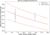 |
Fig. 5 Best-fit IAU phase function (solid red line) for 324P. The dashed red lines represent the uncertainty of the fit. The blue points show 2013 data, when the nucleus was inactive. These were used for the fit. |
3.2 Visible-light photometry of 324P in active state
The average absolute R-band magnitudes, HR, were calculated using (e.g. Hsieh et al. 2010)
![Mathematical equation: $\[H_R=m_{reduced}+2.5 ~\log _{10}\left[(1-G) \Phi_1(\alpha)+G \Phi_2(\alpha)\right],\]$](/articles/aa/full_html/2024/10/aa51090-24/aa51090-24-eq9.png) (6)
(6)
where α is the solar phase angle and the term (1 − G)Φ1(α) + GΦ2(α) is called the scattering phase function (Bowell et al. 1989). We also used G = 0.15 ± 0.12 (Sec. 3.1) for the dust. While there are measurements of the dust phase function for comets (Divine 1981; Schleicher 2010), we are not aware of a measured phase function for asteroid dust. Since there are indications that the dust properties for comets and asteroids are different (e.g. from comparing 67P measurements and Ryugu samples), we considered the nucleus phase function to be the most natural proxy for the unknown dust phase function although we are aware that this is most likely an oversimplification.
We plot the resulting absolute R-band magnitudes as a function of the true anomaly in Figs. 6 and 7, and we list them in Tables A.1 and 2. In Fig. 7, we compare our photometric measurements with literature data. The pentagons with black edges were acquired by us with an aperture angular radius of 5″ instead of 2300 km to enable a direct comparison with Hsieh et al. (2012b) (green crosses in Fig. 7 and Table 2). The difference of about one magnitude can be attributed to improvements in all-sky photometric catalogs since the first study. Table 2 also contains measurements from a 2″ aperture for five 2015 epochs for comparison with Hsieh & Sheppard (2015), who used an aperture of the same size, but a different IAU phase function G parameter, G = 0.17 ± 0.10, as in Hsieh (2014). In this case, our results agree with theirs. Fig. 7 also includes HST data from Jewitt et al. (2016), and our results for the same datasets, converted from the V into the R band using V − R = 0.35, agree well.
Measurements of the MBC 324P using different apertures.
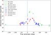 |
Fig. 6 Measured absolute R-band magnitudes of 324P in a 2300 km radius aperture plotted as a function of the true anomaly. The different symbols correspond to the different telescopes and instruments, and colors mark the perihelion passages: green for 2010, blue for 2015, and red for 2021. The vertical dashed line indicates perihelion. The horizontal dashed line corresponds to the absolute magnitude of the inactive nucleus (18.4 mag). |
3.3 Dependence of the aperture size on absolute dust magnitudes and Afρ
We now compare the time evolution of the magnitudes measured in differently sized apertures (Fig. 7). At ν = 45.7°, the brightness in the larger aperture (5″, black pentagons) has increased compared to earlier measurements, and the brightness in the smaller aperture (2300 km, green pentagons) has decreased. One possible cause of this discrepancy could be the changing geocentric distance, which affects the physical volume enclosed in an aperture with a fixed angular size. At Δ = 1.74 AU (ν = 18°), less volume is enclosed in the 5″ aperture than at 2.78 AU (ν = 45°), so that the absolute magnitude of dust in an aperture with a fixed angular size is expected to decrease with increasing distance to the observer. To better understand the dependence of the enclosed dust cross section on the aperture size and time, we calculated the A f ρ parameter (Table 3 and Fig. 8), which for a coma in steady state that is spherically symmetric is expected to be independent of the aperture size. A f ρ is the product of the albedo A, defined as the total light reflected by the cometary grains over the total light received, the filling factor f of the grains in the field of view, and ρ, the physical radius of the field of view (Fink & Rubin 2012). We used (A’Hearn et al. 1984)
![Mathematical equation: $\[A f \rho=\frac{\left(2 r_h \Delta\right)^2}{\rho} 10^{0.4\left(m_{\odot, R}-m_R\right)},\]$](/articles/aa/full_html/2024/10/aa51090-24/aa51090-24-eq10.png) (7)
(7)
where rh is the heliocentric distance in AU, Δ is the geocentric distance in cm, ρ is the physical radius in cm at the distance of the MBC, m⊙,R = −27.15 is the apparent R-band magnitude of the Sun, and mR is the measured apparent R-band magnitude of the MBC.
Plotting A f ρ versus true anomaly (Fig. 8, Panel A), we find that at ν = 45.7°, A f ρ is similar from both apertures (5″, and 2300 km). This behavior is consistent with a steady-state coma, and the difference of >1 mag in Fig. 7 results from the spatially extended nature of the dust coma, where larger apertures enclose more dust.
At true anomalies 12.8° and 18.4°, A f ρ increases with decreasing aperture size, indicating that the dust density decreases more steeply with increasing nucleus distance than in steady state. During this early phase of the activity, the dust production rate might still have been increasing with time, such that freshly emitted dust located close to the nucleus would be relatively more abundant than dust emitted at an earlier stage that had traveled farther at the time of observation. Hence, A f ρ derived from the smaller aperture would be higher.
However, the A f ρ parameter has some limitations: It assumes that there is no dust production or destruction (e.g., by fragmentation or sublimation of embedded ice) after the dust particles leave the nucleus, it assumes that the dust has a constant outflow velocity, and it fails at the turnaround distance (Fink & Rubin 2012). In panel B of Fig. 8, we plot A f ρ versus the aperture radius ρ at four epochs. The plot again shows a decrease in A f ρ with aperture size when 324P was freshly active in August and September 2010, a more shallow profile at the end of December 2010, and a flat, almost zero profile in August.
The flattening of the A f ρ profile at sufficiently large aperture radii during the first two epochs may suggest that during an even earlier epoch, the coma was closer to a steady-state regime than at the times of observation. This is consistent with Fig. 6, which shows a flat profile of absolute coma magnitudes up to a true anomaly of about 20° and then a steep increase.
In panel B of Fig. 8, at large ρ, the A f ρ parameter exhibits strong fluctuations that are likely due to an increasingly variable background flux as the aperture size increases. However, these fluctuations occur only beyond aperture radii of 5″ and are therefore not expected to significantly affect our interpretation of panel A of Fig. 8.
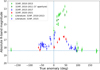 |
Fig. 7 Same as Fig. 6, but augmented by values from the literature (2010–2013: Hsieh et al. 2012b; Hsieh 2014, 2015: Hsieh & Sheppard 2015;Jewitt et al. 2016). Symbols now distinguish between our analysis of archival data and data from the literature (see legend). Pentagons with black edges were measured by us using a 5″ aperture for comparison with Hsieh et al. (2012b) (green crosses). |
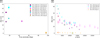 |
Fig. 8 A f ρ parameter. Panel A: A f ρ vs. true anomaly for 324P, evaluated using circular apertures with a physical radius of 2300 km (symbols without borders) and circular apertures with angular radius 5″ (symbols with black borders). Panel B: A f ρ vs. aperture radius ρ. The data enclosed by red circles correspond to the border-less symbols of panel A (ρ= 2300 km), and data enclosed by green squares correspond to the black-bordered data points of panel A (angular radius of 5″). |
A f ρ parameter.
3.4 Dust-mass estimates and onset of activity
We estimated the dust mass inside the aperture using (e.g. Hsieh & Sheppard 2015)
![Mathematical equation: $\[M_d=\frac{4}{3} \pi r_N^2 a \rho_d\left(\frac{1-10^{0.4\left(H_R-H_{R, {inactive}}\right)}}{10^{0.4\left(H_R-H_{R, {inactive}}\right)}}\right),\]$](/articles/aa/full_html/2024/10/aa51090-24/aa51090-24-eq11.png) (8)
(8)
where rN = 0.52 km is the estimated effective nucleus radius for 324P (Sec. 3.1), a = 1 mm is the assumed effective mean dust grain radius, ρd ~ 2500 kg m−3 is the assumed dust grain density (C-type objects), and HR,inactive = (18.4 ± 0.5) mag is the absolute magnitude of the inactive nucleus of 324P in the R band (Sect. 3.1). We plot our estimated dust masses as a function of the true anomaly in Fig. 9. The graphic shows that the MBC starts to be active near perihelion, and this suggests that the activity is due to sublimation. In Table A.1, we list the results of the photometric analysis. Three dust-mass values are negative but still consistent with zero, given the uncertainties.
Using a linear fit to the absolute magnitude as a function of time, Hsieh & Sheppard (2015) found the average net dust production rate ![Mathematical equation: $\[\left(\dot{M}_d\right)\]$](/articles/aa/full_html/2024/10/aa51090-24/aa51090-24-eq12.png) in 2015 for 324P to be ≲0.1 kg s−1 (−60.4° < ν < −41.4°), which is lower by almost 2 orders of magnitude than the net dust production rate value of ~30 kg s−1 (12.9° < ν< 45.9°) measured in 2010 by Hsieh (2014). These dust production rates from the literature were measured at different points in the orbit and were measured with rectangular apertures, aiming to capture the total visible flux (including coma and tail).
in 2015 for 324P to be ≲0.1 kg s−1 (−60.4° < ν < −41.4°), which is lower by almost 2 orders of magnitude than the net dust production rate value of ~30 kg s−1 (12.9° < ν< 45.9°) measured in 2010 by Hsieh (2014). These dust production rates from the literature were measured at different points in the orbit and were measured with rectangular apertures, aiming to capture the total visible flux (including coma and tail).
In our study, however, this linear fitting approach was not applicable because we observed nearly constant values in our dust measurements (Fig. 10). When we assume that dust particles are ejected from 324P with a speed comparable to the nucleus gravitational escape speed of υescape = 0.61 m s−1 (derived with the estimated nucleus size and assumed bulk density), they leave the 2300 km aperture after 43 days.
The data points displayed in Fig. 10 were collected over a period of several hundred days, suggesting that the earliest ejected dust had already left the measurement aperture at most epochs. Consequently, the nearly constant dust mass suggests that the rate of dust production from 324P may be roughly equal to the rate of dust loss from the aperture.
For the 2015 perihelion, we infer that the onset of activity took place earlier than 173 days before perihelion, when the image in Fig. A.1 shows a visible tail on 2015 June 10 (marked in Fig. 10). From the same criterion, we cannot infer anything about the onset time for the 2021 perihelion passage because no tail is visible in Fig. A.1 in the 2020 data.
In Fig. 7, near ν = 120°, the absolute magnitude stabilizes around 18.4 mag in the R band, consistent with our derived magnitude of the inactive nucleus (Sec. 3.1). This indicates that the dust production has ceased and that dust has left the immediate environment of the nucleus due to solar radiation pressure (in 2011).
Fig. 7 shows a steep increase in brightness at about and immediately after perihelion. To find the onset time of this steepening, we fit post-perihelion dust masses with a linear function. We determined the onset times of the profile steepening to be (33–81) days before perihelion in 2010 with a mass-loss rate of (5.5 ± 1.4) kg s−1 (0.0° < ν < 18.4°), 6 days before perihelion in 2015 with a mass-loss rate of (10 ± 4) kg s−1 (1.8° < ν < 4.5°), and between 23 days before perihelion and 8 days after perihelion in 2021 with a mass-loss rate of (0.9 ± 0.3) kg s−1 (1.0° < ν < 23.4°) (Fig. 11). This steep rise in activity is likely reflected in the A f ρ-profiles as discussed in Section 3.3. It may be caused by the thermal wave reaching a subsurface layer with elevated ice content, or by seasonal exposure of an ice reservoir that is not reached by sunlight before perihelion.
Hui & Jewitt (2017) studied data from 2010 to 2015 that indicated that 324P exhibited nongravitational accelerations caused by recoil forces due to anisotropic mass loss, with dynamically inferred mass-loss rates of (36 ± 3) kg s−1. This value agrees with the findings of Hsieh (2014) in 2010. However, our analysis of the 2010 data reveals mass-loss rates that differ by nearly an order of magnitude, which we discussed in Sec. 3.2 as possibly resulting from advances in all-sky photometric catalogs. Additionally, our estimated mass-loss rate agrees with that reported by Moreno et al. (2011), who found a value of 3–4 kg s−1 between 2010 October and 2011 January (26.5° < ν < 47.8°).
Figs. 7 and 9 visually confirm that the activity during the 2015 perihelion passage significantly decreased compared to the previous perihelion passage in 2010. The activity in 2021 also decreased compared to 2015.
A possible interpretation of the decrease in activity from one perihelion passage to the next may be given by the buildup of a dry mantle. Globally, ice-rich main-belt asteroids are thought to have a rubble mantle-type crust. Following the trigger event, the freshly exposed ice in an MBC sublimates and causes the observable activity. Dust particles that are too large to be ejected by the gas drag against gravity would accumulate on the surface. Gradually, this layer of dust and pebbles again becomes thick enough to act as a protective layer and buries the ice in the depths (Thiel et al. 1989; Jewitt 1992, 1996). In this scenario, the activity in MBCs should initially decrease rapidly after the trigger event. Subsequently, as a rubble mantle of sufficient thickness forms, the activity should decrease more slowly (Jewitt 1996; Hsieh et al. 2015, 2018a). This might be a possible explanation for the rapid decrease in the activity of 324P in 2015 compared to that in 2010 and the following slow decrease of its activity in 2021. Data from upcoming perihelia are required to corroborate this hypothesis, however.
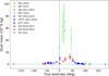 |
Fig. 9 Estimated dust masses for 324P plotted as a function of the true anomaly. The different symbols correspond to the different telescopes and instruments used, and the different colors correspond to the three different perihelion passages: green for 2010, blue for 2015, and red for 2021. The horizontal dashed line corresponds to a zero dust mass (the MBC was not active). |
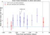 |
Fig. 10 Estimated dust masses around 324P plotted vs. time from perihelion. Pre-perihelion data in 2015 (blue) and pre- and post-perihelion data in 2021 (red). The epoch when the tail starts to become visible is marked in the plot. |
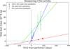 |
Fig. 11 Estimated dust masses around 324P plotted vs. time from perihelion. The dashed lines show linear fits to post-perihelion data from 2010 (green), 2015 (blue) and 2021 (red), which were used to calculate the time at which the activity increased. |
3.5 Analysis of infrared data
Thermal and scattered components
Infrared images provide information about the thermal emission from the grains (Sarmecanic et al. 1997), while visual images provide information about the reflectivity of the grains (Kolokolova et al. 2004). By combining these pieces of information, we calculated the geometric albedo of the cometary grains, which is defined as the ratio of the amount of light that is scattered by the grains to the amount of light that would be scattered to zero phase angle by a perfectly reflective, isotropic surface, known as a Lambertian surface (Hanner et al. 1981).
The thermal component is described by (Jewitt & Meech 1988)
![Mathematical equation: $\[F_{I R}=\frac{\varepsilon S B_\nu(T)}{\Delta^2},\]$](/articles/aa/full_html/2024/10/aa51090-24/aa51090-24-eq13.png) (9)
(9)
where FIR is the thermal flux density from the aperture in W m−2 Hz−1, ϵ is the emissivity, assumed here to equal unity, S is the cross section of the cometary grains inside the aperture in m2, Bv(T) is the Planck function evaluated at the temperature T in W m−2 Hz−1 sr−1, and Δ is the geocentric distance in meters.
The scattered component is given by (Russell 1916)
![Mathematical equation: $\[F_{\mathrm{vis}}=F_{\odot} \frac{p ~j(\alpha) S}{\left(r_h / 1 ~\mathrm{AU}\right)^2 \pi \Delta^2},\]$](/articles/aa/full_html/2024/10/aa51090-24/aa51090-24-eq14.png) (10)
(10)
where F⊙ is the solar spectrum at 1 AU and at the wavelength used for the measurement of the flux from the MBC, Fvis, and both are in the same units. The quantity p is the geometric albedo of the dust particles, j(α) is the scattering phase function, and rh and Δ are the heliocentric and geocentric distances in meters, respectively.
The spectral energy distribution (SED; Williams et al. 1997; Kolokolova et al. 2004; Yang et al. 2009) is composed of the superposition of scattered sunlight and thermal emission by the dust (Fig. 12). From the shape of the thermal SED, we first derived the dust temperature, then the product of dust cross section and emissivity, and the scattered component finally gives the product of geometric albedo and phase function divided by the emissivity at the time of observation of the cometary grains.
We derived the dust color temperature from equating the flux ratio in the WISE W4/W3 bands to the ratio of the Planck function at these wavelengths, Bv(22 μm, T) / Bv(12 μm, T), with the temperature Tcol as a free parameter, and obtained ![Mathematical equation: $\[T_{\text {col }}=167_{-11}^{+13} \mathrm{~K}\]$](/articles/aa/full_html/2024/10/aa51090-24/aa51090-24-eq15.png) . This temperature range includes the equilibrium temperature of a fast-rotating sphere with an isothermal surface, Teq=172 K, at the heliocentric distance during the WISE observation rh = 2.623 AU, with
. This temperature range includes the equilibrium temperature of a fast-rotating sphere with an isothermal surface, Teq=172 K, at the heliocentric distance during the WISE observation rh = 2.623 AU, with
![Mathematical equation: $\[T_{e q}\left(r_h, A_B, \varepsilon\right)=278.8\left(\frac{1-A_B}{\varepsilon}\right)^{\frac{1}{4}} \frac{1}{\sqrt{r_h}},\]$](/articles/aa/full_html/2024/10/aa51090-24/aa51090-24-eq16.png) (11)
(11)
where AB is the Bond albedo, assumed to be 0, ϵ is the emissivity, assumed to be 1, and rh is the heliocentric distance in AU. We conclude that there is no strong indication that dust superheats at mid-infrared (mid-IR) wavelengths, which is consistent with compact or large particles, or both (Gehrz & Ney 1992), but that color temperatures up to 8% above Teq are consistent with the WISE measurement.
To fit the combined SED of scattered light and thermal emission to the PS1 and WISE data, we scaled the Planck function, Bv, with a freely variable factor fIR and the solar spectrum8 with an also freely variable factor fvis, such that their sum matches the measured fluxes.
From Eq. (9), the scaling factor (in units of sr) fIR is equal to
![Mathematical equation: $\[f_{I R}\left(T_{c o l}\right)=\frac{\varepsilon S\left(T~_{c o l}\right)}{\Delta^2}.\]$](/articles/aa/full_html/2024/10/aa51090-24/aa51090-24-eq17.png) (12)
(12)
The S implicitly depends on the color temperature for a given measured flux FIR because of the temperature dependence of Bv(T) in Eq. (9). From Eq. (10), the dimensionless scaling factor for the scattering component is equal to
![Mathematical equation: $\[f_{v i s}=\frac{p j(\alpha) S}{\left(r_h / 1 ~\mathrm{AU}\right)^2 \pi \Delta^2},\]$](/articles/aa/full_html/2024/10/aa51090-24/aa51090-24-eq18.png) (13)
(13)
such that
![Mathematical equation: $\[\frac{p ~j(\alpha)}{\varepsilon}=\pi\left(r_h / 1 ~\mathrm{AU}\right)^2 \frac{f_{v i s}}{f_{I R}},\]$](/articles/aa/full_html/2024/10/aa51090-24/aa51090-24-eq19.png) (14)
(14)
assuming that the amount of dust seen in paired images is the same, despite different PSF and/or aperture sizes and observation dates. The maximum scaling factor, ![Mathematical equation: $\[f_{I R}^{max}\]$](/articles/aa/full_html/2024/10/aa51090-24/aa51090-24-eq21.png) , is obtained for the minimum possible color temperature, and vice versa. The minimum and maximum values for fvis result from fitting the solar spectrum to the lower and upper bound of the PS1 measurement error bar. Inserting these into Eq. (14), we find
, is obtained for the minimum possible color temperature, and vice versa. The minimum and maximum values for fvis result from fitting the solar spectrum to the lower and upper bound of the PS1 measurement error bar. Inserting these into Eq. (14), we find ![Mathematical equation: $\[p j(\alpha)=0.03_{-0.02}^{+0.12}\]$](/articles/aa/full_html/2024/10/aa51090-24/aa51090-24-eq22.png) . This corresponds to 3% < p < 45% for a C-type (G = 0.15 ± 0.12) phase function, and 2% < p < 40% for an S-type (G = 0.25 ± 0.12). Since this range includes all typical values measured for both C- and S-types, we cannot meaningfully constrain the geometric albedo or the spectral type of the dust. These large errors in the albedo calculation are due to the wide range of temperatures consistent with the mid-IR data and to large uncertainties in the photometry at optical wavelengths.
. This corresponds to 3% < p < 45% for a C-type (G = 0.15 ± 0.12) phase function, and 2% < p < 40% for an S-type (G = 0.25 ± 0.12). Since this range includes all typical values measured for both C- and S-types, we cannot meaningfully constrain the geometric albedo or the spectral type of the dust. These large errors in the albedo calculation are due to the wide range of temperatures consistent with the mid-IR data and to large uncertainties in the photometry at optical wavelengths.
Fig. 12 shows the minimum and maximum geometric albedo SEDs derived from the WISE/PS1 dataset together with these data, and in addition, the Spitzer and the extrapolated HST data (flux values in Tables 4 and 5). The latter were obtained during a different perihelion passage, when the overall dust brightness was lower than in 2010 (see Fig. 7), and from a different observer distance, but at very similar heliocentric distance, phase angle, and true anomaly. We show all six data points in a single graph because (1) the similar visible-light fluxes from PS1 and HST indicate that the overall amount of dust, scaled with Δ2, during both measurements was similar, (2) the similar heliocentric distances indicate that the color temperature range during both measurements was likely similar, and (3) the comparison with the WISE SEDs can give us some directions for the interpretation of the Spitzer data.
The plot shows that the longer of the two IRAC wavelengths lies in the overlapping zone where both scattered light and thermal emission can contribute significantly to the overall flux, while the flux measured at the shorter wavelength is most certainly dominated by scattered light, such that an independent measurement of the color temperature from the IRAC data is not possible. The dust brightness in the 4.5 μm IRAC measurement is also inconsistent with our simple model of representing the thermal emission by a single blackbody function. A possible cause for the elevated flux at 4.5 μm could be superheating because small or porous dust particles may not be able to thermally radiate efficiently at shorter wavelengths. Excess brightness in the IRAC 4.5 μm band has also been interpreted as an indicator for the presence of CO or CO2 vapor (Ootsubo et al. 2011), which we cannot exclude. However, our measured ratio of F(4.5 μm/3.6 μm) = 1.8 at rh = 2.625 AU is near the lower limit measured in 23 comets by Reach et al. (2013), where a low value of this ratio correlates with the absence of PSF broadening attributable to a spatially extended gas coma. We found no indications of an extended coma either, which again does not support the interpretation of our 4.5 μm excess flux as due to CO or CO2 emission. Depletion of CO2 relative to water was also observed in the MBC 238P by JWST (Kelley et al. 2023).
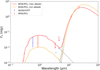 |
Fig. 12 SEDs corresponding to the maximum (red) and minimum (yellow) derived geometric albedo values from the WISE/PS1 combination. The Spitzer/HST data are also plotted (blue). Even though taken during different perihelion passages and from different observer distances, we plot the measurements and resulting fits in a single graph. The dashed lines indicate the pure blackbody and solar spectra composing the overall SED. |
Telescope and band of observation for the Spitzer/HST combination.
Telescope and band of observation for the WISE/PS1 combination.
4 Summary
We analyzed archival data of the MBC 324P in the period 2010–2021. We list our main results below:
Using only photometry measured when the MBC was observed to be inactive, we find the best-fit IAU phase function parameter HR = (18.4 ± 0.5) mag using G = 0.15 ± 0.12;
We calculated the effective nucleus radius, finding a value of rN = (0.52 ± 0.16) km (assuming geometric albedo pR = 0.05 ± 0.02);
We observed a decrease in its activity during the 2015 and 2021 perihelion passages compared to the previous passage in 2010. This decrease in the activity strength might be due to mantling and/or volatile depletion;
The study of the A f ρ profile and the absolute magnitudes of the dust coma across different true anomalies uncovered evidence that the coma of 324P transitioned near perihelion from a pre-perihelion steady state to a higher-activity post-perihelion steady state. This might indicate that a thermal wave arrived at more ice-rich layers, or it might indicate seasonal effects;
The study of the IR data yielded a dust geometric albedo in the range of (2–45)%, with unclear spectral type, but it suggested excess radiation at 4.5 μm in comparison to a single-temperature blackbody spectrum.
Further observations are necessary to monitor the future activity to constrain the possible causes for the decrease in the activity of 324P over time. On 2026 October 14, 324P will be at perihelion, and this may provide opportunities to gather further observations, data, and results. Furthermore, a data analysis of 324P during its inactive phases might enhance the accuracy of the IAU phase-function fitting. This might lead to an improved precision in determining absolute magnitudes and dust masses.
Acknowledgements
We thank the anonymous referee for their constructive input. We thank David Jewitt for his feedback on the manuscript, and the WISE Help Desk and the Pan-STARRS1 Help Desk for the support and information exchanged via mail. MM, YK and JA were funded by VolkswagenStiftung. The Pan-STARRS1 Surveys (PS1) and the PS1 public science archive have been made possible through contributions by the Institute for Astronomy, the University of Hawaii, the Pan-STARRS Project Office, the Max-Planck Society and its participating institutes, the Max Planck Institute for Astronomy, Heidelberg and the Max Planck Institute for Extraterrestrial Physics, Garching, The Johns Hopkins University, Durham University, the University of Edinburgh, the Queen’s University Belfast, the Harvard-Smithsonian Center for Astrophysics, the Las Cumbres Observatory Global Telescope Network Incorporated, the National Central University of Taiwan, the Space Telescope Science Institute, the National Aeronautics and Space Administration under Grant No. NNX08AR22G issued through the Planetary Science Division of the NASA Science Mission Directorate, the National Science Foundation Grant No. AST-1238877, the University of Maryland, Eotvos Lorand University (ELTE), the Los Alamos National Laboratory, and the Gordon and Betty Moore Foundation. PanSTARRS image identifiers: skycell.1760.023, skycell.1926.046, skycell.1926.047, skycell.1925.047. Based on observations made with the Isaac Newton Telescope under Director’s Discretionary Time of Spain’s Instituto de Astrofísica de Canarias. INT program: I/2010B/P14 (PI: Hsieh). Based on observations obtained at the international Gemini Observatory, a program of NSF’s NOIRLab (acquired through the Gemini Observatory Archive at NSF’s NOIRLab and processed using DRAGONS (Data Reduction for Astronomy from Gemini Observatory North and South)), which is managed by the Association of Universities for Research in Astronomy (AURA) under a cooperative agreement with the National Science Foundation on behalf of the Gemini Observatory partnership: the National Science Foundation (United States), National Research Council (Canada), Agencia Nacional de Investigación y Desarrollo (Chile), Ministerio de Ciencia, Tecnología e Innovación (Argentina), Ministério da Ciência, Tecnologia, Inovações e Comunicações (Brazil), and Korea Astronomy and Space Science Institute (Republic of Korea). Program IDs: GN-2011B-Q-17, GN-2013A-Q-102, GN-2016B-LP-11, GN-2020B-LP-104, GN-2021A-LP-104, GN-2021B-LP-104 and GS-2021B-LP-104 (PI: Hsieh). Based on observations made with the New Technology Telescope (NTT) at the ESO La Silla Observatory under the ESO program identifications 184.C-1143(E) and 184.C-1143(G) (PI: Hainaut). Based on observations collected at the European Organisation for Astronomical Research in the Southern Hemisphere (processed using EsoRex (ESO Recipe Execution Tool)) under ESO program identification 095.C-0932(A) (PI: Hsieh). Based on observations obtained with MegaPrime/MegaCam, a joint project of CFHT and CEA/DAPNIA, at the Canada-France-Hawaii Telescope (CFHT), which is operated by the National Research Council (NRC) of Canada, the Institut National des Science de l’Univers of the Centre National de la Recherche Scientifique (CNRS) of France, and the University of Hawaii. The observations at the Canada-France-Hawaii Telescope were performed with care and respect from the summit of Maunakea which is a significant cultural and historic site. Proposal IDs: 15AT05, 15BT12, 16AT06 and 16BT05 (PI: Hsieh). These results made use of the Lowell Discovery Telescope (LDT) at Lowell Observatory. Lowell is a private, nonprofit institution dedicated to astrophysical research and public appreciation of astronomy and operates the LDT in partnership with Boston University, the University of Maryland, the University of Toledo, Northern Arizona University and Yale University. The Large Monolithic Imager was built by Lowell Observatory using funds provided by the National Science Foundation (AST-1005313). Program ID: L02 (PI: Knight). We acknowledge Matthew M. Knight for providing the LDT images used in this study. This research is based on observations made with the NASA/ESA Hubble Space Telescope obtained from the Space Telescope Science Institute, which is operated by the Association of Universities for Research in Astronomy, Inc., under NASA contract NAS 5-26555. These observations are associated with programs 14263 and 14458 (PI: Jewitt). This publication makes use of data products from the Wide-field Infrared Survey Explorer, which is a joint project of the University of California, Los Angeles, and the Jet Propulsion Laboratory/California Institute of Technology, funded by the National Aeronautics and Space Administration. Scan IDs: 05353b, 05357b, 05361b, 05365b, 05369b, 05372a, 05373b, 05376a, 05377b, 05380a, 05381b, 05384a, 05388a, 05392a, 05396a, 05400a. This work is based in part on observations made with the Spitzer Space Telescope, which was operated by the Jet Propulsion Laboratory, California Institute of Technology under a contract with NASA. Program ID: 12043 (PI: Mommert). This research used the facilities of the Canadian Astronomy Data Centre operated by the National Research Council of Canada with the support of the Canadian Space Agency. This research has made use of the NASA/IPAC Infrared Science Archive, which is funded by the National Aeronautics and Space Administration and operated by the California Institute of Technology. This publication makes use of data products from the Near-Earth Object Wide-field Infrared Survey Explorer (NEOWISE), which is a joint project of the Jet Propulsion Laboratory/California Institute of Technology and the University of Arizona. NEOWISE is funded by the National Aeronautics and Space Administration. This research has made use of the software IRAF. IRAF is distributed by the National Optical Astronomy Observatories, which is operated by the Association of Universities for Research in Astronomy, Inc. (AURA) under cooperative agreement with the National Science Foundation. This research has made use of NASA’s Astrophysics Data System Bibliographic Services, JPL/Horizons ephemerides service, SAOImageDS9 application, and Python programming language.
Appendix A Figure and table
In this appendix, Fig A.1 and Table A.1 are provided.
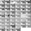 |
Fig. A.1 Mosaic of the visible-light images of 324P (at the center of each panel). All images are in the R band, except for two PS1 images on 2010 June 26 in the z band, and on 2010 September 8 in the g band. All panels show the north (N), the east (E), the antisolar direction (−⊙) and the negative heliocentric velocity vector (−υ), as projected on the sky. Panels are labeled with dates of observation in UT YYYY-MM-DD format, and employed telescope. The label PS1 refers to the Panoramic Survey Telescope and Rapid Response System PanSTARRS (PS1) telescope, equipped with the GPC1 instrument; INT to the Isaac Newton Telescope, equipped with the WFC instrument; GN to the Gemini Multi-Object Spectrograph North, equipped with the Gemini Multi-Object Spectrograph North (GMOS-N) instrument; NTT to the New Technology Telescope, equipped with the ESO Faint Object Spectrograph and Camera (EFOSC) instrument; VLT to the Very Large Telescope, equipped with the FOcal Reducer and low dispersion Spectrograph 2 (FORS2) instrument; CFHT to the Canada-France-Hawaii Telescope, equipped with the MegaPrime instrument; LDT to the Lowell Discovery Telescope, equipped with the Large Monolithic Images (LMI) instrument; and GS to the Gemini Multi-Object Spectrograph South, equipped with the Gemini Multi-Object Spectrograph South (GMOS-S) instrument. |
Observations of the MBC 324P.
References
- A’Hearn, M. F., Schleicher, D. G., Millis, R. L., Feldman, P. D., & Thompson, D. T. 1984, AJ, 89, 579 [Google Scholar]
- Bauer, J. M., Mainzer, A. K., Grav, T., et al. 2012, ApJ, 747, 49 [NASA ADS] [CrossRef] [Google Scholar]
- Bodewits, D., Kelley, M. S., Li, J.-Y., et al. 2011, ApJ, 733, L3 [NASA ADS] [CrossRef] [Google Scholar]
- Bowell, E., Hapke, B., Domingue, D., et al. 1989, in Asteroids II, Proceedings of the Conference,, eds. R. P. Binzel, T. Gehrels, & M. S. Matthews (Tuscon: University of Arizona Press) 524 [Google Scholar]
- Capria, M. T., Marchi, S., De Sanctis, M. C., Coradini, A., & Ammannito, E. 2012, A&A, 537, A71 [NASA ADS] [CrossRef] [EDP Sciences] [Google Scholar]
- Cutri, R. M., Wright, E. L., Conrow, T., et al. 2012, Explanatory Supplement to the WISE All-Sky Data Release Products [Google Scholar]
- Divine, N. 1981, in ESA Special Publication, 174, The Comet Halley. Dust and Gas Environment, eds. B. Battrick, & E. Swallow, 47 [Google Scholar]
- Drahus, M., Waniak, W., Tendulkar, S., et al. 2015, ApJ, 802, L8 [NASA ADS] [CrossRef] [Google Scholar]
- Fanale, F. P., & Salvail, J. R. 1989, Icarus, 82, 97 [NASA ADS] [CrossRef] [Google Scholar]
- Fazio, G. G., Hora, J. L., Allen, L. E., et al. 2004, ApJS, 154, 10 [Google Scholar]
- Fink, U., & Rubin, M. 2012, Icarus, 221, 721 [NASA ADS] [CrossRef] [Google Scholar]
- Gehrz, R., & Ney, E. 1992, Icarus, 100, 162 [CrossRef] [Google Scholar]
- Gwyn, S. D. J., Hill, N., & Kavelaars, J. J. 2012, PASP, 124, 579 [NASA ADS] [CrossRef] [Google Scholar]
- Haghighipour, N. 2009, Proc. Int. Astron. Union, 5, 207 [NASA ADS] [CrossRef] [Google Scholar]
- Haghighipour, N., Maindl, T. I., Schäfer, C., Speith, R., & Dvorak, R. 2016, ApJ, 830, 22 [CrossRef] [Google Scholar]
- Haghighipour, N., Maindl, T. I., Schäfer, C. M., & Wandel, O. J. 2018, ApJ, 855, 60 [NASA ADS] [CrossRef] [Google Scholar]
- Hanner, M. S., Giese, R. H., Weiss, K., & Zerull, R. 1981, A&A, 104, 42 [NASA ADS] [Google Scholar]
- Holmberg, J., Flynn, C., & Portinari, L. 2006, MNRAS, 367, 449 [NASA ADS] [CrossRef] [Google Scholar]
- Hsieh, H. H. 2014, Icarus, 243, 16 [CrossRef] [Google Scholar]
- Hsieh, H. H. 2015, Proc. Int. Astron. Union, 10, 99 [CrossRef] [Google Scholar]
- Hsieh, H. H., & Haghighipour, N. 2016, Icarus, 277, 19 [NASA ADS] [CrossRef] [Google Scholar]
- Hsieh, H. H., & Jewitt, D. 2006, Science, 312, 561 [NASA ADS] [CrossRef] [Google Scholar]
- Hsieh, H. H., & Sheppard, S. S. 2015, MNRAS, 454, L81 [CrossRef] [Google Scholar]
- Hsieh, H. H., Jewitt, D. C., & Fernández, Y. R. 2004, AJ, 127, 2997 [NASA ADS] [CrossRef] [Google Scholar]
- Hsieh, H. H., Jewitt, D., & Ishiguro, M. 2008, AJ, 137, 157 [Google Scholar]
- Hsieh, H. H., Jewitt, D., & Fernández, Y. R. 2009, ApJ, 694, L111 [NASA ADS] [CrossRef] [Google Scholar]
- Hsieh, H. H., Jewitt, D., Lacerda, P., Lowry, S. C., & Snodgrass, C. 2010, MNRAS, 403, 363 [NASA ADS] [CrossRef] [Google Scholar]
- Hsieh, H. H., Ishiguro, M., Lacerda, P., & Jewitt, D. 2011, AJ, 142, 29 [Google Scholar]
- Hsieh, H. H., Yang, B., Haghighipour, N., et al. 2012a, ApJ, 748, L15 [NASA ADS] [CrossRef] [Google Scholar]
- Hsieh, H. H., Yang, B., Haghighipour, N., et al. 2012b, AJ, 143, 104 [NASA ADS] [CrossRef] [Google Scholar]
- Hsieh, H. H., Denneau, L., Wainscoat, R. J., et al. 2015, Icarus, 248, 289 [NASA ADS] [CrossRef] [Google Scholar]
- Hsieh, H. H., Ishiguro, M., Kim, Y., et al. 2018a, AJ, 156, 223 [NASA ADS] [CrossRef] [Google Scholar]
- Hsieh, H. H., Novaković, B., Kim, Y., & Brasser, R. 2018b, AJ, 155, 96 [NASA ADS] [CrossRef] [Google Scholar]
- Hsieh, H. H., Micheli, M., Kelley, M. S. P., et al. 2023, Planet. Sci., 4, 43 [NASA ADS] [CrossRef] [Google Scholar]
- Hui, M.-T., & Jewitt, D. 2017, AJ, 153, 80 [NASA ADS] [CrossRef] [Google Scholar]
- IRAC Instrument and Instrument Support Teams 2021, IRAC Instrument Handbook [Google Scholar]
- Irwin, M., & Lewis, J. 2001, New A Rev., 45, 105 [NASA ADS] [CrossRef] [Google Scholar]
- Ishiguro, M., Hanayama, H., Hasegawa, S., et al. 2011, ApJ, 741, L24 [NASA ADS] [CrossRef] [Google Scholar]
- Jewitt, D. 1996, Earth Moon Planets, 72, 185 [NASA ADS] [CrossRef] [Google Scholar]
- Jewitt, D. 1992, Observations and Physical Properties of Small Solar System Bodies, Proceedings of the Liege International Astrophysical Colloquium, 30, 85 [NASA ADS] [Google Scholar]
- Jewitt, D., & Meech, K. J. 1988, AJ, 96, 1723 [CrossRef] [Google Scholar]
- Jewitt, D., Yang, B., & Haghighipour, N. 2009, AJ, 137, 4313 [NASA ADS] [CrossRef] [Google Scholar]
- Jewitt, D., Weaver, H., Mutchler, M., Larson, S., & Agarwal, J. 2011, ApJ, 733, L4 [NASA ADS] [CrossRef] [Google Scholar]
- Jewitt, D., Agarwal, J., Weaver, H., Mutchler, M., & Larson, S. 2013, ApJ, 778, L21 [NASA ADS] [CrossRef] [Google Scholar]
- Jewitt, D., Agarwal, J., Li, J., et al. 2014a, ApJ, 784, L8 [NASA ADS] [CrossRef] [Google Scholar]
- Jewitt, D., Ishiguro, M., Weaver, H., et al. 2014b, AJ, 147, 117 [NASA ADS] [CrossRef] [Google Scholar]
- Jewitt, D., Hsieh, H., & Agarwal, J. 2015, in Asteroids IV (University of Arizona Press) [Google Scholar]
- Jewitt, D., Agarwal, J., Weaver, H., et al. 2016, AJ, 152, 77 [NASA ADS] [CrossRef] [Google Scholar]
- Juan Luis Cano Rodríguez & Jorge Martínez Garrido 2022, in Proceedings of the 21st Python in Science Conference, eds. M. Agarwal, C. Calloway, D. Niederhut, & D. Shupe, 136 [Google Scholar]
- Kelley, M. S. P., Hsieh, H. H., Bodewits, D., et al. 2023, Nature, 619, 720 [NASA ADS] [CrossRef] [Google Scholar]
- Kim, Y., Ishiguro, M., & Lee, M. G. 2017a, ApJ, 842, L23 [NASA ADS] [CrossRef] [Google Scholar]
- Kim, Y., Ishiguro, M., Michikami, T., & Nakamura, A. M. 2017b, AJ, 153, 228 [NASA ADS] [CrossRef] [Google Scholar]
- Kim, Y., Agarwal, J., Jewitt, D., et al. 2022, A&A, 666, A163 [NASA ADS] [CrossRef] [EDP Sciences] [Google Scholar]
- Kolokolova, L., Hanner, M. S., Levasseur-Regourd, A.-C., Gustafson, B. A. S., & Binzel, R. P. 2004, Physical Properties of Cometary Dust from Light Scattering and Thermal Emission (University of Arizona Press), 577 [Google Scholar]
- Küppers, M., O’Rourke, L., Bockelée-Morvan, D., et al. 2014, Nature, 505, 525 [CrossRef] [Google Scholar]
- Lagerkvist, C. I., & Magnusson, P. 1990, A&AS, 86, 119 [Google Scholar]
- Magnier, E. 2006, in The Advanced Maui Optical and Space Surveillance Technologies Conference, E50 [Google Scholar]
- Magnier, E. A., & Cuillandre, J. C. 2004, PASP, 116, 449 [NASA ADS] [CrossRef] [Google Scholar]
- Mainzer, A., Grav, T., Masiero, J., et al. 2011, ApJ, 736, 100 [Google Scholar]
- Marinelli, M., & Dressel, L. 2024, Wide Field Camera 3 Instrument Handbook, Version 16.0 (Baltimore, MD: Space Telescope Science Institute) [Google Scholar]
- Masiero, J. R., Mainzer, A. K., Grav, T., et al. 2011, ApJ, 741, 68 [Google Scholar]
- Moreno, F., Lara, L. M., Licandro, J., et al. 2011, ApJ, 738, L16 [NASA ADS] [CrossRef] [Google Scholar]
- Moreno, F., Cabrera-Lavers, A., Vaduvescu, O., Licandro, J., & Pozuelos, F. 2013, ApJ, 770, L30 [NASA ADS] [CrossRef] [Google Scholar]
- Nomen, J., Birtwhistle, P., Holmes, R., Foglia, S., & Scotti, J. V. 2010, Central Bureau Electronic Telegrams, 2459, 1 [NASA ADS] [Google Scholar]
- Ootsubo, T., Kawakita, H., Hamada, S., et al. 2011, in EPSC-DPS Joint Meeting 2011, 369 [Google Scholar]
- Polishook, D., & Brosch, N. 2009, Icarus, 199, 319 [NASA ADS] [CrossRef] [Google Scholar]
- Pozuelos, F. J., Cabrera-Lavers, A., Licandro, J., & Moreno, F. 2015, ApJ, 806, 102 [NASA ADS] [CrossRef] [Google Scholar]
- Prialnik, D., & Rosenberg, E. D. 2009, MNRAS, 399, L79 [NASA ADS] [CrossRef] [Google Scholar]
- Reach, W. T., Kelley, M. S., & Vaubaillon, J. 2013, Icarus, 226, 777 [CrossRef] [Google Scholar]
- Russell, H. N. 1916, ApJ, 43, 173 [Google Scholar]
- Sarmecanic, J., Fomenkova, M., Jones, B., & Lavezzi, T. 1997, ApJ, 483, L69 [NASA ADS] [CrossRef] [Google Scholar]
- Schleicher, D. 2010, Composite Dust Phase Function for Comets, https://asteroid.lowell.edu/comet/dustphase/, Accessed: July 3, 2024 [Google Scholar]
- Schorghofer, N. 2008, ApJ, 682, 697 [NASA ADS] [CrossRef] [Google Scholar]
- Schorghofer, N. 2016, Icarus, 276, 88 [NASA ADS] [CrossRef] [Google Scholar]
- Schörghofer, N., & Hsieh, H. H. 2018, J. Geophys. Res. (Planets), 123, 2322 [CrossRef] [Google Scholar]
- Sheppard, S. S., & Trujillo, C. 2015, AJ, 149, 44 [NASA ADS] [CrossRef] [Google Scholar]
- Thiel, K., Koelzer, G., Kochan, H., et al. 1989, In ESA, Physics and Mechanics of Cometary Materials, 302, 221 [NASA ADS] [Google Scholar]
- Tody, D. 1986, SPIE Conf. Ser., 627, 733 [Google Scholar]
- Tody, D. 1993, in Astronomical Society of the Pacific Conference Series, 52, Astronomical Data Analysis Software and Systems II, eds. R. J. Hanisch, R. J. V. Brissenden, & J. Barnes, 173 [Google Scholar]
- Tonry, J. L., Stubbs, C. W., Lykke, K. R., et al. 2012, ApJ, 750, 99 [Google Scholar]
- Williams, D. M., Mason, C. G., Gehrz, R. D., et al. 1997, ApJ, 489, L91 [NASA ADS] [CrossRef] [Google Scholar]
- Willmer, C. N. A. 2018, ApJS, 236, 47 [Google Scholar]
- Wright, E. L., Eisenhardt, P. R. M., Mainzer, A. K., et al. 2010, AJ, 140, 1868 [Google Scholar]
- Yang, B., Jewitt, D., & Bus, S. J. 2009, AJ, 137, 4538 [NASA ADS] [CrossRef] [Google Scholar]
ETC Request IDs: WFC3UVIS.im.1845086, WFC3UVIS.im. 1845087, WFC3UVIS.im.1845088, WFC3UVIS.im.1845089.
ETC Request IDs: WFC3UVIS.im.1843958, WFC3UVIS.im.1843962.
https://www.nrel.gov/grid/solar-resource/spectra.html, F⊙, the Thekaekara Spectrum.
All Tables
All Figures
|
Fig. 1 Orbit plot in the heliocentric ecliptic coordinate system. The origin is the center of the Sun, the plane of reference is the ecliptic plane, and the direction of the x-axis points toward the vernal equinox. The plot shows the positions of 324P at the epochs of our observations with the orbits of Mercury, Venus, Earth, Mars, 324P, and Jupiter. Crosses represent the perihelion (P) and aphelion (A) positions. Pentagons, triangles, squares and circles represent visual data, and diamonds and stars are IR data. (The plot was generated using the poliastro Python library; Juan Luis Cano Rodríguez & Jorge Martínez Garrido 2022.) |
| In the text | |
|
Fig. 2 IR images of 324P (at the center of each panel). The label W3 refers to WISE band 3 (12 μm), W4 to WISE band 4 (22 μm), and IRAC1 and IRAC2 corresponds to Spitzer Space Telescope observations at 3.6 μm and 4.5 μm, respectively. The dates and directions on sky are labeled as in Fig. A.1. |
| In the text | |
|
Fig. 3 Visual-light images (PS1 in the z band and HST in the V band) of 324P (at the center of each panel). The dates and directions on sky are labeled as in Fig. A.1. These visual images were obtained closest in time to the respective IR images shown in Fig. 2. |
| In the text | |
|
Fig. 4 Absolute V-band magnitudes of 324P plotted as a function of the true anomaly and linear fit for extrapolation. The blue dots show HST measurements, and the red dot shows the extrapolated value for 2016 January 8. The central solid line represents the fit to the data, and the dashed lines parallel to the solid line represent the uncertainty of the linear fit. |
| In the text | |
|
Fig. 5 Best-fit IAU phase function (solid red line) for 324P. The dashed red lines represent the uncertainty of the fit. The blue points show 2013 data, when the nucleus was inactive. These were used for the fit. |
| In the text | |
|
Fig. 6 Measured absolute R-band magnitudes of 324P in a 2300 km radius aperture plotted as a function of the true anomaly. The different symbols correspond to the different telescopes and instruments, and colors mark the perihelion passages: green for 2010, blue for 2015, and red for 2021. The vertical dashed line indicates perihelion. The horizontal dashed line corresponds to the absolute magnitude of the inactive nucleus (18.4 mag). |
| In the text | |
|
Fig. 7 Same as Fig. 6, but augmented by values from the literature (2010–2013: Hsieh et al. 2012b; Hsieh 2014, 2015: Hsieh & Sheppard 2015;Jewitt et al. 2016). Symbols now distinguish between our analysis of archival data and data from the literature (see legend). Pentagons with black edges were measured by us using a 5″ aperture for comparison with Hsieh et al. (2012b) (green crosses). |
| In the text | |
|
Fig. 8 A f ρ parameter. Panel A: A f ρ vs. true anomaly for 324P, evaluated using circular apertures with a physical radius of 2300 km (symbols without borders) and circular apertures with angular radius 5″ (symbols with black borders). Panel B: A f ρ vs. aperture radius ρ. The data enclosed by red circles correspond to the border-less symbols of panel A (ρ= 2300 km), and data enclosed by green squares correspond to the black-bordered data points of panel A (angular radius of 5″). |
| In the text | |
|
Fig. 9 Estimated dust masses for 324P plotted as a function of the true anomaly. The different symbols correspond to the different telescopes and instruments used, and the different colors correspond to the three different perihelion passages: green for 2010, blue for 2015, and red for 2021. The horizontal dashed line corresponds to a zero dust mass (the MBC was not active). |
| In the text | |
|
Fig. 10 Estimated dust masses around 324P plotted vs. time from perihelion. Pre-perihelion data in 2015 (blue) and pre- and post-perihelion data in 2021 (red). The epoch when the tail starts to become visible is marked in the plot. |
| In the text | |
|
Fig. 11 Estimated dust masses around 324P plotted vs. time from perihelion. The dashed lines show linear fits to post-perihelion data from 2010 (green), 2015 (blue) and 2021 (red), which were used to calculate the time at which the activity increased. |
| In the text | |
|
Fig. 12 SEDs corresponding to the maximum (red) and minimum (yellow) derived geometric albedo values from the WISE/PS1 combination. The Spitzer/HST data are also plotted (blue). Even though taken during different perihelion passages and from different observer distances, we plot the measurements and resulting fits in a single graph. The dashed lines indicate the pure blackbody and solar spectra composing the overall SED. |
| In the text | |
|
Fig. A.1 Mosaic of the visible-light images of 324P (at the center of each panel). All images are in the R band, except for two PS1 images on 2010 June 26 in the z band, and on 2010 September 8 in the g band. All panels show the north (N), the east (E), the antisolar direction (−⊙) and the negative heliocentric velocity vector (−υ), as projected on the sky. Panels are labeled with dates of observation in UT YYYY-MM-DD format, and employed telescope. The label PS1 refers to the Panoramic Survey Telescope and Rapid Response System PanSTARRS (PS1) telescope, equipped with the GPC1 instrument; INT to the Isaac Newton Telescope, equipped with the WFC instrument; GN to the Gemini Multi-Object Spectrograph North, equipped with the Gemini Multi-Object Spectrograph North (GMOS-N) instrument; NTT to the New Technology Telescope, equipped with the ESO Faint Object Spectrograph and Camera (EFOSC) instrument; VLT to the Very Large Telescope, equipped with the FOcal Reducer and low dispersion Spectrograph 2 (FORS2) instrument; CFHT to the Canada-France-Hawaii Telescope, equipped with the MegaPrime instrument; LDT to the Lowell Discovery Telescope, equipped with the Large Monolithic Images (LMI) instrument; and GS to the Gemini Multi-Object Spectrograph South, equipped with the Gemini Multi-Object Spectrograph South (GMOS-S) instrument. |
| In the text | |
Current usage metrics show cumulative count of Article Views (full-text article views including HTML views, PDF and ePub downloads, according to the available data) and Abstracts Views on Vision4Press platform.
Data correspond to usage on the plateform after 2015. The current usage metrics is available 48-96 hours after online publication and is updated daily on week days.
Initial download of the metrics may take a while.