| Issue |
A&A
Volume 628, August 2019
|
|
|---|---|---|
| Article Number | A92 | |
| Number of page(s) | 21 | |
| Section | Extragalactic astronomy | |
| DOI | https://doi.org/10.1051/0004-6361/201935832 | |
| Published online | 12 August 2019 | |
Constraining nuclear star cluster formation using MUSE-AO observations of the early-type galaxy FCC 47⋆
1
European Southern Observatory, Karl Schwarzschild Straße 2, 85748 Garching bei München, Germany
e-mail: This email address is being protected from spambots. You need JavaScript enabled to view it.
2
Department of Astrophysics, University of Vienna, Türkenschanzstrasse 17, 1180 Wien, Austria
3
Max-Planck-Institut für Astronomie, Königstuhl 17, 69117 Heidelberg, Germany
4
University of California Santa Cruz, 1156 High Street, Santa Cruz, CA 95064, USA
5
Shanghai Astronomical Observatory, Chinese Academy of Sciences, 80 Nandan Road, Shanghai 200030, PR China
6
Dipartimento di Fisica e Astronomia “G. Galilei”, Università di Padova, Vicolo dell’Osservatorio 3, 35122 Padova, Italy
7
INAF–Osservatorio Astronomico di Padova, Vicolo dell’Osservatorio 5, 35122 Padova, Italy
8
Instituto de Astrofísica de Canarias, Calle Via Láctea s/n, 38200 La Laguna, Tenerife, Spain
9
Depto. Astrofísica, Universidad de La Laguna, Calle Astrofísico Francisco Sánchez s/n, 38206 La Laguna, Tenerife, Spain
10
INAF-Astronomical Observatory of Capodimonte, Via Moiariello 16, 80131 Napoli, Italy
11
Department of Physics and Astronomy, Macquarie University, North Ryde, NSW 2109, Australia
12
Armagh Observatory and Planetarium, College Hill, Armagh BT61 9DG, UK
13
Centre for Astrophysics Research, University of Hertfordshire, College Lane, Hatfield AL10 9AB, UK
14
Sterrewacht Leiden, Leiden University, Postbus 9513, 2300 RA Leiden, The Netherlands
15
Max-Planck-Institut für Extraterrestrische Physik, Gießenbachstraße 1, 85748 Garching bei München, Germany
Received:
3
May
2019
Accepted:
28
June
2019
Abstract
Context. Nuclear star clusters (NSCs) are found in at least 70% of all galaxies, but their formation path is still unclear. In the most common scenarios, NSCs form in-situ from the galaxy’s central gas reservoir, through the merging of globular clusters (GCs), or through a combination of both.
Aims. As the scenarios pose different expectations for angular momentum and stellar population properties of the NSC in comparison to the host galaxy and the GC system, it is necessary to characterise the stellar light, NSC, and GCs simultaneously. The large NSC (reff = 66 pc) and rich GC system of the early-type Fornax cluster galaxy FCC 47 (NGC 1336) render this galaxy an ideal laboratory to constrain NSC formation.
Methods. Using Multi Unit Spectroscopic Explorer science verification data assisted by adaptive optics, we obtained maps for the stellar kinematics and stellar-population properties of FCC 47. We extracted the spectra of the central NSC and determined line-of-sight velocities of 24 GCs and metallicities of five.
Results. The galaxy shows the following kinematically decoupled components (KDCs): a disk and a NSC. Our orbit-based dynamical Schwarzschild model revealed that the NSC is a distinct kinematic feature and it constitutes the peak of metallicity and old ages in FCC 47. The main body consists of two counter-rotating populations and is dominated by a more metal-poor population. The GC system is bimodal with a dominant metal-poor population and the total GC system mass is ∼17% of the NSC mass (∼7 × 10⁸ M⊙).
Conclusions. The rotation, high metallicity, and high mass of the NSC cannot be explained by GC-inspiral alone. It most likely requires additional, quickly quenched, in-situ formation. The presence of two KDCs likely are evidence of a major merger that has significantly altered the structure of FCC 47, indicating the important role of galaxy mergers in forming the complex kinematics in the galaxy-NSC system.
Key words: galaxies: individual: NGC 1336 / galaxies: nuclei / galaxies: kinematics and dynamics / galaxies: star clusters: general
Based on observation collected at the ESO Paranal La Silla Observatory, Chile, Prog. ID 60.A-9192, PI Fahrion.
© ESO 2019
1. Introduction
The nuclei of galaxies are extreme environments located at the bottom of the galactic potential well, in which numerous complex astrophysical processes take place and various phenomena occur such as active galactic nuclei caused by accretion onto supermassive black holes (SMBHs), central star bursts, and extreme stellar densities. As the properties of a galactic nucleus are related to properties of the host galaxy (e.g. Magorrian et al. 1998; Kormendy & Ho 2013), the evolution of nucleus and host seems to be closely linked. Thus, understanding the origin of physical properties of the nucleus gives insight into galaxy evolution. Traditionally, the relations between the mass of the SMBH and host galaxy properties were explored. Subsequently, nuclear star clusters (NSCs) were included in these relations to extend them to lower masses of the central massive object (e.g. Ferrarese et al. 2006; Graham & Driver 2007; Georgiev et al. 2016; Spengler et al. 2017; Ordenes-Briceño et al. 2018).
NSCs are dense stellar systems that reside in the photometric (Böker et al. 2002) and kinematic centre (Neumayer et al. 2011) of a galaxy, often co-existing with a central black hole (e.g. Seth et al. 2008a; Graham & Spitler 2009; Schödel et al. 2009; Neumayer & Walcher 2012; Georgiev et al. 2016). Typical NSCs have sizes similar to globular clusters (GCs, reff ∼ 5 − 10 pc, Böker et al. 2004; Côté et al. 2006; Turner et al. 2012; den Brok et al. 2014; Georgiev & Böker 2014; Puzia et al. 2014), but exhibit a broader mass range between 105 and 108 M⊙ (Walcher et al. 2005; Georgiev et al. 2016; Spengler et al. 2017). Their central stellar densities often reach extreme values, up to 105 M⊙ pc−3, (Hopkins et al. 2009), and are only comparable to the densities found in some GCs and ultra compact dwarf galaxies (UCDs, Hilker et al. 1999a; Drinkwater et al. 2000). Since especially the more massive UCDs are regarded as the nuclear remnants of stripped dwarf galaxies, it is not surprising that massive UCDs and NSCs have similar properties (e.g. Phillipps et al. 2001; Pfeffer & Baumgardt 2013; Strader et al. 2013; Norris et al. 2015).
NSCs are very common and can be found in 70% to 80% of all galaxies, from dwarf to giant galaxies of all morphologies (Böker et al. 2002; Côté et al. 2006; Georgiev et al. 2009; Eigenthaler et al. 2018). Sánchez-Janssen et al. (2019) found that the nucleation fraction reaches 90% for galaxies with M* ≈ 109 M⊙ and declines for both higher and lower masses. NSCs can show complex density distributions with flattening light profiles (Böker et al. 2002) and they can exhibit multiple stellar populations (Walcher et al. 2006; Lyubenova et al. 2013; Kacharov et al. 2018), sometimes having a significant contribution from young stellar populations (Rossa et al. 2006; Paudel et al. 2011). NSCs in early-type galaxies (ETGs) in the Virgo galaxy cluster were found to cover a broad range of metallicities (Paudel et al. 2011) and they are often more metal-rich than their host galaxy (Spengler et al. 2017). In addition, many NSCs have been observed to show significant rotation (Seth et al. 2008b, 2010; Lyubenova et al. 2013; Lyubenova & Tsatsi 2019), with the NSC of the Milky Way being the most prominent example (Feldmeier et al. 2014). As nuclear stellar disks usually have similar sizes to NSCs (Scorza & Bender 1995; Pizzella et al. 2002), it is possible that some NSCs are nuclear stellar disks seen face on.
There are several suggested formation scenarios for NSCs that distinguish between two main pathways. In the in-situ formation scenario, NSCs form directly at the galactic centre from infalling gas (Bekki et al. 2006; Bekki 2007; Antonini et al. 2015). This formation mode depends on internal feedback mechanisms and the available gas content (Mihos & Hernquist 1994; Schinnerer et al. 2008). Different mechanisms for funnelling gas to the centre have been studied, such as magnetorotational instability, gas cloud mergers, or instabilities from bar structures (Milosavljević 2004; Bekki 2007; Schinnerer et al. 2008). On the other hand, NSC formation might happen through gas-free accretion of GCs that have formed at larger galactic radii and migrate inwards due to dynamical friction (Tremaine et al. 1975; Capuzzo-Dolcetta 1993; Capuzzo-Dolcetta & Miocchi 2008; Agarwal & Milosavljević 2011; Arca-Sedda & Capuzzo-Dolcetta 2014). Also, the formation of nuclear stellar disks via this channel has been explored (Portaluri et al. 2013). While the pure in-situ scenario seems to be unable to reproduce some of the observed scaling relations between NSC and host (Antonini 2013), the dry merger scenario has been more successful in this respect (Arca-Sedda & Capuzzo-Dolcetta 2014; Hartmann et al. 2011).
Studies that have compared the predictions from simulations to observational data have shown that most likely both scenarios are realised in nature (Hartmann et al. 2011; Antonini et al. 2015) and propose that in-situ formation can contribute a large fraction (up to 80%) to the total NSC mass. Motivated by this, Guillard et al. (2016) proposed a composite “wet migration” scenario where a massive cluster forms in the early stages of galaxy evolution in a gas-rich disk and then migrates to the centre while keeping its initial gas reservoir, possibly followed by mergers with other gas-rich clusters.
The different formation scenarios impose different expectations on the properties of the NSC compared to the host galaxy and its GC system. In the in-situ scenario, the NSC forms independent of the GC system and one expects to see more rotation in the NSC due to gas accretion from a disk, and higher metallicities as a consequence of efficient star formation, and quick metal enrichment (e.g. Seth et al. 2006). The NSC can show an extended star formation history as a result from continuing gas accretion and episodic star formation. In the dry GC accretion scenario, the NSC should reflect the metallicity of the accreted GCs (Perets & Mastrobuono-Battisti 2014) and should show less strong rotation due to the random in-fall directions, however, simulations have shown that NSCs formed through GC mergers, in some cases, also can have significant rotation because they share the angular moment of their formation origin (Hartmann et al. 2011; Tsatsi et al. 2017). The kinematic and chemical properties of the surviving GC population can provide insight into the potential contributors to the NSC in this dry scenario. However, if the mergers of gas-rich or young star clusters is considered, studies have shown that these can result in a complex star formation history of the NSC (Antonini 2014; Guillard et al. 2016).
Constraining NSC formation observationally is therefore a complex issue and requires a panoramic view of the kinematic and chemical structure of the stellar body, the NSC, and GC population of a galaxy. This can be achieved with modern-day wide-field integral field unit (IFU) instruments as they allow a simultaneous observation a galaxy from its very centre to the halo and are able to spatially and spectrally resolve the different components.
The early-type galaxy FCC 47 (NGC 1336) in the outskirts of the Fornax galaxy cluster (rproj = 780 kpc to NGC 1399) at a heliocentric distance of 18.3 ± 0.6 Mpc (10″ ≈ 0.9 kpc, Blakeslee et al. 2009, see Fig. 1 and Table 1 for basic information about FCC 47) offers an ideal laboratory to explore NSC formation. Using the Hubble Space Telescope (HST) data from the ACS Fornax Cluster Survey (ACSFCS, Jordán et al. 2007), Turner et al. (2012) determined that FCC 47 has a particularly large NSC with an effective radius of reff = 0.750 ± 0.125″ = 66.5 ± 11.1 pc in the F475W filter (≈g-band, see also the surface brightness profile in Fig. 1). Jordán et al. (2015) identified more than 300 GC candidates associated with FCC 47. In the recent ACSFCS study of GC specific frequencies of Liu et al. (2019), FCC 47 appears as an outlier with a specific frequency SN, z = 4.61 ± 0.211 that is much higher than the typical (∼1) specific frequency of ETGs with similar mass. The NSC of FCC 47 was also studied with adaptive optics (AO)-supported high angular resolution integral-field spectroscopy (IFS) observations with the Spectrograph for INtegral Field Observations in the Near Infrared (SINFONI) by Lyubenova & Tsatsi (2019) among five other NSCs of ETGs in the Fornax cluster (see also Lyubenova et al. 2013). The NSC of FCC 47 stands out from this sample due to its large size, strong rotation and pronounced velocity dispersion peak.
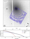 |
Fig. 1. Photometric HST/ACS data of FCC 47. Top: HST image of FCC 47 in the F475W filter (roughly g-band). Surface brightness contours from the collapsed MUSE cube (white light image) are superimposed in purple. The levels are logarithmically spaced, but arbitrarly chosen for illustration purposes. Bottom: surface brightness profile of FCC 47 in the F475W filter with a double Sersic profile fit, reproducing the plot from Turner et al. (2012). |
Basic information about FCC 47.
In this paper, we aim to constrain the formation of FCC 47’s massive NSC. We use observations with the Multi Unit Spectroscopic Explorer (MUSE) instrument that enables a simultaneous study of the kinematic and chemical properties of FCC 47’s stellar body, its NSC, and the GC system. In an accompanying paper (Fahrion et al. 2019), we report the discovery of a UCD in the MUSE field of view (FOV). Based on its size, magnitude and stellar mass, the UCD is consistent with being the remnant NSC of a stripped metal-poor dwarf galaxy with an initial mass of a few 108 M⊙, indicating that FCC 47 might have undergone a minor merger. However, its properties are also consistent with it being the most massive GC of FCC 47, although its large effective radius of 24 pc makes it an outlier with respect to other GCs.
We describe the MUSE data briefly in Sect. 2. We present the methods to extract MUSE spectra in Sect. 3 and how kinematic and stellar population properties were extracted in Sect. 4.1. The results of our kinematic analysis are presented in Sects. 5 and 6 gives the results for the stellar population analysis. Section 7 describes our Schwarzschild orbit-based model that was used to explore the origin of the dynamical structure of FCC 47. We discuss our findings in Sect. 8 and give our summary and conclusions in Sect. 9.
2. MUSE adaptive optics observations
The MUSE instrument provides the ideal means for our goals of studying the known large NSC and the rich GC system of FCC 47. MUSE is an integral-field spectrograph mounted at UT4 on the Very Large Telescope (VLT) in Paranal, Chile. Its wide field mode (WFM) provides a continuous FOV of 1′×1′ with a spatial sampling of 0.2″ and a spectral resolution of 2.5 Å (FWHM) at 7000 Å in an optical wavelength range between 4500 and 9300 Å.
Our data were acquired during the Science Verification (SV) phase (60.A-9192, P.I. Fahrion) in September 2017 after the commissioning of the Ground Atmospheric Layer Adaptive Corrector for Spectroscopic Imaging (GALACSI) AO system. We placed the NSC in a corner of the MUSE FOV (see Fig. 1). This off-centre positioning was chosen such that a simultaneous observation of the NSC as well as a large number of GCs was possible.
We designed our observation of FCC 47 following the observing strategy for the galaxies in the Fornax 3D survey (F3D, Sarzi et al. 2018). This survey targets bright galaxies within the virial radius of the Fornax cluster and uses deep MUSE observations to explore the formation and evolution of galaxies in a dense cluster environment. Like for the F3D galaxies, the exposures of FCC 47 were dithered by a few arcseconds and rotated by 90° to reduce the signature of MUSE’s 24 integral-field units on the final image. The data consist of ten exposures with 360 seconds exposure time each. Dedicated sky exposures of three minutes were taken in between the science exposures to perform sky modelling and reduce the contamination from sky emission lines. Our MUSE + AO data were taken in the nominal mode, meaning a wavelength coverage from 4750 to 9300 Å. In addition, the regime from 5800 to 6000 Å is filtered out because the AO facility works with four strong sodium lasers that would saturate the detector in the sodium D line (see Fig. 4).
Due to unfortunate weather conditions, the seeing during the observation was ∼1.6″, however, the AO system was able to reduce this to a final full width at half maximum (FWHM) of the point spread function (PSF) of ∼0.7″. The data are not ideal to study the effect of the AO system on the MUSE PSF as there is only one bright foreground star in the FOV that is located close to the centre of the galaxy. Its light profile therefore suffers from strong contamination from the bright galaxy background. Nonetheless, we fitted both a Gaussian and Moffat profile using IMFIT (Erwin 2015) and achieved equally good results. We therefore assumed a Gaussian PSF profile with a FWHM of 0.7″ needed for the extraction of GC spectra although the precise shape of the PSF is not crucial for our study. The PSF FWHM corresponds to the effective radius of the NSC in FCC 47 (also 0.7″), meaning that the especially large NSC allowed us to formally resolve it, while usually NSCs at this distance cannot be resolved with MUSE WFM.
We processed the raw data following the standard reduction pipeline version 2.2 (Weilbacher et al. 2014) incoporated in a ESO reflex environment (Freudling et al. 2013) that is able to handle the AO data. The data reduction includes bias and overscan subtraction, flat-field correction, wavelength calibration, determination of the line-spread function, and illumination correction. To further reduce the sky residual lines, we applied the Zurich Atmosphere Purge (ZAP) principal component analysis algorithm (Soto et al. 2016).
3. Extraction of spectra
In the following, we describe how we extract MUSE spectra from the different stellar components in FCC 47. We differentiate between the integrated galaxy light, the GCs, and the NSC.
3.1. Galaxy stellar light
The extraction of stellar light kinematics and especially stellar population properties requires a minimum spectral signal-to-noise ratio (S/N). To get a continuous view of these properties from the integrated stellar light, we binned the MUSE data with the Python version of the Voronoi binning routine described in Cappellari & Copin (2003). This method enables an adaptive binning to provide a constant spectral S/N per bin. We chose a target S/N of 100 Å−1 to ensure an accurate extraction of the line-of-sight velocity distribution (LOSVD) parameters as well as the metallicity, stellar age and α-element abundance. For the purpose of creating a reliable dynamical Schwarzschild orbit-superposition model, S/N = 100 is necessary (Krajnović et al. 2015). To avoid accreting large bins in the outer regions, where errors are strongly non-Poissonian, we excluded all spaxels with S/N < 1 Å−1. The Voronoi-binned MUSE cube contains 435 bins (see Fig. 5).
3.2. Globular clusters
To extract the spectra of GCs from the MUSE cube, we performed the following steps: First, their spatial location in the unbinned MUSE data was determined. This is difficult in the collapsed MUSE image as the majority of GCs (among other point sources) are hidden in the high surface brightness area of the galaxy. For this reason, we determined the individual GC positions after subtracting a model of the galaxy creating a residual image in which the point sources can be identified with standard peak-finding methods. While this has been commonly done in photometric studies, here we had the extra fidelity and luxury of being able to identify the residual signatures of GCs in each single wavelength slice of the MUSE data cube. To ensure a sufficient spatial S/N for the detection of GCs, we created residual images of different slabs from the blue to the red end of the data cube, each containing 50 combined wavelength slices. It is also possible to create a full residual data cube that can be used, for example, to easily identify astrophysical objects with emission lines, such as planetary nebulae or background star-formation galaxies. In the case of FCC 47, we used such a residual cube to identify three background galaxies (see Fig. 3).
A variety of different approaches were tested to create residual images including a simple unsharp mask approach using a median filter, Multi-Gaussian expansion (MGE, Bendinelli 1991; Monnet et al. 1992; Emsellem et al. 1994; Cappellari 2002) modelling and a multi-component IMFIT model (Erwin 2015). The unsharp mask approach has to be used carefully to avoid losing the faintest GCs and sources in the bright central region. Using MGE or IMFIT yielded consistent results, but for reasons of time efficiency, we use a simple MGE model using the code described in Cappellari (2002). However, for other galaxies that have a more complex morphology (e.g. disks with bulges), MGE modelling might be insufficient for removing the galaxy light and IMFIT should be used in these cases.
After the MGE model was subtracted from the image, point sources were extracted using DAOSTARFINDER, a Python module that implements the DAOPHOT algorithm (Stetson 1987) into a Python class. This code is usually used to find real point sources like stars, but also detects slightly extended sources very well. DAOSTARFINDER returns a list of image coordinates of point sources, but these are not exclusively GCs. A contamination from unresolved background galaxies and foreground stars has to be considered. We used the ancillary catalogue of GC candidates from the ACSFCS (Jordán et al. 2015) for cross-reference and to build the inital sample of GC candidates. The candidates in this cataloguewere selected based on their photometric and morphological characteristics, following the approach described in Jordán et al. (2007).
We detected 43 GC candidates from the HST catalogue out of 93 in that region and used the associated positional information to extract their spectra from the MUSE cube. We used a PSF-weighted circular aperture extraction assuming a Gaussian PSF with FWHM = 0.7″ (3.5 pixels) on the original data cube. Because many of the GC candidates are in high surface brightness areas, we also extracted and subtracted a background spectrum from an annulus aperture around each GC candidate to characterise the local galaxy contribution. The annulus had a width of 5 pixel and the inner radius was placed 8 pixels from the GC centre. The background spectrum was averaged over the used pixels to normalise for the area and no further scaling is applied. For GCs closer than 10″ from the galaxy centre we chose an aperture width of 3 pixels and a distance of 6 pixels because of the more strongly varying background. For GCs with distances larger than 30″, we use annuli with a width of 9 pixels to ensure a high S/N background spectrum. However, for these outer GCs, the background level is low (see surface brightness profile in Fig. 1). The annulus size was chosen to optimise the S/N of the final background-subtracted GC spectrum. Choosing a size that differs by only a few pixels does not affect the recovered radial velocities and mean metallicites considerably, but can increase the uncertainties by a few percent.
Inspecting the GC spectra, we found one GC candidate close in projection to the NSC that is not a GC, but rather a star-forming background galaxy at redshift z ∼ 0.34 with visible emission lines of hydrogen, nitrogen and oxygen. In addition to this object, we found two other background galaxies with strong emission lines in the MUSE cube as shown in Fig. 3.
The top panel in Fig. 2 shows a histogram of all GC g-band magnitudes from ACSFCS in comparison to the ones that were found in the MUSE data. It reveals that our sample is complete down to a g-band magnitude of 23 mag. We are missing five GCs with a magnitude of < 24 mag because they all lie within 10″ in projection from the galaxy centre. In this central region, the extraction of GCs is difficult due to the strongly varying galaxy background that is not completely removed by our MGE model, as the residuals show (Fig. 3). The bottom panel of Fig. 2 shows the histogram of spectral S/N of the extracted GCs, determined in a continuum region around 6500 Å. We find 25 GCs with S/N > 3, out of those 17 have S/N > 5 Å−1 and 5 GCs even reach S/N > 10 Å−1. A S/N > 3 is required to measure a reliable line-of-sight (LOS) velocity (see Appendix A) and to confirm membership to the FCC 47 systems. The remaining candidates cannot be confirmed as GCs due to their low S/N. With our approach we found 42 of 93 (45%) GC candidates from the ACSFCS catalogue in the MUSE FOV. The detection of GCs with MUSE strongly depends on the PSF FWHM.
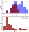 |
Fig. 2. Distributions of magnitudes and S/N of the extracted GCs. Top: distribution of g-band magnitudes of the GC candidates in the MUSE FOV from Jordán et al. (2015) (blue). The red distribution highlights the GC candidates found in the MUSE data with our method. Bottom: histogram of spectral S/N of the GC candidates and FCC 47-UCD1. |
In addition to the GC candidates that were already in the catalogue, it is possible to add sources manually by inspecting their spectra. We reported the discovery of a UCD with a spectral S/N ∼ 20 Å−1 in an accompanying paper (Fahrion et al. 2019, see also Fig. 3). We included FCC 47-UCD1 in the analysis of the GCs presented below, but highlight it as a distinct object in the associated figures.
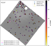 |
Fig. 3. Residual image of FCC 47 after subtracting a MGE model of the galaxy. The coloured crosses show the position of GC candidates in the HST catalogue of Jordán et al. (2015), colour-coded by their g-band magnitude. The black circles show the position of 42 GC candidates that are found with the DAOSTARFINDER routine in the MUSE data by cross referencing with the catalogue. The diamond indicates the position of FCC 47-UCD1 with a g-band magnitude of ∼21 mag. The triangles indicate the positions of emission-line background galaxies we found in the MUSE cube. |
3.3. Spectrum of the nuclear star cluster
The exceptionally large size of the NSC in FCC 47 and its brightness allowed us to extract a MUSE spectrum of the NSC. The analysis from Turner et al. (2012) showed that the NSC dominates the inner ∼0.5″ by more than 2 mag. This implies that the inner few spaxels are completely dominated by the light of the NSC, however, there still is a non-negligible contribution from the underlying galaxy. To extract a clean NSC spectrum we used a similar approach as for the GC spectra and used a PSF-weighted circular aperture in combination with a annulus-extracted background spectrum. This approach treats the NSC as another point-source, although it is formally resolved within our MUSE data. Nonetheless, we chose the PSF-weighted extraction to maximise the flux from the NSC. The galaxy background was determined in an annulus aperture that is placed at 5 pixels separation from the central pixel and has a width of 3 pixels. This way, we determined the galaxy contribution directly outside of the NSC, which is crucial to estimate the flux level of the background that shows a strong gradient in the central region. We subtracted the background spectrum from PSF-weighted NSC spectrum both normalised to the same area without additional weighting, such that we assume that the background flux level is flat between the centre and the position where we extract the annulus spectrum. This is a justified assumption as for example the double Sérsic decomposition as presented in Turner et al. (2012) shows. From the position where we take the annulus spectrum to the centre, the galaxy component’s surface brightness varies by < 1 mag arcsec−2, but this depends on the two component Sérsic fit to the galaxy light profile. For reference, we show the local galaxy spectrum together with the background subtracted NSC spectrum in Fig. 4. The galaxy background is clearly bluer than the NSC and thus applying an additional weight to it in the subtraction would result in a even redder NSC spectrum. The background-subtracted NSC spectrum has a spectral S/N ∼ 125 Å−1.
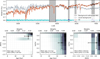 |
Fig. 4. PPXF fit to the background subtracted NSC spectrum. Top: original normalised spectrum is shown in black, the best-fit spectrum in red. For comparison, the spectrum of the local galaxy background is shown in grey. The residual is shown in blue, shifted to 0.6 for visualisation. Masked regions appear as grey shaded. We masked strong sky line residuals as well as the empty region around the sodium D line that is filtered out due to the AO lasers. Bottom: weight maps illustrating the age – metallicity (left), age – [α/Fe] (middle) and [α/Fe] – metallicity (right) grids. The weight of each template used in the fit is given by the greyscale. The black cross shows the weighted mean age, metallicity and α-element abundance with errorbars. The weight maps are normalised. A regularisation parameter of 30 was used in this fit. |
4. Extracting kinematics and stellar population properties
The following sections describe how we extract kinematics and stellar population properties from the extracted MUSE spectra. Again, we differentiate between galaxy light, NSC, and GCs.
4.1. Fitting with PPXF
We used the penalised Pixel-fitting (PPXF) method (Cappellari & Emsellem 2004; Cappellari 2017) to extract the stellar kinematics and population properties, such as mass-weighted mean ages and metallicities, from the MUSE spectra. PPXF is a full-spectrum fitting method that uses a penalised maximum likelihood approach to fit a combination of user-provided template spectra to the target spectrum. We chose the single stellar population (SSP) template spectra from the Medium resolution INT Library of Empirical Spectra (MILES, Vazdekis et al. 2010). These SSP synthesis models give the spectral energy distributions for stellar populations of a single age and single metallicity. The original MILES spectra have a coverage between 3525 and 7500 Å. The extended library, called E-MILES, covers a broader wavelength range from 1680 to 50 000 Å including the spectral lines of the Calcium Triplet around 8500 Å. The template spectra in both libraries have a spectral resolution of 2.5 Å (Falcón-Barroso et al. 2011), the mean instrumental resolution of MUSE. We use the description of the line spread function from Guérou et al. (2016; see also Emsellem et al. 2019). Throughout this work, we use BaSTI isochrones (Pietrinferni et al. 2004, 2006) and a Milky Way-like, double power law (bimodal), inital mass function (IMF) with a high mass slope of 1.30 (Vazdekis et al. 1996).
Although the E-MILES templates allow us to fully exploit the broad wavelength coverage of the MUSE instrument, only so-called “baseFe” models are available. These reproduce the metallicity and light element abundance pattern of the Milky Way and assume [M/H]=[Fe/H] for high metallicities. For lower metallicities, α-enhanced input spectra are used, such that [M/H] is higher than [Fe/H] (Vazdekis et al. 2010). On the other hand, the MILES models have a restricted wavelength range, but additionally offer scaled solar models ([α/Fe] = 0) and alpha enhanced models ([α/Fe] = 0.4 dex). These α-variable MILES models allow to study the distribution of α-abundances from high S/N spectra. Because the original MILES library only offers two different [α/Fe] values, using a regularised fit with PPXF seems unphysical. To create a better sampled grid of SSP models for the fits, we linearly interpolated between the available SSPs to create a grid from [α/Fe] = 0 to [α/Fe] = 0.4 dex with a spacing of 0.1 dex. These models were created under the assumption that the [α/Fe] abundances behave linearly in this regime and only give the average [α/Fe], however, in reality the abundances of different α-elements might be decoupled. The low S/N of the GC spectra make an extraction of [α/Fe] abundances challenging. We therefore fitted the GCs with the E-MILES SSP templates to exploit the broad wavelength range of these models, but we noted a metallicity offset of 0.2 dex between E-MILES and scaled solar MILES models. This is caused by the way the E-MILES templates are constructed to match the Milky Way abundance pattern: the input low-metallicity spectra are metal-enhanced (Vazdekis et al. 2016).
To summarise, we used the baseFe E-MILES templates for the GC spectra on the full MUSE wavelength range to determine estimates of the LOS velocity and metallicities. To extract ages, metallicities and [α/Fe] abundances from the high S/N spectra of the NSC and the integrated stellar light, we used the α-variable MILES spectra on a wavelength range from 4500 to 7100 Å.
We did not fit simultaneously for the kinematics and stellar population properties, but used a two-step approach (Sánchez-Blázquez et al. 2014). Each spectrum was first fitted for its LOSVD parameters using additive polynomials of order 25 and no multiplicative polynomials to ensure a well-behaved continuum that is necessary to get an accurate measurement of the LOSVD parameters. In the second step, the LOSVD parameters were fixed for the fit of the stellar population parameters and we used multiplicative polynomials of order eight instead of additive polynomials as the relative strength of absorption lines is crucial to determine the stellar population properties. In the end, the PPXF fit returned the LOSVD parameters and the weight coefficients of each input SSP template. In this way, the age and metallicity distributions can be recovered.
4.2. Galaxy light and NSC spectrum
The high S/N of the binned stellar light and the NSC spectrum allowed us to accurately measure the LOSVD parameters and recover the distribution of ages and metallicities. We fitted for the LOS velocity, the velocity dispersion and the higher order moments h3 and h4.
We estimated the typical uncertainties of the kinematic fit using a Monte Carlo (MC) approach (e.g. Cappellari & Emsellem 2004; Pinna et al. 2019). After the first fit, we drew randomly from the PPXF residual in each wavelength bin and added this to the (noise-free) best-fit spectrum to create 300 realisations that were fitted to obtain a well-sampled distribution. The uncertainty is then given by the standard deviation (or 16th and 84th percentile) of this distribution. Testing uncertainties in five different bins, we found maximum uncertainties of 4 km s−1 and 6 km s−1 for the stellar LOS velocity and velocity dispersion, respectively. For the higher moments of the LOSVD, h3 and h4, we found typical uncertainties of 0.02 km s−1 for both.
By construction, using SSP templates discretises the stellar population distribution of a galaxy. Regularisation can be used to find a smooth solution by enforcing smooth variations from one weight to its neighbours. This is especially crucial for the recovery of star formation histories from the data. Finding the right regularization parameter is, however, non-trivial (see e.g, Boecker et al. 2019). Typically, the regularization parameter is determined on a sub-sample of spectra and then kept fixed (as described in McDermid et al. 2015). We calibrated the regularization on a few binned spectra taken from the central part of the galaxy following the recommendation by Cappellari (2017) and McDermid et al. (2015): Firstly, the noise spectrum is rescaled to obtain a unit χ2 in an unregularised fit. Then, the regularization parameter is given by the one that increases the χ2 value of the fit by  , where Npix is the number of fitted (unmasked) spectral pixels. This value gives the smoothest solution that is still consistent with the data. Based on this calibration, we used a regularisation parameter of 70 for the binned stellar light fits.
We treated the cleaned NSC spectrum similarly to the galaxy light spectra. It has a S/N of 125 Å−1 that allows to extract age, metallicities and [α/Fe] distributions. Because of this high S/N, we calibrated the regularisation separately and used a regularisation parameter of 30 for the PPXF fit. Figure 4 shows the fit to the cleaned NSC spectrum. The bottom panels of this figure show the grid of age, metallicity and [α/Fe] models. The best-fit model is the weighted sum of the SSPs with their weights colour-coded.
4.3. Globular clusters
In contrast to the stellar light, the GCs have a low S/N (< 20 Å−1). This prevented us from detailed stellar population analysis as especially the age is ill-constrained at this spectral quality, and fitting α-element abundances is even more challenging. In addition, the intrinsic velocity dispersion of typical GCs is ∼10 km s−1, well below the MUSE instrumental resolution and therefore not accessible. Nonetheless, bright GCs allowed us to determine their radial velocity and estimate their mean metallicity. We tested the requirements for the S/N as described in Appendix A and found that radial velocities can be recovered down to a S/N > 3 Å−1, whereas the mean metallicity can be estimated for S/N > 10 Å−1 under the assumption that the GCs are single stellar population objects. We used the E-MILES SSP templates to fit the GCs, because their broad wavelength range helps to reduce uncertainties.
Since the S/N varies strongly among the GCs, we determined the radial velocity (and, if possible the mean metallicity) with its uncertainty for each GC using 300 realisations in an MC-like fashion as described in Sect. 4.2. As we could not find indications of young ages (< 10 Gyr) in unrestricted fits, we restricted the SSP library to ages > 10 Gyr to speed up the MC runs for the velocity and metallicity measurements. In the best cases, the random uncertainties on the velocity and metallicity, determined from the width of the MC distribution, were < 10 km s−1 and ∼0.10 dex, respectively (see Table C.1). The afore mentioned regularisation approach can be used for high S/N spectra of the stellar light and the NSC. For the GCs, however, we assumed them to be SSP objects and do not use regularisation in the fit. The mean metallicity should be unaffected. As mentioned before, choosing the α-enhanced MILES models instead of the E-MILES causes a constant shift of ∼0.2 dex towards higher metallicities, while relative metallicities stay constant.
5. Kinematics
In the following, we describe our results of the extraction of kinematics from the MUSE spectra. We differentiate between the high S/N spectra of integrated galaxy light and the low S/N results from the GCs.
5.1. Galaxy light
The maps of stellar light LOS mean velocity v, velocity dispersion σ and the higher order LOSVD parameters h3 and h4 for FCC 47 are shown in Fig. 5. The velocity map revealed FCC 47’s interesting velocity structure. While there is no net rotation visible at larger radii in the FOV, a small rotating disk with a diameter of roughly 20″ (∼2 kpc) was found near the centre. This feature is rotating with a maximum velocity of ≲20 km s−1, relative to the systemic galaxy velocity of 1444.4 ± 2.0 km s−1. While this disk structure is rotating along the main photometric axis, the very centre of FCC 47 is rotating around a different axis offset by ∼115°. The NSC rotation is seen over an extent of ∼3″ (250 pc, 15 pixels).
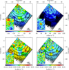 |
Fig. 5. Stellar light kinematic maps for FCC 47 acquired from the Voronoi-binned MUSE cube. Top left: mean relative velocity of the integrated light with respect to a systemic velocity of 1444 km s−1. Top right: velocity dispersion σ. Bottom left: h3 and bottom right: h4. The inset shows a zoom to the central region to highlight the inner structure. We show the same isophotes as used in Fig. 1. The effective radius of the NSC (0.7″) corresponds to the radius of the innermost isophote contour. |
The velocity dispersion map shows a strong peak in the centre, where it reaches values of ∼125 km s−1 and drops sharply to values of ∼80 km s−1 before showing a more gradual decrease to values < 60 km s−1 in the outskirts. The h3 and h4 maps are rather featureless, but h3 shows anti-correlation to the rotation of the disk structure.
The rotation in the centre matches the rotation of the NSC as studied by Lyubenova & Tsatsi (2019) using SINFONI+AO data. In the MUSE data, the NSC does not reach the same maximum velocity and velocity dispersion as in the SINFONI data. The maximum rotation velocity is reduced from ∼60 km s−1 observed with SINFONI down to ∼20 km s−1. Additionally, the velocity dispersion is less peaked in the MUSE data and only reaches 125 km s−1 instead of 160 km s−1 in the SINFONI data. By convolving the SINFONI maps to match the MUSE PSF with a Gaussian kernel, we found that this difference is caused by the larger MUSE PSF that smears out the NSC’s contribution to the velocity structure. This clear link between the SINFONI and MUSE structures shows, however, that the rotating central structure is indeed the NSC of FCC 47.
Both the rotating disk structure and the NSC classify as kinematically decoupled components (KDCs) because they are decoupled from the non-rotating main body of FCC 47. KDCs were discovered decades ago with long-slit spectroscopy (Efstathiou et al. 1982; Franx & Illingworth 1988). Large IFS surveys such as SAURON (Bacon et al. 2001) or ATLAS3D (Cappellari et al. 2011) have revealed that a significant fraction of ETGs have a KDC, especially slow-rotators (Emsellem et al. 2007). Simulations suggest that the formation of KDCs is triggered by major mergers (Jesseit et al. 2007; Bois et al. 2011; Tsatsi et al. 2015), but once formed, a KDC can be stable over a long time in a triaxial galaxy (van den Bosch et al. 2008; Rantala et al. 2019). KDCs are not rare in slow-rotating galaxies like FCC 47, however two decoupled components certainly are. To explore the nature and origin of FCC 47’s dynamical structure, we constructed an orbit-based dynamical Schwarzschild model (Sect. 7) based on the MUSE kinematic data.
Using the Wide Field Spectrograph (WiFeS, Dopita et al. 2010) on the Australian National University 2.3-m telescope, Scott et al. (2014) presented LOS velocity and velocity dispersion maps of FCC 47 among nine other ETGs in the Fornax clusters and classified FCC 47 as a fast rotator based on their data. However, we find that our MUSE maps do not resemble the WiFeS data at all. The reason for this is unknown.
5.2. Globular clusters
For the 25 GCs with S/N > 3 Å−1, we determined their radial velocities with PPXF (see Table C.1). We could not find any signs of rotation in the GC system due to our small sample size. Figure 6 shows the relative GC velocities with respect to the systemic velocity of FCC 47 as function of their projected distance from the galactic centre, colour-coded by their (g − z) colour from the ACSFCS catalogue (Jordán et al. 2015). The solid line gives the circular velocity amplitude for FCC 47 based on the results from our dynamical model (Sect. 7). FCC 47-UCD1 is shown as the diamond symbol. The green shaded area indicates the maximum visible rotation amplitude seen in the stellar light map and reveals that the radial velocities for many GCs do not exceed this amplitude, meaning that they are bound to FCC 47. This is particularly true for the red GC population (g − z > 1.15 mag) as they show less scatter around the systemic velocity of FCC 47, having a velocity dispersion of 23.0 ± 3.8 km s−1. The blue GCs, however, span a wider range of velocities and have a velocity dispersion of 42.0 ± 6.8 km s−1. The uncertainties refer to the uncertainties from fitting a Gaussian distribution to the histogram of LOS velocities.
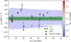 |
Fig. 6. Radial profile of LOS velocities of GCs in comparison to the observed scatter in stellar light velocities (green shaded area). The blue shaded area shows the circular velocity profile of FCC 47 as obtained from the orbit-based dynamical model (Sect. 7). The colour of the GCs and FCC 47-UCD1 refers to their (g − z) colour in AB magnitudes taken from Jordán et al. (2015). We show all GCs with S/N > 3 Å−1. The errorbars refer to the 1σ random uncertainty from fitting each GC 300 times. |
6. Stellar population properties
Besides kinematics, we also extracted stellar population properties from the MUSE spectra of the galaxy, the NSC, and the GCs. In the following we describe our results of the stellar population analysis.
6.1. Galaxy light
From the weights given by the regularised PPXF fit of the alpha-variable MILES SSP template spectra to the Voronoi binned data, we constructed maps of mean age, metallicity and alpha-element abundance ratios ([α/Fe]) as shown in Fig. 7. The centre of FCC 47 reaches super-solar metallicities and shows a strong gradient towards lower metallicities within 10″ from the centre. The outskirts reach a metallicity of ∼−0.4 dex. The extent of the metal-rich central region is the same as the rotating NSC seen in Fig. 5. As the comparison to SINFONI data showed, this region is completely dominated by the light from the NSC, smeared out by the MUSE PSF. The NSC appears to be significantly metal-richer than the surrounding galaxy. The shown maps were extracted using the α-variable MILES models, but we found a very similar metallicity distribution when using the baseFe E-MILES models, however, shifted to lower metallicities by 0.2 dex (see the metallicity gradient shown in Fig. 9). This is most likely caused by the rather smooth distribution of α-abundances in the outskirts, as the right panel in Fig. 7 illustrates. This is in contrast to the MW-like behaviour, encapsulated in the baseFe E-MILES models. The main body of FCC 47 is α-enhanced and shows lower values on the extent of the rotating disk structure. The NSC cannot be seen as a separate component in the [α/Fe] map, but shows similar values as the disk of [α/Fe] ∼ 0.25 dex.
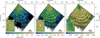 |
Fig. 7. Stellar population maps of FCC 47. Mean ages (left), metallicities [M/H] (middle) and [α/Fe] abundance ratios (right) as determined from a full spectrum fit with PPXF using the alpha-variable MILES template spectra. The maps are mass weighted. We show the same isophotes as in Fig. 1. The inset shows a zoom to the central region and the innermost isophote contour corresponds to the size of the NSC (Reff = 0.7″). |
FCC 47 is overall old (> 8 Gyr) with a gradient towards older ages in the centre and the NSC (∼13 Gyr). This is also reflected in the star formation histories (SFHs) shown in Fig. 8. We show the SFHs of the background-subtracted NSC, the central region (corresponding to the unsubtracted NSC), the disk structure, and the remaining galaxy body. These SFHs were mass-weighted and normalised by their integral. The central component was defined as all bins within 8 pixels (1.6″) around the centre. The disk component was described by an ellipse that traces the extent of the rotating disk structure and the galaxy component contains the remaining bins out to a semi major axis distance of 200 pixels (see Fig. 8). While the background-subtracted NSC is completely dominated by a single star formation peak at very old ages, the disk shows a smaller secondary peak at ∼8 Gyr. This secondary peak is visible in the central region, but the comparison to the clean NSC SFH shows that this is due to contamination from the galaxy and not attributed to the NSC itself. The outer galaxy seems to have formed last with the youngest ages found here and this region shows a broad peak in the SFH, centred at ∼8 Gyr. As the mean ages (dashed vertical lines) illustrate, FCC 47 has a very old centre and younger outskirts while the disk region shows a transition from old to younger ages and contains two separate populations.
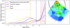 |
Fig. 8. Mass weighted, normalised star formation histories of different components of FCC 47. Left: background subtracted NSC in purple, central component in red, the disk in blue and the remaining stellar body in yellow. The dotted lines give the mean ages of each component. The normalisation is chosen such that the weights of each component add up to unity. Right: radial velocity map of FCC 47 as shown in Fig. 5. The black ellipses illustrate how we divided the different components. |
The mass fraction of the old stellar population (> 11 Gyr) decreases from 93% in the background-subtracted NSC to 79% in the centre to 48% in the disk to 20% in the rest of the galaxy. Using the same spatial decomposition, we found that the NSC is dominated by a metal-rich population ([M/H] > 0 dex) that constitutes 67% of the mass in both the cleaned NSC spectrum and the central region. This mass fraction reduces to 47% in the disk and to 29% in the outskirts. Comparing the different maps, we find that the metallicity shows a strong gradient of ∼0.5 dex between NSC and the effective radius of the galaxy (30″) and the mean age decreases from 13 Gyr to 9 Gyr over the same extent, while the [α/Fe] abundances show a much milder gradient and increase by ∼0.1 dex.
6.2. The nuclear star cluster
We fitted the background-subtracted NSC spectrum separately to the binned stellar light (see Fig. 4), allowing a detailed study of the NSC’s stellar populations. For comparison, we also show the spectrum of the local background that was used for the subtraction. This background spectrum is clearly bluer than the cleaned NSC spectrum and applying no subtraction would therefore bias the stellar population analysis towards younger ages or more metal-poor populations. From the weight maps shown (Fig. 4), we again found that the NSC shows little substructure in ages and thus must have formed very early on without any later episodes of star formation. However, we found indications of two separate populations that differ in metallicity: There seems to be a dominating metal-rich population and a secondary population with lower metallicities. The dominant metal-rich component constitutes 67% of the NSC mass. The two populations seem to have similar [α/Fe] values. We note, because our models only included [α/Fe] values from 0.0 to 0.4 dex, boundary effects from the model grid can introduce uncertainties, but the presence of two populations with different metallicities should be real.
The stellar population analysis allowed us to estimate the stellar mass of the NSC. As we did not have predictions for the mass-to-light ratio from the α-variable MILES models, we fitted the NSC again with the E-MILES SSP models and use their predictions for the stellar mass-to-light ratio for each age and metallicity in the HST/ACS F475W filter. The inferred age and metallicity weights were then translated into mass-to-light ratio weights. The weighted mean mass-to-light ratio of the NSC is 5.3 M⊙/L⊙. Varying [α/Fe] will have a small effect on the mass-to-light ratio, however, the uncertainty of the derived mass is governed by the uncertainty on the magnitude. Turner et al. (2012) found an apparent magnitude of the NSC of 16.09 ± 0.19 mag in the ACS F475W filter (g-band), translating to a luminosity of L = (1.37 ± 0.23)×108 L⊙, assuming a distance modulus of 31.31 mag (Blakeslee et al. 2009). For the photometric mass, we found MNSC, phot = (7.3 ± 1.2)×108 M⊙, corresponding to ∼5% of the total stellar mass of FCC 47. The uncertainty was inferred from 1000 draws assuming a Gaussian distribution of the magnitude. With this mass, the NSC of FCC 47 is among the more massive known NSCs as was already expected from its large size. The mass agrees with the enclosed mass profile from the dynamical model (see Fig. 12) within the inner 2.7″, the extent of the NSC in the MUSE data.
6.3. Globular clusters
Measuring the metallicities of the GCs is challenging due to the low S/N. As described in Appendix A, we found that PPXF gives reliable metallicity estimates for GCs with a S/N > 10 Å−1. The MUSE data enabled us to estimate spectroscopic metallicities for a sub-sample of 5 GCs and FCC 47-UCD1 (see Table C.1). For this measurement, we used the E-MILES SSP templates because they give the smallest uncertainty due to the broad wavelength range. As mentioned above, using scaled solar MILES templates results in similar metallicities, while the α-enhanced E-MILES models gave higher metallicities with a constant offset of 0.2 dex.
The metallicities of the five GCs and FCC 47-UCD1 are shown in a radial profile presented in Fig. 9. Four of those GCs have a blue colour and are metal-poor, while the fifth GC is red and metal-rich. Its metallicity is comparable to that of the NSC. Due to the low number of GCs with metallicity estimate, our view on FCC 47’s GC system is biased. We therefore show the radial (g − z) colour distribution from the ACSFCS for the GC candidates of FCC 47 in the bottom panel of Fig. 9. We show all GCs that have a probability of being a genuine GC pGC > 0.95. These are 205 GCs. The colours of the NSC (Turner et al. 2012) and FCC 47-UCD1 (Fahrion et al. 2019) are added and we mark the GCs with crosses for which we have spectroscopic metallicities. The radial distribution of GC colours also shows the red and blue subpopulations. The red GCs (g − z > 1.15 mag) are more centrally concentrated, which is also reflected in the running mean that shows a radial gradient of mean GC colours from red to blue.
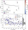 |
Fig. 9. Radial profile of GC metallicities in comparison to their photometric colours, the NSC, and the integrated galaxy light. Top: radial profile of the mean stellar metallicity (black line) with GCs (circles), UCD (diamond) and the NSC (star). The symbols are colour-coded by their (g − z) colours from Jordán et al. (2015) and Turner et al. (2012). Bottom: (g − z) colours of the photometric sample of GC candidates from Jordán et al. (2015) versus projected distance. The NSC and FCC 47-UCD1 are added and we mark the GCs for which we have spectroscopic metallicity measurements. The dotted line is the mean of GC colours in bins of 10 arcsec. The NSC colour is the colour within a 4-pixel aperture on the HST/ACS images (Turner et al. 2012). We also included the histogram of GC colours to illustrate the bimodal colour distribution. |
We used the photometric colours to determine the total mass of the GC system in a similar fashion to the mass of the NSC, however, mostly based on photometric SSP predictions that show an age-metallicity degeneracy. Under the assumption that all GCs have an age of 13 Gyr, we used the E-MILES SSP predictions for the HST/ACS filters to convert (g − z) colours to metallicities and subsequently to mass-to-light ratios. With the g-band magnitudes from the HST catalogue, these are then converted to photometric masses. This way, we estimate the total mass of the GC system (including FCC 47-UCD1 and all GCs with pGC > 0.5) to be ∼1.2 × 10⁸ M⊙. A mass fraction of 77% is in the blue GC population (g − z < 1.15 mag), 23% in the red. This estimate is not precise, but shows that the entire GC system only constitutes ∼17% of the mass found in the NSC (7 × 10⁸ M⊙), even though FCC 47 has a large GC system for its mass.
In massive ETGs, the mass of the GC system is often found to be proportional to the total stellar mass MGC = (1 − 5)×10−3 M* (Spitler & Forbes 2009; Georgiev et al. 2010; Harris et al. 2013). For FCC 47, this relation would imply a total GC system mass of (1.6 − 8.0)×107 M⊙. While the relation between GC system mass and stellar mass of a galaxy can show significant scatter, it has been established that the total GC system mass forms a near-linear relation with the total halo mass of a galaxy (Spitler & Forbes 2009; Georgiev et al. 2010; Forbes et al. 2018). Using the relation from Spitler & Forbes (2009), the halo mass extrapolation from our dynamical model (Sect. 7) of 1.1 ± 1.0 × 10¹² M⊙ would imply a total GC system mass of ∼3.5 × 10⁷ M⊙. More recently, Burkert & Forbes (2019) explored the relation between number of GCs and the halo mass. Using their relation and the number of GCs in FCC 47 of NGC = 286.6 ± 13.4 from Liu et al. (2019), the expected halo mass would be ∼1.4 × 10¹² M⊙, well within our uncertainties.
6.4. Metallicity distribution from the centre to the outskirts
The top panel of Fig. 9 shows the radial profiles of metallicity for the GCs, the UCD, and the NSC in FCC 47. For this comparison, we exclusively used the metallicites obtained with the baseFe E-MILES SSP templates. The stellar light profile was extracted from the binned map using ellipses with constant position angle of 69° and ellipticity of 0.28.
This figure shows the variety of different stellar systems that were found within FCC 47 and their chemical composition. The highest metallicities are found at the centre of the galaxy, more precisely in the NSC that is even more metal-rich than an extrapolation of the galaxy metallicity gradient would imply. This is another indication that the NSC of FCC 47 is not just the continuation of the stellar light, but instead is a separate component. Most of the GCs and FCC 47-UCD1, on the other hand, have generally lower metallicities than the underlying stellar body of FCC 47 and are much more metal-poor than the NSC. However, we found one GC that has a higher metallicity than its local galaxy background, also indicated by its red colour. This GC is only slightly more metal-poor than the NSC and has a projected distance to the centre of ∼56″ (∼50 kpc).
7. Orbit-based dynamical model
The kinematic maps (Fig. 5) revealed the unusual and complex dynamical structure of FCC 47. From the velocity map we could already infer that there are different kinematic components, but a dynamical model is needed to study the orbital structure further. In this section we describe the orbit-based dynamical Schwarzschild model of FCC 47. A detailed description of the concept of Schwarzschild modelling can be found in van den Bosch et al. (2008), van de Ven et al. (2008) and Zhu et al. (2018). Here, we give a short summary.
7.1. Schwarzschild orbit-superposition technique
Schwarzschild modelling directly infers the distribution function, that describes the positions and velocities of all stars in a galaxy, as the weights of orbits in the galaxy’s gravitational potential. In this way, not only mass and density profiles can be determined, but it is also possible to explore the orbital structure of a galaxy.
To create a Schwarzschild model, first a suitable model of the gravitational potential has to be constructed. Then, a representative orbital library for this potential is calculated, and finally, a combination of orbits that reproduce the observed light distribution and kinematic maps is found. Each Schwarzschild model depends on a series of parameters that describe the viewing orientation (and hence deprojected shape). The shape parameters pmin (minimum medium-to-major axis ratio), qmin (minimum minor-to-major axis ratio) and u (ratio between observed and intrinsic size) can be translated into three viewing angles (θ, ψ, ϕ). Assuming a constant stellar mass-to-light ratio (M/L), the observed light distribution is translated to a 3D mass distribution that constitutes the stellar contribution to the gravitational potential. The dark matter halo is described as a Navarro-Frenk-White halo (Navarro et al. 1996) with a concentration log(c) and mass fraction between virial and stellar mass log(Mvir/M*). Our model also includes a central black hole with a mass of 107 M⊙, following a rough estimate from the M*-σ-relation (Ferrarese & Merritt 2000; Gebhardt et al. 2000). We fix this parameter as the resolution of the MUSE data is insufficient to determine the black hole mass directly, so our model has in total six free parameters: three shape parameters (or viewing angles) as well as (M/L), c and log(Mvir/M*). These are iteratively adapted by exploring a user-specified parameter grid. For each model, an orbit library with ∼10 000 orbits is created to fit the observed data and the best model is determined by its minimised χ2 value.
7.2. Input to the model
The gravitational potential of FCC 47 was modelled by a combination of luminous (stellar) and dark matter (black hole and halo) distributions. The dark matter halo is described by the parameters listed above while the intrinsic stellar mass distribution was inferred from the observed stellar light using a MGE parametrisation of the 2D luminosity distribution. The photometric data should be acquired in the same wavelength regime from which the kinematics were extracted. This ensures that both photometry and kinematics describe the properties of the same tracer population. We used VST r-band data of FCC 47 from the Fornax Deep Survey2 (FDS, Iodice et al. 2016) for the MGE parametrisation. The VST image has a pixel scale of 0.261″ pix−1 and a PSF FWHM of 0.87″. These values are comparable to the MUSE data (we assume a PSF FWHM of 0.7″), but the VST image covers the full galaxy instead of only one quarter, which was helpful to generate a better MGE parametrisation. Figure B.1 represents our MGE model.
For the kinematic maps, realistic uncertainties are required for each bin. To acquire these, we re-extracted the LOSVD from the binned cube using the MILES models and 100 MC samples in each bin. The so created kinematic maps are consistent with those shown in Fig. 5 within the uncertainties that can reach > 15 km s−1 in the outermost bins. As Schwarzschild models are inherently point-symmetric around the galaxy centre, we masked the signature of the UCD and the foreground star near the galaxy centre from the kinematic maps. We did not alter the bins where GCs are located as their contribution to their bins seems to be negligible.
7.3. Schwarzschild model of FCC 47
We show the parameter grid of M/L in the r band, concentration log(c), and dark matter fraction log(Mvir/M*) in Fig. 10 to illustrate the explored parameter space. The colour indicates the normalised χ2 and the best fitting model is marked by the blue cross. This model reproduced the rotational structures of the NSC and the disk component as shown in Fig. 11. We list the results of the model in Table 2. The viewing angles are well constrained by the kinematic features as only values within ∼10° around the best-fit values are allowed (see Fig. B.2). The model for the radial velocity map also shows three bins at ∼30″ distance from the centre with slightly higher velocities (∼5 km s−1) than the surrounding bins. The same feature is present in the observed data, however, comparing to photometry we cannot find any indication that this a real feature and the low velocity is fully consistent with the systemic velocity of FCC 47, given that the uncertainties in these outer bins can be > 15 km s−1.
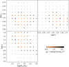 |
Fig. 10. Illustration of the parameter grid explored by our model. Each dot represents one model. The colour code and the symbol size give the reduced |

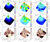 |
Fig. 11. Best-fitting Schwarzschild model of FCC 47. Top row: Voronoi binned kinematic data for FCC 47. Left to right: surface brightness, radial velocity and velocity dispersion. Middle row: best-fit Schwarzschild model. Bottom row: residuals created by subtracting the model from the data. The white patches indicate masked bins. The surface brightness counters are taken from the MGE model (see also Fig. B.1). The plotting ranges are not identical to those shown in Fig. 5. |
The enclosed mass profile including stellar and dark mass is shown in the top panel of Fig. 12. Our model finds a total stellar mass of FCC 47 of M* = 1.5 ± 0.1 × 10¹⁰ M⊙, extrapolated outside of our data coverage. The derived value value is higher than what was found by Saulder et al. (2016), who used photometric integrated magnitudes calibrated with a large sample of spectroscopic SDSS masses, a Kroupa IMF and K-band mass-to-light ratios to estimate the stellar mass to be M* = 6.3 × 10⁹ M⊙. They did not give a value for the uncertainty but they note that the estimate of the photometric stellar mass should be possible within a factor of two. Liu et al. (2019) quoted a stellar mass of M* = 9.3 × 10⁹ M⊙, based on ACSFCS measurements originally used in Turner et al. (2012). These measurements were made using (g − z) colours and the relations from Bell et al. (2003). We find a dark matter fraction of log(Mvir/M*) = 1.5 and a total mass of the dark halo Mvir = 1.1 ± 1.0 × 10¹² M⊙. The uncertainty is large due the lack of data at larger radii. The bottom panel of Fig. 12 shows a radial profile of the shape parameters p and q.
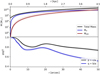 |
Fig. 12. Radial profile of enclosed mass and shape parameters. Top: profile of the enclosed mass for the stellar mass (blue), the dark mass (red) and the total (black). Bottom: radial profile of the geometric shape parameters q and p. The dotted lines indicate the 1σ uncertainty determined from the five best-fitting models. |
Results from the dynamical Schwarzschild model.
7.4. Orbit distribution
The distribution of orbital weights of our model is presented in Figs. 13 and 14. The distribution is shown on the phase space of circularity λi and the intrinsic 3D radius r of a given orbit (see Zhu et al. 2018). We combined the orbit distributions of the five best fitting models. The circularity is used to differentiate between different orbits: |λi| = 1 indicates a circular (cold) orbit, while λi = 0 indicates a radial (hot) orbit. The sign refers to the sense of rotation, and thus negative values indicate counter-rotating orbits. Figure 13 shows the distribution for orbits projected along the short axis z as well as around the long axis x. While z is aligned with the kinematic axis of the rotating disk and main photometric angle of the galaxy, the long axis x is perpendicular. Although due to projection effects, the apparent angle between NSC rotation and the disk is ∼115°, stable orbits only exist around the long or short axis.
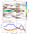 |
Fig. 13. Distribution of orbital weights along short axis. Top: circularity λz of the used orbits versus radius. We show a combination of the five best-fitting models. The dotted lines show the effective radius FCC 47 (Reff, FCC 47 = 30″, Ferguson 1989). Bottom: profile of the mass fractions of rotating (yellow), hot (blue) and counter-rotating orbits (red). The solid lines show the combination of the five best-fitting models (dashed lines). |
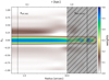 |
Fig. 14. Distribution of orbital weights along long axis of the mean of the five best-fitting models. The dotted lines show the effective radius of the NSC (Reff, NSC = 0.7″, Turner et al. 2012) and FCC 47 (Reff, FCC 47 = 30″, Ferguson 1989). The shaded area shows the region where we lack coverage with the MUSE data along the short axis. |
The orbital distribution around the short axis (Fig. 13) is complex. In the inner region, the orbital structure is dominated by hot and warm orbits (∣λz ∣ < 0.7). Over all radii, the fraction of counter-rotating orbits is high, as also the radial plot of mass fractions of the five best fitting models in the bottom panel of Fig. 13 shows. This explains the negligible rotation in the outskirts of the galaxy as the two counter-rotating populations with warm orbits cancel each others rotation signatures while still showing a high velocity dispersion. This kinematic feature has been routinely observed in galaxies hosting extended counter-rotating stellar components (see Corsini 2014 for a review).
The distribution for the circularity around the long axis shows less structure. It is completely dominated by hot box orbits over all radii. The warm orbits at small radii (λx ∼ 0.25, r ≲ 3″) highlight the rotation of the NSC. The radial extent of these weights are larger than the effective radius of the NSC, but match the apparent size of the NSC in the MUSE data (∼3″). The spots with small weights at r > 10″ are most likely not connected to real features. Instead, they are an effect of the limited size of the orbit library and of the limited coverage of the MUSE data along the short axis that only extends out to ∼10″ along this axis.
The orbital distributions shown in Fig. 13 reveal the nature of the two kinematically decoupled components in FCC 47. The rotation of the disk seen on a ∼2 kpc scale (see Fig. 5) is not a decoupled component as such, instead the high fraction of counter-rotating orbits indicate that this apparent rotating disk is the result of two much more extended counter-rotating populations that show an imbalance on the scale of the disk. Interestingly, according to our model, we see that the counter-rotating population has a larger mass fraction by a few percent on the extend of the disk. The small rotation amplitude of the apparent disk rotation can be explained by this small difference in mass fractions. On the other hand, the NSC appears to be a separate component with a distinct kinematic signature. Besides the NSC, there is no evidence for other populations that show disk-like prolate rotation. The limited spatial resolution of the MUSE data does not allow to estimate a contribution from a central SMBH to this mass.
8. Discussion
FCC 47 is a ETG with M* ∼ 1010 M⊙ in the outskirts of the Fornax cluster with a particularly large NSC and rich GC system. Our MUSE study has revealed several peculiarities that distinguish this galaxy from others, for example the presence of two visible KDCs. In the following we use our comprehensive collection of information to put constraints on the formation history of FCC 47’s massive NSC.
8.1. The star clusters in FCC 47
We first want to discuss our findings for the star clusters in FCC 47. Comparing the NSC with FCC 47’s GC system and the galaxy itself allows us to put constraints on the NSC formation.
8.1.1. The nuclear star cluster
FCC 47 was targeted because of its particularly large NSC with an effective radius of 66 pc (Turner et al. 2012). Using a large sample of NSCs in early- and late-type galaxies, Georgiev et al. (2016) studied various scaling relations between mass and size of the NSC and host mass properties. The observed relation between NSC size and host mass would predict a NSC with an effective radius of ∼20 pc for a galaxy with the stellar mass of FCC 47. However, the observed radius of 66 pc is still within the scatter and there are several other ETGs with NSCs of similar sizes in this mass range. In addition to the size, our data allowed to estimate the stellar mass of the NSC to be ∼7 × 10⁸ M⊙ using stellar population models. This is a massive NSC and is slightly more massive than NSCs of a similar size, but again it lies within the scatter of the NSC size-mass relation (Georgiev et al. 2016). Nonetheless, this high mass places the NSC among the most massive known NSCs (e.g. Sánchez-Janssen et al. 2019).
The NSC constitutes the peak of metallicity and stellar age in FCC 47 and is clearly more metal-rich than the immediate surrounding galaxy, in fact it is possible that a large fraction of the strong central metallicity gradient can be explained by the metal-rich NSC being smeared out by the MUSE PSF. While many NSCs were found to also contain young stellar populations (Rossa et al. 2006; Paudel et al. 2011), the NSC in FCC 47 shows no contribution from young stars (< 10 Gyr). It contains the oldest stellar ages, indicating a quick metal-enrichment and early quenching of star formation. We could identify two subpopulations in the NSC, a dominant population with super-solar metallicities and intermediate [α/Fe], and a secondary component that has a lower metallicity (∼ − 0.4 dex) and a higher alpha-abundance ratio. These two populations could be explained by continuous and efficient self-enrichment of an initially metal-poor and alpha-enhanced stellar population that increased metallicity and decreased [α/Fe] due to the pollution from supernovae Ia ejecta. These supernovae release iron into the interstellar medium within ∼1 Gyr (Thomas et al. 2005), in agreement with the exclusively old ages we found in the NSC. As we could not find different SFHs for the metal-poor and metal-rich subpopulations, the self-enrichment must have stopped early in this picture. Alternatively, the more metal-poor component could indicate NSC mass growth through the accretion of GCs of this chemical composition.
In the study of Lyubenova & Tsatsi (2019) that used high angular resolution IFU SINFONI data of five NSCs of galaxies in the Fornax cluster, the NSC of FCC 47 stood out with having the strongest rotation and consequently having the highest angular momentum of the observed sample. The MUSE data confirmed the rotation of the NSC, but allowed us to set it into context with the rest of the galaxy and we see that the NSC rotates as a KDC around an axis offset by 115° from the main photometric (and rotation) axis of the galaxy. While the NSC in the Milky Way shows evidence for a small misalignment between the rotation of the NSC and the galactic plane (Feldmeier et al. 2014), the gas-rich late-type galaxies studied by Seth et al. (2008b) have NSCs that rotate in the plane of their host. Due to lower intrinsic rotation and a more spherical geometry, kinematically misaligned NSCs could be easier to spot in ETGs.
The NSC in FCC 47 was originally identified as an excess of light at the centre of the galaxy (Turner et al. 2012). Our analysis showed that the NSC is indeed a distinct component of FCC 47, both in its kinematic and stellar population properties.
8.1.2. The globular clusters
The ETG FCC 47 has a rich GC system with more than 300 candidates identified in the ACSFCS (Jordán et al. 2015). We could identify 42 GCs in our MUSE data, with 25 having a spectral S/N high enough to extract their LOS velocity. With this small number GC sample, we could not identify rotating substructures, but we found that the GCs show a large velocity dispersion. This is in agreement with other studies that have established that GCs usually are a dynamical hot system (e.g. Kissler-Patig & Gebhardt 1998; Dabringhausen et al. 2008), supported by velocity dispersion. However, there have been detections of rotating subsystems in other galaxies (e.g. Foster et al. 2016; Forbes et al. 2017). We noted that the blue GC subpopulation shows a larger velocity dispersion than the red GCs, as in most other galaxies (e.g. Schuberth et al. 2010). In addition, the ACSFCS study shows that red GCs are more centrally concentrated and as a consequence the distribution of GC colours shows a radial gradient from red to blue in the outskirts.
From the five GCs that are bright enough to estimate their metallicity, we found four blue GCs that are significantly more metal-poor than the galaxy at their projected distance. The fifth GC is red and has a higher metallicity, similar to the NSC. Combined with the fact that we could not find indications of young ages in the GCs or the stellar light, the bimodality of GC colours in FCC 47 might be truly an effect of a metallicity bimodality, however, we only have five GCs to support this. Using the photometric colours from the ACSFCS and assuming an old age (13 Gyr) for all ACSFCS GC candidates, we estimated that the GC system has a total mass of ∼1 × 10⁸ M⊙. This is only ∼17% the mass found in the NSC.
The larger velocity dispersion, the low metallicities of the blue GCs and the GC colour gradient indicate an ex-situ origin of the blue GC system. Generally, the bimodal colour distribution of GCs as observed in many galaxies is interpreted in this scheme, with the red (metal-rich) GC population having formed in-situ while the blue GCs were accreted through minor mergers with metal-poorer dwarf galaxies (Côté et al. 1998, 2006; Hilker et al. 1999b; Lotz et al. 2004; Peng et al. 2006; Georgiev et al. 2008). The red, metal-rich GC population might have formed together with the NSC and the metal-rich galaxy population, that has a smaller mass fraction and thus is hidden within the metal-poor population of FCC 47, that is particularly dominant at larger radii.
8.2. Constraints on the formation of FCC 47’s nuclear star cluster
Having collected information on the kinematic and stellar population structure of FCC 47 itself, its NSC, and the GCs, we want to explore if we can put constraints on the formation of FCC 47’s massive NSC. We explore the implications of the two most commonly discussed scenarios, accretion of GCs and in-situ formation of the NSC.
8.2.1. Globular cluster accretion scenario
As discussed in the introduction, in the GC accretion scenario, the NSC forms from the (dry) accretion of in-spiralling GCs that make their way to the centre due to dynamical friction. Although the in-fall of GCs with random orbits can result in a low net angular momentum of the NSC, simulations have shown that some NSCs can have significant rotation. In the case of the NSC of FCC 47, a comparison to N-body simulations (Antonini et al. 2012; Perets & Mastrobuono-Battisti 2014; Tsatsi et al. 2017) has shown that this high angular momentum can still be explained by gas-free accretion of GCs, but requires a preferred in-fall orbital direction as discussed by Lyubenova & Tsatsi (2019). However, we could not find any indication for rotation substructure in the GC population, possible due to the low numbers of available GC LOS velocities and an incomplete spatial coverage. In a future wide-field study of the kinematics of the red GC subpopulation that might share the high metallicity of the NSC could give a handle on the contribution of GC accretion to the NSC mass build up. However, the subsequent evolution of the cluster system and merger events of the host galaxy could have removed any rotation substructure within the GCs.
The old ages and the absence of young populations in the NSC are consistent with the accretion of gas-free GCs. We find that the NSC constitutes the metal-rich peak of FCC 47 and is significantly more metal-rich than the blue (metal-poor) GC population, however, we find at least one red GC that has a similar metallicity. Our current sample of GCs with metallicity measurements is very limited, but the comparison of GC colours shows that there probably still are GCs in FCC 47 with metallicities similar to the NSC. These red GCs are also more centrally concentrated and thus it is possible that the NSC has formed or grown by accreting such GCs, similar to the GCs found in the bulge of the MW (e.g. Côté 1999; Muñoz et al. 2017, 2018). The presence of a minor more metal-poor population in the NSC, might indicate some accretion of old, metal-poor and alpha-enhanced stars, possibly also accreted in an in-spiral of a few metal-poor GCs. However, it is unclear if the steep central metallicity gradient can be explained by GC in-spiral because the disk region already shows significantly lower metallicites or whether (and how much) additional gas accretion would be needed.
Similarly, the composite formation scenario proposed by Guillard et al. (2016) could give a viable explanation for the formation of the NSC in FCC 47. In their scenario, a massive gas-rich GC forms close to the centre and spirals inwards within a few Gyr, possibly followed by a merger with a second gas-rich GC. Depending on whether a second GC falls to the centre, this model predicts significant rotation in the formed NSC and a fast quenching of star formation in the centre because of gas being expelled, in agreement with the old age and high metallicity we find for the NSC in FCC 47. However, it is unclear if this scenario can explain the KDC with the offset rotation axis and the described accretion of only two massive GCs is not viable for FCC 47. To explain its mass, a large number of star clusters must have merged within the first Gyr of the galaxy.
Independent of the kinematic and chemical structure of the NSC and the GCs, the high mass of the NSC makes formation solely by GC-accretion unlikely. As our estimate shows, the NSC is much more massive than the total GC system as observed today. To explain its mass of ∼7 × 10⁸ M⊙, it must have accreted early-on hundreds of GCs that must have been quite massive (> 106 M⊙) to explain the high (and homogeneous) metallicity. Modelling the effects of dynamical friction, evolution including mass loss and tidal stripping on the GC system of the MW and M 87, Gnedin et al. (2014) found that GC accretion can contribute a large fraction of mass to NSCs in galaxies with M* < 1011 M⊙. However, following their predicted scaling between NSC and galaxy stellar mass, FCC 47’s NSC should have a mass of ∼1 × 10⁸ M⊙ assuming growth through GC accretion. This estimate would increase if FCC 47 had been extremely efficient in forming massive metal-rich star clusters early on, but it is questionable how such a large population of metal-rich GCs could have formed.
We therefore conclude that the formation of the NSC in FCC47 is unlikely to have been dominated by the gas-free accretion of old GCs. However, from simple dynamical arguments, it follows that there must have been some GC accretion in such a rich GC system and the accretion of young metal-rich star clusters early-on is still possible. Detailed modelling that accounts for the properties of FCC 47’s GC system would be needed to get a handle on the relative fraction of mass build up via dry GC accretion.
8.2.2. In-situ formation
The formation of the NSC through in-situ formation from infalling gas can explain the high mass and high metallicity better, but requires that a large supply of gas has been funnelled originally into the centre of FCC 47. This supply must have been quickly exhausted after a short period of efficient star formation and self-enrichment. With our data, we cannot constrain the mechanisms that have stopped the star formation in the NSC and the rest of the galaxy. We do not know if the gas was simply exhausted or it was removed, possibly due to interactions in the Fornax cluster environment, stellar feedback, or feedback from an active galactic nucleus.
As the study of Lyubenova & Tsatsi (2019) has shown, the high angular momentum of the NSC is inconsistent with formation via the in-spiral of GCs from random directions, so would need coherent anisotropic accretion of GCs. Therefore, the in-situ formation from infalling gas might be a more viable explanation for the formation of the NSC in FCC 47. In this scenario, the infalling gas would inherit the angular momentum from its origin. However, there is no indication of other stellar populations rotating around the same axis as the NSC, neither in the galaxy main body nor within the GC population, but a larger sample of (red) GC velocities is needed to confirm this. Instead, the rotation axis of the NSC is offset with respect to the photometric axis and main rotation axis of the galaxy. The origin of the kinematically decoupled rotation of the NSC might not be connected to intrinsic formation scenarios as discussed, but could be evidence for a major merger that has altered FCC 47 kinematic structure significantly. Such a merger and the corresponding merger of the NSCs of the progenitor galaxies could also explain the high mass of FCC 47’s NSC.
8.2.3. Evidence for merger history of FCC 47
KDCs are not a rare phenomenon, especially in massive ETGs (M* > 1010.8 M⊙, Krajnović et al. 2013). Classical KDCs have kpc-sizes, similar to the rotating disk structure in FCC 47. Our dynamical model shows that the disk KDC is not truly decoupled, similar to the KDC in NGC 4365 (van den Bosch et al. 2008; Nedelchev et al. 2019). Conversely, the NSC is a distinct kinematic component and is in its size comparable to the class of compact KDCs with sizes of ∼100 pc (McDermid et al. 2007). In contrast to the NSC of FCC 47, these more compact KDCs usually have noticeably younger ages (McDermid et al. 2006), although the apparent size of the NSC in the MUSE data (∼3″ ≈ 250 pc) places it in between these two classifications.
Simulations of galaxy mergers have been able to explain the formation of KDCs, but they always require a major merger between massive galaxies. The central kinematic decoupling arises if, for example, gas dissipation, retrograde merger orbits or the merger of gas-rich disks are incorporated in the simulations (Balcells & Quinn 1990; Barnes & Hernquist 1992; Jesseit et al. 2007; Bois et al. 2011). Tsatsi et al. (2015) showed that kpc-sized KDCs can also form in a prograde merger of two disk galaxies during which reactive forces create short-lived reversal of the orbital spin.
Rantala et al. (2019) shows that KDCs may also arise from orbit reversals of the central SMBH caused by gravitational torques from expelled material in the dissipationless merger of two massive ETGs. For binary mergers of massive ETGs (each M* > 8 × 10¹⁰ M⊙) with very massive SMBHs (each > 109 M⊙), they even find multiple KDCs, similar to what we found in FCC 47, however, the simulated KDCs still share a single rotation axis aligned with the minor axis of the galaxy. In case the described scenario scales down to lower-mass galaxies such as FCC 47, the simulations predict a very massive SMBH as well as a tangential velocity anisotropy in the centre. Both the presence of a SMBH and a central tangentially biased velocity structure could not be tested with the MUSE data due to the limited spatial resolution but could be measured by improving the current dynamical orbit-based model by including high angular resolution data of the central region, for example by incorporating the SINFONI data into the existing model in a future study.
Although current simulations might not be sufficient to explain the KDCs in FCC 47, the presence of the two apparent KDCs and the two counter-rotating populations seems to be strong evidence of at least one major merger. In particular, the presence of two decoupled components in combination with the exclusively old ages is intriguing. The kinematics could suggest a scenario where the NSC with its decoupled rotation has fallen into the already formed galaxy, perhaps as the remnant nucleus of a destroyed galaxy. However, following the mass-metallicity relation (e.g. Gallazzi et al. 2005; Kirby et al. 2013), the high metallicity of the NSC would then imply that it must have formed in an originally massive galaxy, similar to FCC 47. Alternatively, the NSC might have formed as a red nugget at high redshift and would have ended up as a metal-rich compact elliptical (cE) or massive relic (Ferré-Mateu et al. 2017; Martín-Navarro et al. 2019), but instead got captured by FCC 47. This scenario could explain the metallicity as many cEs are known to have a relatively high metallicity for their mass (Zhang et al. 2018).
In comparison to other galaxies of the Virgo and Fornax cluster, FCC 47 not only has a large and massive NSC (Turner et al. 2012), but also has a higher specific frequency of GCs within one effective radius than other galaxies of similar mass (Liu et al. 2019). This might imply that the formation of the NSC and the red, centrally concentrated GC system is connected. Thus, a scenario in which the NSC is an original part of the galaxy might be favoured. In such a scenario, the NSC, the metal-rich part of galaxy, and the red, metal-rich GCs could have formed together in clumpy, bursty star formation at high redshift (see also Beasley et al. 2018). The galaxy then later underwent at least one major merger that created the counter-rotating populations and younger, more metal-poor outskirts. Specialised simulations would be required to test whether the decoupled rotation of the NSC could have survived the subsequent evolution of the galaxy or whether the kinematic decoupling itself could be a result of second major merger.
Independent of the exact formation scenario that has caused the peculiar kinematic structure of FCC 47, the presence of KDCs indicate the importance of mergers in the formation of both galaxy and NSC. Thus, studying other massive NSCs and their hosts is required to determine if the commonly discussed NSC formation scenarios are sufficient to explain the formation of the most massive NSCs in general.
9. Conclusions
In this paper, we presented a comprehensive study of the kinematic and stellar population structure of the early-type galaxy FCC47 using MUSE WFM AO SV data. We have analysed both the integrated stellar light and GCs as discrete tracers of the kinematic and chemical structure, connecting the results to the kinematic and chemical study of the NSC. Its particularly large size allowed us to resolve its structure. We summarise our results as follows:
– We found that FCC 47 shows a complex velocity structure with two KDCs on different scales. While there is no significant rotation on large scales, a rotating disk structure with a rotation amplitude of ∼20 km s−1 is found with an extent of ∼2 kpc. In addition, our MUSE observation confirms the high angular momentum, strong rotation and high velocity dispersion of the NSC as discovered in earlier work. The rotation axis of the NSC and of the inner disk are offset by ∼115°, constituting a second KDC.
– We constructed a Schwarzschild model to reveal FCC 47’s orbital structure. According to this model, the main body of FCC 47 consists of two counter-rotating populations. On large scales, the counter-rotation cancels out any rotation signature. Near the centre, the two counter-rotating populations show an imbalance, thus creating the emergence of a inner rotating disk structure. The NSC appears to be truely kinematically decoupled and we find no indication of other populations showing the same sense of rotation. The Schwarzschild model determined the total stellar mass of FCC 47 to be M* = 1.6 × 10¹⁰ M⊙.
– FCC 47 is overall old (> 8 Gyr) and shows an age gradient from very old ages in the centre to younger ages in the outskirts. We did not find any evidence of young populations, gas or dust. While the galaxy is metal-poorer on larger scales, we find that the centre reaches solar metallicities and shows a strong central gradient that flattens outwards. The region of high metallicity matches the extent of the NSC rotation structure. We therefore assumed that the high metallicity is associated to the NSC while the rest of the galaxy is significantly more metal-poor with a shallow metallicity gradient. The NSC does not stand out in the map of light element abundance ratios ([α/Fe]).
– Dividing FCC 47 into the NSC, the (rotating) disk and the main galaxy body showed that the NSC is dominated (∼70% in mass) by a metal-rich, old stellar population. This mass fraction decreases down to 47% in the disk and to < 30% in the outskirts, where the galaxy is dominated by a more metal-poor population.
– Studying the galaxy-subtracted NSC spectrum confirmed the old age of the NSC, but we found two chemically distinct subpopulations: a dominating (67%) metal-rich population with intermediate light element abundance ratio and a secondary population with lower metallicity and higher [α/Fe]. From the stellar population analysis, we found that the NSC is very massive (M ∼ 7 × 10⁸ M⊙).
– We extracted MUSE spectra of 42 GCs using an ancillary catalogue from Jordán et al. (2015) as reference. 25 of these have a sufficient spectral S/N to determine their LOS velocity and a sub-sample of five GCs is bright enough for an estimate of their metallicities.
– Within our sample of GC velocities, we did not see any rotation, but the blue GC population shows a larger velocity dispersion than the red population. Four of the five GCs that allowed a measurement of their metallicity have blue colours and are found to be significantly metal-poorer than the galaxy, while the fifth GC is associated with the red GC population and has a higher metallicity similar to the NSC. The red GCs could have formed together with the NSC and the metal-rich stellar population. Based on photometric metallicities, we estimated the total mass in GCs to be ∼1 × 10⁸ M⊙.
– We interpreted our results with respect to the most discussed formation channels of NSCs: the gas-free GC accretion and the in-situ formation scenario. With its high angular momentum, high mass and high metallicity, the NSC of FCC47 is unlikely to have formed dominantly by accreting non-rotating, metal-poor GCs as we find them in FCC 47 today. However, we could not rule out that the NSC has formed a fraction of its mass by accreting more metal-rich GCs or gas-rich massive star clusters early on. Possibly, the decoupled kinematics of the NSC are not an effect of the formation pathway, but rather are the result of a major merger that has altered FCC 47’s kinematic structure.
To constrain the relative contribution of the GC-accretion and in-situ formation channel, a comparison with specialised models is required. To accurately constrain the GC-accretion channel, a more in-depth view on the kinematics with more LOS velocities and a larger spatial coverage of the red GC population is required because these seem to share the high metallicity of the NSC.
FCC 47 was targeted as MUSE WFM + AO SV target because of its large, strongly-rotating NSC and the rich GC system. Being a ETG in the outskirts of the Fornax cluster, the wealth of complexity in this galaxy has been surprising: we found two KDCs, a sharp central metallicity peak, and FCC 47-UCD1. As we argue in Fahrion et al. (2019), the UCD could be the stripped nucleus of a disrupted dwarf galaxy and would therefore indicate a minor merger in FCC 47’s past. In addition, the KDCs most likely are evidence of at least one major merger event that has altered the kinematic structure of the galaxy significantly.
SN, z = NGC × 100.4(Mz + 15) with the total z-band magnitude Mz and the number of GCs NGC.
FDS is a large scale survey of the Fornax galaxy cluster with the VLT Survey Telescope (VST) that covers ∼26 square degrees around the central galaxy NGC 1399 in u, g, r and i-bands.
Acknowledgments
We thank the anonymous referee for helpful comments and suggestions that improved this manuscript. This work is based on observations collected at the European Organization for Astronomical Research in the Southern Hemisphere under the ESO programme 60.A-9192. GvdV acknowledges funding from the European Research Council (ERC) under the European Union’s Horizon 2020 research and innovation programme under grant agreement No 724857 (Consolidator Grant ArcheoDyn). J. F-B acknowledges support from grant AYA2016-77237-C3-1-P from the Spanish Ministry of Economy and Competitiveness (MINECO). E.M.C. acknowledges financial support from Padua University through grants DOR1715817/17, DOR1885254/18, and BIRD164402/16. RMcD is the recipient of an Australian Research Council Future Fellowship (project number FT150100333). LZ acknowledges support from Shanghai Astronomical Observatory, Chinese Academy of Sciences under grant NO.Y895201009
References
- Agarwal, M., & Milosavljević, M. 2011, ApJ, 729, 35 [NASA ADS] [CrossRef] [Google Scholar]
- Antonini, F. 2013, ApJ, 763, 62 [NASA ADS] [CrossRef] [Google Scholar]
- Antonini, F. 2014, ApJ, 794, 106 [NASA ADS] [CrossRef] [Google Scholar]
- Antonini, F., Capuzzo-Dolcetta, R., Mastrobuono- Battisti, A., & Merritt, D. 2012, ApJ, 750, 111 [NASA ADS] [CrossRef] [Google Scholar]
- Antonini, F., Barausse, E., & Silk, J. 2015, ApJ, 812, 72 [NASA ADS] [CrossRef] [Google Scholar]
- Arca-Sedda, M., & Capuzzo-Dolcetta, R. 2014, ApJ, 785, 51 [NASA ADS] [CrossRef] [Google Scholar]
- Bacon, R., Copin, Y., Monnet, G., et al. 2001, MNRAS, 326, 23 [NASA ADS] [CrossRef] [Google Scholar]
- Balcells, M., & Quinn, P. J. 1990, ApJ, 361, 381 [NASA ADS] [CrossRef] [Google Scholar]
- Barnes, J. E., & Hernquist, L. 1992, Annu. Rev. Astron. Astrophys., 30, 705 [Google Scholar]
- Beasley, M. A., Trujillo, I., Leaman, R., & Montes, M. 2018, Nature, 555, 483 [NASA ADS] [CrossRef] [Google Scholar]
- Bekki, K. 2007, PASA, 24, 77 [NASA ADS] [CrossRef] [Google Scholar]
- Bekki, K., Couch, W. J., & Shioya, Y. 2006, ApJ, 642, L133 [NASA ADS] [CrossRef] [Google Scholar]
- Bell, E. F., McIntosh, D. H., Katz, N., & Weinberg, M. D. 2003, ApJS, 149, 289 [NASA ADS] [CrossRef] [Google Scholar]
- Bendinelli, O. 1991, ApJ, 366, 599 [NASA ADS] [CrossRef] [Google Scholar]
- Blakeslee, J. P., Jordán, A., Mei, S., et al. 2009, ApJ, 694, 556 [NASA ADS] [CrossRef] [Google Scholar]
- Boecker, A., Leaman, R., van de Ven, G., et al. 2019, MNRAS, submitted [arXiv:1903.11089] [Google Scholar]
- Bois, M., Emsellem, E., Bournaud, F., et al. 2011, MNRAS, 416, 1654 [NASA ADS] [CrossRef] [Google Scholar]
- Böker, T., Laine, S., van der Marel, R. P., et al. 2002, AJ, 123, 1389 [NASA ADS] [CrossRef] [Google Scholar]
- Böker, T., Sarzi, M., McLaughlin, D. E., et al. 2004, AJ, 127, 105 [NASA ADS] [CrossRef] [Google Scholar]
- Burkert, A., & Forbes, D. 2019, MNRAS, submitted [arXiv:1901.00900] [Google Scholar]
- Cappellari, M. 2002, MNRAS, 333, 400 [NASA ADS] [CrossRef] [Google Scholar]
- Cappellari, M. 2017, MNRAS, 466, 798 [NASA ADS] [CrossRef] [Google Scholar]
- Cappellari, M., & Copin, Y. 2003, MNRAS, 342, 345 [NASA ADS] [CrossRef] [Google Scholar]
- Cappellari, M., & Emsellem, E. 2004, PASP, 116, 138 [NASA ADS] [CrossRef] [Google Scholar]
- Cappellari, M., Emsellem, E., Krajnović, D., et al. 2011, MNRAS, 413, 813 [NASA ADS] [CrossRef] [Google Scholar]
- Capuzzo-Dolcetta, R. 1993, ApJ, 415, 616 [NASA ADS] [CrossRef] [Google Scholar]
- Capuzzo-Dolcetta, R., & Miocchi, P. 2008, ApJ, 681, 1136 [NASA ADS] [CrossRef] [Google Scholar]
- Corsini, E. M. 2014, in Multi-spin Galaxies, eds. E. Iodice, & E. M. Corsini, ASP Conf. Ser., 486, 51 [NASA ADS] [Google Scholar]
- Côté, P. 1999, AJ, 118, 406 [NASA ADS] [CrossRef] [Google Scholar]
- Côté, P., Marzke, R. O., & West, M. J. 1998, ApJ, 501, 554 [NASA ADS] [CrossRef] [Google Scholar]
- Côté, P., Piatek, S., Ferrarese, L., et al. 2006, ApJS, 165, 57 [NASA ADS] [CrossRef] [MathSciNet] [Google Scholar]
- Dabringhausen, J., Hilker, M., & Kroupa, P. 2008, MNRAS, 386, 864 [NASA ADS] [CrossRef] [Google Scholar]
- den Brok, M., Peletier, R. F., Seth, A., et al. 2014, MNRAS, 445, 2385 [NASA ADS] [CrossRef] [Google Scholar]
- Dopita, M., Rhee, J., Farage, C., et al. 2010, Ap&SS, 327, 245 [NASA ADS] [CrossRef] [Google Scholar]
- Drinkwater, M. J., Jones, J. B., Gregg, M. D., & Phillipps, S. 2000, PASA, 17, 227 [NASA ADS] [CrossRef] [Google Scholar]
- Efstathiou, G., Ellis, R. S., & Carter, D. 1982, MNRAS, 201, 975 [NASA ADS] [Google Scholar]
- Eigenthaler, P., Puzia, T. H., Taylor, M. A., et al. 2018, ApJ, 855, 142 [NASA ADS] [CrossRef] [Google Scholar]
- Emsellem, E., Monnet, G., & Bacon, R. 1994, A&A, 285, 723 [NASA ADS] [Google Scholar]
- Emsellem, E., Cappellari, M., Krajnović, D., et al. 2007, MNRAS, 379, 401 [NASA ADS] [CrossRef] [Google Scholar]
- Emsellem, E., van der Burg, R. F. J., Fensch, J., et al. 2019, A&A, 625, A76 [NASA ADS] [CrossRef] [EDP Sciences] [Google Scholar]
- Erwin, P. 2015, ApJ, 799, 226 [NASA ADS] [CrossRef] [Google Scholar]
- Fahrion, K., Georgiev, I., Hilker, M., et al. 2019, A&A, 625, A50 [NASA ADS] [CrossRef] [EDP Sciences] [Google Scholar]
- Falcón-Barroso, J., Sánchez-Blázquez, P., Vazdekis, A., et al. 2011, A&A, 532, A95 [NASA ADS] [CrossRef] [EDP Sciences] [Google Scholar]
- Feldmeier, A., Neumayer, N., Seth, A., et al. 2014, A&A, 570, A2 [NASA ADS] [CrossRef] [EDP Sciences] [Google Scholar]
- Ferguson, H. C. 1989, AJ, 98, 367 [Google Scholar]
- Ferrarese, L., & Merritt, D. 2000, ApJ, 539, L9 [NASA ADS] [CrossRef] [Google Scholar]
- Ferrarese, L., Côté, P., Dalla Bontà, E., et al. 2006, ApJ, 644, L21 [NASA ADS] [CrossRef] [Google Scholar]
- Ferré-Mateu, A., Trujillo, I., Martín-Navarro, I., et al. 2017, MNRAS, 467, stx171 [CrossRef] [Google Scholar]
- Forbes, D. A., Alabi, A., Brodie, J. P., et al. 2017, AJ, 153, 114 [NASA ADS] [CrossRef] [Google Scholar]
- Forbes, D. A., Read, J. I., Gieles, M., & Collins, M. L. M. 2018, MNRAS, 481, 5592 [NASA ADS] [CrossRef] [Google Scholar]
- Foster, C., Pastorello, N., Roediger, J., et al. 2016, MNRAS, 457, 147 [NASA ADS] [CrossRef] [Google Scholar]
- Franx, M., & Illingworth, G. D. 1988, ApJ, 327, L55 [NASA ADS] [CrossRef] [Google Scholar]
- Freudling, W., Romaniello, M., Bramich, D. M., et al. 2013, A&A, 559, A96 [NASA ADS] [CrossRef] [EDP Sciences] [Google Scholar]
- Gallazzi, A., Charlot, S., Brinchmann, J., White, S. D. M., & Tremonti, C. A. 2005, MNRAS, 362, 41 [NASA ADS] [CrossRef] [Google Scholar]
- Gebhardt, K., Bender, R., Bower, G., et al. 2000, ApJ, 539, L13 [NASA ADS] [CrossRef] [Google Scholar]
- Georgiev, I. Y., & Böker, T. 2014, MNRAS, 441, 3570 [NASA ADS] [CrossRef] [Google Scholar]
- Georgiev, I. Y., Goudfrooij, P., Puzia, T. H., & Hilker, M. 2008, AJ, 135, 1858 [NASA ADS] [CrossRef] [Google Scholar]
- Georgiev, I. Y., Hilker, M., Puzia, T. H., Goudfrooij, P., & Baumgardt, H. 2009, MNRAS, 396, 1075 [NASA ADS] [CrossRef] [Google Scholar]
- Georgiev, I. Y., Puzia, T. H., Goudfrooij, P., & Hilker, M. 2010, MNRAS, 406, 1967 [NASA ADS] [Google Scholar]
- Georgiev, I. Y., Böker, T., Leigh, N., Lützgendorf, N., & Neumayer, N. 2016, MNRAS, 457, 2122 [Google Scholar]
- Glass, L., Ferrarese, L., Côté, P., et al. 2011, ApJ, 726, 31 [NASA ADS] [CrossRef] [Google Scholar]
- Gnedin, O. Y., Ostriker, J. P., & Tremaine, S. 2014, ApJ, 785, 71 [NASA ADS] [CrossRef] [Google Scholar]
- Graham, A. W., & Driver, S. P. 2007, ApJ, 655, 77 [NASA ADS] [CrossRef] [Google Scholar]
- Graham, A. W., & Spitler, L. R. 2009, MNRAS, 397, 2148 [NASA ADS] [CrossRef] [Google Scholar]
- Guérou, A., Emsellem, E., Krajnović, D., et al. 2016, A&A, 591, A143 [NASA ADS] [CrossRef] [EDP Sciences] [Google Scholar]
- Guillard, N., Emsellem, E., & Renaud, F. 2016, MNRAS, 461, 3620 [NASA ADS] [CrossRef] [Google Scholar]
- Harris, W. E., Harris, G. L. H., & Alessi, M. 2013, ApJ, 772, 82 [NASA ADS] [CrossRef] [Google Scholar]
- Hartmann, M., Debattista, V. P., Seth, A., Cappellari, M., & Quinn, T. R. 2011, MNRAS, 418, 2697 [NASA ADS] [CrossRef] [Google Scholar]
- Hilker, M., Infante, L., Vieira, G., Kissler-Patig, M., & Richtler, T. 1999a, A&AS, 134, 75 [NASA ADS] [CrossRef] [EDP Sciences] [Google Scholar]
- Hilker, M., Infante, L., & Richtler, T. 1999b, ApJS, 138, 55 [Google Scholar]
- Hopkins, P. F., Murray, N., & Thompson, T. A. 2009, MNRAS, 398, 303 [NASA ADS] [CrossRef] [Google Scholar]
- Iodice, E., Capaccioli, M., Grado, A., et al. 2016, ApJ, 820, 42 [NASA ADS] [CrossRef] [Google Scholar]
- Jesseit, R., Naab, T., Peletier, R. F., & Burkert, A. 2007, MNRAS, 376, 997 [NASA ADS] [CrossRef] [Google Scholar]
- Jordán, A., Blakeslee, J. P., Côté, P., et al. 2007, ApJS, 169, 213 [NASA ADS] [CrossRef] [Google Scholar]
- Jordán, A., Peng, E. W., Blakeslee, J. P., et al. 2015, ApJS, 221, 13 [NASA ADS] [CrossRef] [Google Scholar]
- Kacharov, N., Neumayer, N., Seth, A. C., et al. 2018, MNRAS, 480, 1973 [NASA ADS] [CrossRef] [Google Scholar]
- Kirby, E. N., Cohen, J. G., Guhathakurta, P., et al. 2013, ApJ, 779, 102 [NASA ADS] [CrossRef] [Google Scholar]
- Kissler-Patig, M., & Gebhardt, K. 1998, AJ, 116, 2237 [NASA ADS] [CrossRef] [Google Scholar]
- Kormendy, J., & Ho, L. C. 2013, Annu. Rev. Astron. Astrophys., 51, 511 [Google Scholar]
- Krajnović, D., Karick, A. M., Davies, R. L., et al. 2013, MNRAS, 433, 2812 [NASA ADS] [CrossRef] [Google Scholar]
- Krajnović, D., Weilbacher, P. M., Urrutia, T., et al. 2015, MNRAS, 452, 2 [NASA ADS] [CrossRef] [Google Scholar]
- Liu, Y., Peng, E. W., Jordán, A., et al. 2019, ApJ, 875, 156 [NASA ADS] [CrossRef] [Google Scholar]
- Lotz, J. M., Miller, B. W., & Ferguson, H. C. 2004, ApJ, 613, 262 [NASA ADS] [CrossRef] [MathSciNet] [Google Scholar]
- Lyubenova, M., & Tsatsi, A. 2019, A&A, in press, https://doi.org/10.1051/0004-6361/201833954 [Google Scholar]
- Lyubenova, M., van den Bosch, R. C. E., Côté, P., et al. 2013, MNRAS, 431, 3364 [NASA ADS] [CrossRef] [Google Scholar]
- Magorrian, J., Tremaine, S., Richstone, D., et al. 1998, AJ, 115, 2285 [NASA ADS] [CrossRef] [Google Scholar]
- Martín-Navarro, I., van de Ven, G., & Yıldırım, A. 2019, MNRAS, 487, 1468 [Google Scholar]
- McDermid, R. M., Emsellem, E., Shapiro, K. L., et al. 2006, MNRAS, 373, 906 [Google Scholar]
- McDermid, R. M., Emsellem, E., Shapiro, K. L., et al. 2007, in Stellar Populations as Building Blocks of Galaxies, eds. A. Vazdekis, & R. Peletier, IAU Symp., 241, 399 [NASA ADS] [Google Scholar]
- McDermid, R. M., Alatalo, K., Blitz, L., et al. 2015, MNRAS, 448, 3484 [NASA ADS] [CrossRef] [Google Scholar]
- Mihos, J. C., & Hernquist, L. 1994, ApJ, 437, L47 [NASA ADS] [CrossRef] [Google Scholar]
- Milosavljević, M. 2004, ApJ, 605, L13 [NASA ADS] [CrossRef] [Google Scholar]
- Monnet, G., Bacon, R., & Emsellem, E. 1992, A&A, 253, 366 [NASA ADS] [Google Scholar]
- Muñoz, C., Villanova, S., Geisler, D., et al. 2017, A&A, 605, A12 [NASA ADS] [CrossRef] [EDP Sciences] [Google Scholar]
- Muñoz, C., Geisler, D., Villanova, S., et al. 2018, A&A, 620, A96 [NASA ADS] [CrossRef] [EDP Sciences] [Google Scholar]
- Navarro, J. F., Frenk, C. S., & White, S. D. M. 1996, ApJ, 462, 563 [NASA ADS] [CrossRef] [Google Scholar]
- Nedelchev, B., Coccato, L., Corsini, E. M., et al. 2019, A&A, 623, A87 [NASA ADS] [CrossRef] [EDP Sciences] [Google Scholar]
- Neumayer, N., & Walcher, C. J. 2012, Adv. Astron., 2012, 709038 [NASA ADS] [Google Scholar]
- Neumayer, N., Walcher, C. J., Andersen, D., et al. 2011, MNRAS, 413, 1875 [NASA ADS] [CrossRef] [Google Scholar]
- Norris, M. A., Escudero, C. G., Faifer, F. R., et al. 2015, MNRAS, 451, 3615 [NASA ADS] [CrossRef] [Google Scholar]
- Ordenes-Briceño, Y., Puzia, T. H., Eigenthaler, P., et al. 2018, ApJ, 860, 4 [NASA ADS] [CrossRef] [Google Scholar]
- Paudel, S., Lisker, T., & Kuntschner, H. 2011, MNRAS, 413, 1764 [NASA ADS] [CrossRef] [Google Scholar]
- Peng, E. W., Jordán, A., Côté, P., et al. 2006, ApJ, 639, 95 [NASA ADS] [CrossRef] [Google Scholar]
- Perets, H. B., & Mastrobuono-Battisti, A. 2014, ApJ, 784, L44 [NASA ADS] [CrossRef] [Google Scholar]
- Pfeffer, J., & Baumgardt, H. 2013, MNRAS, 433, 1997 [NASA ADS] [CrossRef] [Google Scholar]
- Phillipps, S., Drinkwater, M. J., Gregg, M. D., & Jones, J. B. 2001, ApJ, 560, 201 [NASA ADS] [CrossRef] [Google Scholar]
- Pietrinferni, A., Cassisi, S., Salaris, M., & Castelli, F. 2004, ApJ, 612, 168 [NASA ADS] [CrossRef] [Google Scholar]
- Pietrinferni, A., Cassisi, S., Salaris, M., & Castelli, F. 2006, ApJ, 642, 797 [NASA ADS] [CrossRef] [Google Scholar]
- Pinna, F., Falcón-Barroso, J., Martig, M., et al. 2019, A&A, 623, A19 [NASA ADS] [CrossRef] [EDP Sciences] [Google Scholar]
- Pizzella, A., Corsini, E. M., Morelli, L., et al. 2002, ApJ, 573, 131 [NASA ADS] [CrossRef] [Google Scholar]
- Portaluri, E., Corsini, E. M., Morelli, L., et al. 2013, MNRAS, 433, 434 [NASA ADS] [CrossRef] [Google Scholar]
- Puzia, T. H., Paolillo, M., Goudfrooij, P., et al. 2014, ApJ, 786, 78 [NASA ADS] [CrossRef] [Google Scholar]
- Rantala, A., Johansson, P. H., Naab, T., Thomas, J., & Frigo, M. 2019, ApJ, 872, L17 [NASA ADS] [CrossRef] [Google Scholar]
- Rossa, J., van der Marel, R. P., Böker, T., et al. 2006, AJ, 132, 1074 [NASA ADS] [CrossRef] [Google Scholar]
- Sánchez-Blázquez, P., Rosales-Ortega, F. F., Méndez-Abreu, J., et al. 2014, A&A, 570, A6 [NASA ADS] [CrossRef] [EDP Sciences] [Google Scholar]
- Sánchez-Janssen, R., Côté, P., Ferrarese, L., et al. 2019, ApJ, 878, 18 [NASA ADS] [CrossRef] [Google Scholar]
- Sarzi, M., Iodice, E., Coccato, L., et al. 2018, A&A, 616, A121 [NASA ADS] [CrossRef] [EDP Sciences] [Google Scholar]
- Saulder, C., van Kampen, E., Chilingarian, I. V., Mieske, S., & Zeilinger, W. W. 2016, A&A, 596, A14 [NASA ADS] [CrossRef] [EDP Sciences] [Google Scholar]
- Schinnerer, E., Böker, T., Meier, D. S., & Calzetti, D. 2008, ApJ, 684, L21 [NASA ADS] [CrossRef] [Google Scholar]
- Schödel, R., Merritt, D., & Eckart, A. 2009, A&A, 502, 91 [NASA ADS] [CrossRef] [EDP Sciences] [Google Scholar]
- Schuberth, Y., Richtler, T., Hilker, M., et al. 2010, A&A, 513, A52 [NASA ADS] [CrossRef] [EDP Sciences] [Google Scholar]
- Scorza, C., & Bender, R. 1995, A&A, 293, 20 [NASA ADS] [Google Scholar]
- Scott, N., Davies, R. L., Houghton, R. C. W., et al. 2014, MNRAS, 441, 274 [NASA ADS] [CrossRef] [Google Scholar]
- Seth, A. C., Dalcanton, J. J., Hodge, P. W., & Debattista, V. P. 2006, ApJ, 132, 2539 [Google Scholar]
- Seth, A., Agüeros, M., Lee, D., & Basu-Zych, A. 2008a, ApJ, 678, 116 [NASA ADS] [CrossRef] [Google Scholar]
- Seth, A. C., Blum, R. D., Bastian, N., Caldwell, N., & Debattista, V. P. 2008b, ApJ, 687, 997 [NASA ADS] [CrossRef] [Google Scholar]
- Seth, A. C., Cappellari, M., Neumayer, N., et al. 2010, ApJ, 714, 713 [NASA ADS] [CrossRef] [Google Scholar]
- Soto, K. T., Lilly, S. J., Bacon, R., Richard, J., & Conseil, S. 2016, MNRAS, 458, 3210 [NASA ADS] [CrossRef] [Google Scholar]
- Spengler, C., Côté, P., Roediger, J., et al. 2017, ApJ, 849, 55 [NASA ADS] [CrossRef] [Google Scholar]
- Spitler, L. R., & Forbes, D. A. 2009, MNRAS, 392, L1 [NASA ADS] [CrossRef] [Google Scholar]
- Stetson, P. B. 1987, PASP, 99, 191 [NASA ADS] [CrossRef] [Google Scholar]
- Strader, J., Seth, A. C., Forbes, D. A., et al. 2013, ApJ, 775, L6 [NASA ADS] [CrossRef] [Google Scholar]
- Thomas, D., Maraston, C., Bender, R., & Mendes de Oliveira, C. 2005, ApJ, 621, 673 [NASA ADS] [CrossRef] [Google Scholar]
- Tremaine, S. D., Ostriker, J. P., & Spitzer, Jr., L. 1975, ApJ, 196, 407 [NASA ADS] [CrossRef] [Google Scholar]
- Tsatsi, A., Macciò, A. V., van de Ven, G., & Moster, B. P. 2015, ApJ, 802, L3 [NASA ADS] [CrossRef] [Google Scholar]
- Tsatsi, A., Mastrobuono-Battisti, A., van de Ven, G., et al. 2017, MNRAS, 464, 3720 [NASA ADS] [CrossRef] [Google Scholar]
- Turner, M. L., Côté, P., Ferrarese, L., et al. 2012, ApJS, 203, 5 [NASA ADS] [CrossRef] [Google Scholar]
- van de Ven, G., de Zeeuw, P. T., & van den Bosch, R. C. E. 2008, MNRAS, 385, 614 [NASA ADS] [CrossRef] [Google Scholar]
- van den Bosch, R. C. E., van de Ven, G., Verolme, E. K., Cappellari, M., & de Zeeuw, P. T. 2008, MNRAS, 385, 647 [NASA ADS] [CrossRef] [Google Scholar]
- Vazdekis, A., Casuso, E., Peletier, R. F., & Beckman, J. E. 1996, ApJS, 106, 307 [NASA ADS] [CrossRef] [Google Scholar]
- Vazdekis, A., Sánchez-Blázquez, P., Falcón-Barroso, J., et al. 2010, MNRAS, 404, 1639 [NASA ADS] [Google Scholar]
- Vazdekis, A., Koleva, M., Ricciardelli, E., Röck, B., & Falcón-Barroso, J. 2016, MNRAS, 463, 3409 [Google Scholar]
- Walcher, C. J., van der Marel, R. P., McLaughlin, D., et al. 2005, ApJ, 618, 237 [NASA ADS] [CrossRef] [Google Scholar]
- Walcher, C. J., Böker, T., Charlot, S., et al. 2006, ApJ, 649, 692 [NASA ADS] [CrossRef] [Google Scholar]
- Weilbacher, P. M., Streicher, O., Urrutia, T., et al. 2014, in Astronomical Data Analysis Software and Systems XXIII, eds. N. Manset, & P. Forshay, ASP Conf. Ser., 485, 451 [NASA ADS] [Google Scholar]
- Zhang, H.-X., Puzia, T. H., Peng, E. W., et al. 2018, ApJ, 858, 37 [NASA ADS] [CrossRef] [Google Scholar]
- Zhu, L., van den Bosch, R., van de Ven, G., et al. 2018, MNRAS, 473, 3000 [NASA ADS] [CrossRef] [Google Scholar]
Appendix A: S/N requirements
In order to verify that we can extract stellar kinematic and population properties from the low S/N spectra of the GCs, we set up several tests that use the E-MILES SSP templates as test spectra with known LOSVD parameters, metallicity, and age. We cut the spectra to the MUSE wavelength range, artificially redshift, and broaden it to a certain radial velocity and velocity dispersion. Then, random noise is added to reach a specific S/N before fitting the spectrum with PPXF. Figure A.1 illustrates how well velocity, age, and metallicity are recovered by PPXF as a function of the spectral S/N. This is shown with four different SSP templates as input and at each S/N value, the fit is repeated five times to estimate the mean and standard deviation.
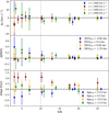 |
Fig. A.1. Recovery of SSP input parameters with PPXF versus S/N of the spectrum. We use four different SSP templates (as indicated by different colours) from the E-MILES library and add artificially Gaussian noise. The noisy spectrum is then fitted with PPXF. For each S/N, we repeat this with five noisy spectra and show the difference between the input parameter and the mean values of these five trails and their standard deviation. The vertical lines indicate the threshold S/N values of ten and three that we chose for reliable measurements of metallicities and velocities, respectively. |
We find that a S/N ≥ 5 is needed to get a radial velocity estimate within 10 km s−1 accuracy. A S/N ≥ 3 is required to get radial velocities within ∼20 km s−1 accuracy. This should be sufficient to determine the velocity dispersion of a large sample of GCs or identifying rotating substructure. Testing with different metallicities, we find that the uncertainties of the radial velocities increase for more metal-poor spectra. This is most likely caused by the lack of strong lines, which makes fitting for the velocity with PPXF’s cross-correlation method more difficult.
We find a S/N ≥ 10 is required to determine the metallicity within 0.2 dex. The age is less well recovered at these low S/N, in particular young ages.
Appendix B: Supplementary information about the dynamical model
In the following, we give additional information about the orbit-based dynamical Schwarzschild model presented in Sect. 7. We present the used MGE model and show the parameter grid of viewing angles as obtained by the model.
B.1. Multi-Gaussian expansion model of FCC 47
We illustrate the MGE model of FCC 47 as used in our Schwarzschild model (Sect. 7) in Fig. B.1. The model is based on a r-band VST image of FCC 47. The original data with some masked sources is shown in black while the contours of the MGE model are overplotted in red.
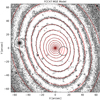 |
Fig. B.1. Illustration of the MGE model of FCC 47 used in our Schwarzschild model. The black contours show the original VST image, the red contours indicate the MGE model. We mask the foreground star close to the galactic centre. |
B.2. Parameter grid of viewing angles
We show the grid of allowed viewing angles θ, ϕ and ψ in Fig. B.2. Each dot corresponds to a single model and the best-fitting model is given by the blue cross. Due to the KDCs in the kinematics, the viewing angles are well constrained and thus only a limited range of deprojections from 2D to 3D are feasible.
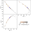 |
Fig. B.2. Parameter grid of allowed viewing angles from our Schwarzschild modelling. The colour and the symbol size give the normalised reduced χ2. The best-fit model is marked by the blue cross. |
Appendix C: Properties of the extracted GCs
We list coordinates, magnitudes, spectral S/N, radial velocities, and – if possible – metallicities of the extracted GCs in Table C.1. The table includes all GCs with S/N ≥ 3.
ID, Coordinates, g-band magnitudes from Jordán et al. (2015) with typical uncertainties of < 0.01 mag, g − z colour, S/N, LOS velocities, and mean metallicities of the GCs in FCC 47.
All Tables
ID, Coordinates, g-band magnitudes from Jordán et al. (2015) with typical uncertainties of < 0.01 mag, g − z colour, S/N, LOS velocities, and mean metallicities of the GCs in FCC 47.
All Figures
|
Fig. 1. Photometric HST/ACS data of FCC 47. Top: HST image of FCC 47 in the F475W filter (roughly g-band). Surface brightness contours from the collapsed MUSE cube (white light image) are superimposed in purple. The levels are logarithmically spaced, but arbitrarly chosen for illustration purposes. Bottom: surface brightness profile of FCC 47 in the F475W filter with a double Sersic profile fit, reproducing the plot from Turner et al. (2012). |
| In the text | |
|
Fig. 2. Distributions of magnitudes and S/N of the extracted GCs. Top: distribution of g-band magnitudes of the GC candidates in the MUSE FOV from Jordán et al. (2015) (blue). The red distribution highlights the GC candidates found in the MUSE data with our method. Bottom: histogram of spectral S/N of the GC candidates and FCC 47-UCD1. |
| In the text | |
|
Fig. 3. Residual image of FCC 47 after subtracting a MGE model of the galaxy. The coloured crosses show the position of GC candidates in the HST catalogue of Jordán et al. (2015), colour-coded by their g-band magnitude. The black circles show the position of 42 GC candidates that are found with the DAOSTARFINDER routine in the MUSE data by cross referencing with the catalogue. The diamond indicates the position of FCC 47-UCD1 with a g-band magnitude of ∼21 mag. The triangles indicate the positions of emission-line background galaxies we found in the MUSE cube. |
| In the text | |
|
Fig. 4. PPXF fit to the background subtracted NSC spectrum. Top: original normalised spectrum is shown in black, the best-fit spectrum in red. For comparison, the spectrum of the local galaxy background is shown in grey. The residual is shown in blue, shifted to 0.6 for visualisation. Masked regions appear as grey shaded. We masked strong sky line residuals as well as the empty region around the sodium D line that is filtered out due to the AO lasers. Bottom: weight maps illustrating the age – metallicity (left), age – [α/Fe] (middle) and [α/Fe] – metallicity (right) grids. The weight of each template used in the fit is given by the greyscale. The black cross shows the weighted mean age, metallicity and α-element abundance with errorbars. The weight maps are normalised. A regularisation parameter of 30 was used in this fit. |
| In the text | |
|
Fig. 5. Stellar light kinematic maps for FCC 47 acquired from the Voronoi-binned MUSE cube. Top left: mean relative velocity of the integrated light with respect to a systemic velocity of 1444 km s−1. Top right: velocity dispersion σ. Bottom left: h3 and bottom right: h4. The inset shows a zoom to the central region to highlight the inner structure. We show the same isophotes as used in Fig. 1. The effective radius of the NSC (0.7″) corresponds to the radius of the innermost isophote contour. |
| In the text | |
|
Fig. 6. Radial profile of LOS velocities of GCs in comparison to the observed scatter in stellar light velocities (green shaded area). The blue shaded area shows the circular velocity profile of FCC 47 as obtained from the orbit-based dynamical model (Sect. 7). The colour of the GCs and FCC 47-UCD1 refers to their (g − z) colour in AB magnitudes taken from Jordán et al. (2015). We show all GCs with S/N > 3 Å−1. The errorbars refer to the 1σ random uncertainty from fitting each GC 300 times. |
| In the text | |
|
Fig. 7. Stellar population maps of FCC 47. Mean ages (left), metallicities [M/H] (middle) and [α/Fe] abundance ratios (right) as determined from a full spectrum fit with PPXF using the alpha-variable MILES template spectra. The maps are mass weighted. We show the same isophotes as in Fig. 1. The inset shows a zoom to the central region and the innermost isophote contour corresponds to the size of the NSC (Reff = 0.7″). |
| In the text | |
|
Fig. 8. Mass weighted, normalised star formation histories of different components of FCC 47. Left: background subtracted NSC in purple, central component in red, the disk in blue and the remaining stellar body in yellow. The dotted lines give the mean ages of each component. The normalisation is chosen such that the weights of each component add up to unity. Right: radial velocity map of FCC 47 as shown in Fig. 5. The black ellipses illustrate how we divided the different components. |
| In the text | |
|
Fig. 9. Radial profile of GC metallicities in comparison to their photometric colours, the NSC, and the integrated galaxy light. Top: radial profile of the mean stellar metallicity (black line) with GCs (circles), UCD (diamond) and the NSC (star). The symbols are colour-coded by their (g − z) colours from Jordán et al. (2015) and Turner et al. (2012). Bottom: (g − z) colours of the photometric sample of GC candidates from Jordán et al. (2015) versus projected distance. The NSC and FCC 47-UCD1 are added and we mark the GCs for which we have spectroscopic metallicity measurements. The dotted line is the mean of GC colours in bins of 10 arcsec. The NSC colour is the colour within a 4-pixel aperture on the HST/ACS images (Turner et al. 2012). We also included the histogram of GC colours to illustrate the bimodal colour distribution. |
| In the text | |
|
Fig. 10. Illustration of the parameter grid explored by our model. Each dot represents one model. The colour code and the symbol size give the reduced |
| In the text | |
|
Fig. 11. Best-fitting Schwarzschild model of FCC 47. Top row: Voronoi binned kinematic data for FCC 47. Left to right: surface brightness, radial velocity and velocity dispersion. Middle row: best-fit Schwarzschild model. Bottom row: residuals created by subtracting the model from the data. The white patches indicate masked bins. The surface brightness counters are taken from the MGE model (see also Fig. B.1). The plotting ranges are not identical to those shown in Fig. 5. |
| In the text | |
|
Fig. 12. Radial profile of enclosed mass and shape parameters. Top: profile of the enclosed mass for the stellar mass (blue), the dark mass (red) and the total (black). Bottom: radial profile of the geometric shape parameters q and p. The dotted lines indicate the 1σ uncertainty determined from the five best-fitting models. |
| In the text | |
|
Fig. 13. Distribution of orbital weights along short axis. Top: circularity λz of the used orbits versus radius. We show a combination of the five best-fitting models. The dotted lines show the effective radius FCC 47 (Reff, FCC 47 = 30″, Ferguson 1989). Bottom: profile of the mass fractions of rotating (yellow), hot (blue) and counter-rotating orbits (red). The solid lines show the combination of the five best-fitting models (dashed lines). |
| In the text | |
|
Fig. 14. Distribution of orbital weights along long axis of the mean of the five best-fitting models. The dotted lines show the effective radius of the NSC (Reff, NSC = 0.7″, Turner et al. 2012) and FCC 47 (Reff, FCC 47 = 30″, Ferguson 1989). The shaded area shows the region where we lack coverage with the MUSE data along the short axis. |
| In the text | |
|
Fig. A.1. Recovery of SSP input parameters with PPXF versus S/N of the spectrum. We use four different SSP templates (as indicated by different colours) from the E-MILES library and add artificially Gaussian noise. The noisy spectrum is then fitted with PPXF. For each S/N, we repeat this with five noisy spectra and show the difference between the input parameter and the mean values of these five trails and their standard deviation. The vertical lines indicate the threshold S/N values of ten and three that we chose for reliable measurements of metallicities and velocities, respectively. |
| In the text | |
|
Fig. B.1. Illustration of the MGE model of FCC 47 used in our Schwarzschild model. The black contours show the original VST image, the red contours indicate the MGE model. We mask the foreground star close to the galactic centre. |
| In the text | |
|
Fig. B.2. Parameter grid of allowed viewing angles from our Schwarzschild modelling. The colour and the symbol size give the normalised reduced χ2. The best-fit model is marked by the blue cross. |
| In the text | |
Current usage metrics show cumulative count of Article Views (full-text article views including HTML views, PDF and ePub downloads, according to the available data) and Abstracts Views on Vision4Press platform.
Data correspond to usage on the plateform after 2015. The current usage metrics is available 48-96 hours after online publication and is updated daily on week days.
Initial download of the metrics may take a while.