| Issue |
A&A
Volume 628, August 2019
|
|
|---|---|---|
| Article Number | A46 | |
| Number of page(s) | 10 | |
| Section | Stellar atmospheres | |
| DOI | https://doi.org/10.1051/0004-6361/201935680 | |
| Published online | 06 August 2019 | |
The CEMP star SDSS J0222–0313: the first evidence of proton ingestion in very low-metallicity AGB stars?★
1
GEPI, Observatoire de Paris, Université PSL, CNRS,
5 place Jules Janssen,
92190
Meudon,
France
e-mail: This email address is being protected from spambots. You need JavaScript enabled to view it.
2
Departamento de Ciencias Fisicas, Universidad Andres Bello,
Fernandez Concha 700,
Las Condes,
Santiago,
Chile
3
Crimean Astrophysical Observatory,
Nauchny
298409,
Republic of Crimea
4
Astronomical Observatory, Odessa National University,
Shevchenko Park,
65014
Odessa,
Ukraine
5
INAF – Osservatorio Astronomico d’Abruzzo,
Via M. Maggini snc,
Teramo,
Italy
6
INFN – Sezione di Perugia,
Via A. Pascoli,
Perugia, Italy
7
European Southern Observatory,
Casilla
19001,
Santiago,
Chile
8
GEPI, Observatoire de Paris, Université PSL, CNRS,
77 Av. Denfert-Rochereau,
75014
Paris,
France
9
INAF – Osservatorio Astronomico di Trieste,
Via G.B. Tiepolo 11,
34143
Trieste,
Italy
10
Dipartimento di Fisica e Astronomia, Università di Firenze,
Via G. Sansone 1,
Sesto Fiorentino,
Italy
Received:
12
April
2019
Accepted:
27
June
2019
Abstract
Context. Carbon-enhanced metal-poor (CEMP) stars are common objects in the metal-poor regime. The lower the metallicity we look at, the larger the fraction of CEMP stars with respect to metal-poor stars with no enhancement in carbon. The chemical pattern of CEMP stars is diversified, strongly suggesting a different origin of the C enhancement in the different types of CEMP stars.
Aims. We selected a CEMP star, SDSS J0222–0313, with a known high carbon abundance and, from a low-resolution analysis, a strong enhancement in neutron-capture elements of the first peak (Sr and Y) and of the second peak (Ba). The peculiarity of this object is a greater overabundance (with respect to iron) of the first s-process peak than the second s-process peak.
Methods. We analysed a high-resolution spectrum obtained with the Mike spectrograph at the Clay Magellan 6.5 m telescope in order to derive the detailed chemical composition of this star.
Results. We confirmed the chemical pattern we expected; we derived abundances for a total of 18 elements and significant upper limits.
Conclusions. We conclude that this star is a carbon-enhanced metal-poor star enriched in elements produced by s-process (CEMP-s), whose enhancement in heavy elements is due to mass transfer from the more evolved companion in its asymptotic giant branch (AGB) phase. The abundances imply that the evolved companion had a low main sequence mass and it suggests that it experienced a proton ingestion episode at the beginning of its AGB phase.
Key words: stars: carbon / stars: abundances / stars: Population II / Galaxy: halo
Based on observations collected with Mike at the Magellan–II (Clay) telescope at the Las Campanas Observatory under programme CN2018B-5.
© E. Caffau et al. 2019
 Open Access article, published by EDP Sciences, under the terms of the Creative Commons Attribution License (http://creativecommons.org/licenses/by/4.0), which permits unrestricted use, distribution, and reproduction in any medium, provided the original work is properly cited.
1 Introduction
Carbon-enhanced metal-poor (CEMP) stars are very common objects in the metal-poor regime ([Fe/H] < −2.0). According to Beers & Christlieb (2005), a metal-poor star can be defined as a CEMP when [C/Fe] > 1.01, and in this work we adopt their definition. Beers & Christlieb (2005) divide CEMP stars into the following sub-classes according to the abundance ratios (implying, besides C, Ba, and Eu): (i) CEMP-r when [C/Fe] > 1.0 and [Eu/Fe] > 1.0. These stars are supposed to be enhanced in heavy elements produced in the rapid n-capture process (r-process); (ii) CEMP-s when [C/Fe] > 1.0, [Ba/Fe] > 1.0, and [Ba/Eu] > 0.5. These stars are expected to be enriched in heavy elements produced in the slow n-capture process (s-process); (iii) CEMP-r/s when [C/Fe] > 1.0 and [Ba/Eu] < 0.5. These stars are characterised by enhancements in all heavy elements; (iv) CEMP-no when [C/Fe] > 1.0 and [Ba/Fe] < 1.0. In principle these stars could show the composition of the cloud where they formed.
More recently, Hansen et al. (2019; see their Table 6) suggested a new classification, efficient in discriminate CEMP-s and CEMP-r, based on the [Sr/Ba] ratio. Both Beers & Christlieb (2005) and Hansen et al. (2019) introduced the sub-classes to all CEMP stars, without a closer look at the C abundance. Their classifications do not subdivide CEMP stars according to the absolute C abundance, A(C)2. Spite et al. (2013) suggested dividing CEMP stars according to their A(C) in a high and a low-carbon band. Later, Bonifacio et al. (2015) suggested a different nature in the C enhancement and the chemical composition of CEMP stars in the two carbon bands. They hypothesised that the stars belonging to the high-carbon band are part of multiple systems, and that their abundance is the result of a mass transfer from the asymptotic giant branch (AGB) phase of the more massive, more evolved companion. These stars also show enhancement in heavy elements (see e.g. Caffau et al. 2018) that put them in the CEMP-s, CEMP-r, or CEMP-r/s sub-classes. Lucatello et al. (2005) and Starkenburg et al. (2014) derived that100% of the CEMP-s stars they investigated show variation in radial velocity, which supports the mass transfer scenario suggested by Bonifacio et al. (2018). The CEMP stars of the low-carbon band, mainly CEMP-no stars according to Bonifacio et al. (2015), can be part of multiple systems (see e.g. Caffau et al. 2016), but their abundances reflect the chemistry of the gas cloud in which they formed. Recently, Arentsen et al. (2019) found four binary systems in a sample of CEMP-no stars, but the fact that some of these stars are binaries is not unexpected.
To understand the early formation and evolution of old, metal-poor stars, it is of invaluable importance to understand the formation of CEMP stars and the mechanism in place that enriched their atmospheres. The majority of the most iron-poor stars known to date are CEMP stars belonging to the low-carbon band described by Spite et al. (2013). The C-rich environment could have made star formation easier (see e.g. Bromm & Loeb 2003). At higher Fe abundance there are stars on both the high-carbon and low-carbon band (see e.g. Caffau et al. 2018), and understanding their composition is extremely important.
We present here the chemical investigation of a Magellan Inamori Kyocera Echelle (Mike) spectrum of SDSS J022226.20–031338.0 (SDSS J0222-0313, for short). We confirm here the abundances derived from a low-resolution FORS spectrum and we increase the number of elements for which we derive the abundance. This is a CEMP star, rich in heavy elements that we classify as a CEMP-s star, according to the scheme of Beers & Christlieb (2005). With its high [Sr/Ba] ratio, according to Hansen et al. (2019) it should be a CEMP-no star, but taking into account the uncertainties in the Sr and Ba determination, it would fit in their CEMP-s sub-class.
2 Selection
The star was selected by Caffau et al. (2018) from the Sloan Digital Sky Survey (SDSS York et al. 2000; Yanny et al. 2009) for its low metallicity and its strong G-band. It was observed on MJD = 57956.32784048 with FORS2 (Appenzeller et al. 1998) at the ESO VLT, in service mode during the ESO programme 088.D-0791. The spectrum was taken with GRISM 1200B, with central wavelength at 436 nm, with 0.′′29 slit width corresponding to a resolving power of 5000 (see Caffau et al. 2018, for details). From the chemical investigation of the FORS spectrum it was clear that the star is a CEMP, with an almost solar carbon abundance, a strong overabundance in Ba ([Ba/Fe] = 1.98) and an even higher overabundance in Sr ([Sr/Fe] = 2.25). Compared to stars in the same metallicity range, enhanced and non-enhanced in carbon, this star occupies an empty region in the [Ba/Fe] versus [Sr/Ba] diagram (see Fig. 1).
3 Observations
We observed SDSS J0222-0313 with the Mike spectrograph (Bernstein et al. 2003) mounted at the Magellan–II (Clay) 6.5 m telescope of the Las Campanas observatory. We used a 0.7′′ slit delivering a resolving power of R = 53 000 and 42 000 on the blue and red side, respectively. We further employed a 2 × 2 on chip binning and fast readout mode. Seven one-hour exposures were taken on the target during the night between October 27 and 28, 2018, under clear sky conditions and seeing variable between 0.7 and 1.0′′. Data were reduced using the CarPy3 python pipeline (Kelson et al. 2000; Kelson 2003). Thorium-argon lamp frames taken during the night were used for the wavelength calibration. Internal quartz lamp frames were used for order localisation, while both quartz frames and observations of the bright B2V star taken with the diffuser into the optical beam (“milky-flat”) were used for flat fielding. Mike spectra cover the wavelength range ≈ 333−506 nm (blue) and ≈ 484−941 nm (red). Individual frames have signal-to-noise ratios (S/N) in the range 20−25 at 400 nm and in the range 30−40 at 780 nm, for all but the last frame of the night which has a significantly lower S/N.
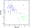 |
Fig. 1 [Ba/Fe] vs. [Sr/Ba] for a sample of metal-poor stars (an updated version of Fig. 1 in Spite et al. 2014). The pink star represents the position of the star J0222–0313 from the analysis of the FORS spectrum (with logg of 4.0; Caffau et al. 2018), while the black star is the result of the investigation of the Mike spectrum, taking into account the NLTE corrections for Sr and Ba. The blue squares are stars from Spite et al. (2005), the green diamonds are CEMP starsfrom the literature (Aoki et al. 2001; Barbuy et al. 2005; Sivarani et al. 2006; Behara et al. 2010; Spite et al. 2013; Yong et al. 2013). The black horizontal dashed line is the r-only solar value for [Sr/Ba] according to Mashonkina & Gehren (2001). Normal stars are in the upper left part of the diagram, sharing the surface with CEMP-no stars; CEMP-s stars are in the lower right part of the diagram. |
4 Analysis
4.1 Radial velocity and kinematics
The radial velocity provided by the Sloan Survey on the SDSS DR12 spectrum is Vr = −124 ± 3 km s−1. We were able to measure the radial velocity from the FORS2 spectrum, Vr = −90 ± 32 km s−1, but due to the flexures of FORS and the lack of telluric absorption in the observed wavelength range, the uncertainty is large. From the Mike spectrum we derived Vr = −127.1 ± 1.2 km s−1 from the cross-correlation of the red Mike spectrum in the spectral range 500–680 nm with a synthetic spectrum computed using the SYNTHE code (Sbordone et al. 2004; Kurucz 2005) along with an ATLAS9 model atmosphere of parameters Teff = 6400 K, log g = 3.00, [Fe/H] = −3 and [α/Fe] = +0.4 and broadened to the resolving power of the Mike spectrum. This radial velocity value takes into account a zero point correction which was calculated by cross-correlating the Mike spectrum with a telluric spectrum calculated with the TAPAS4 (Bertaux et al. 2014) web service for the time and location of the observations and the target coordinates. Cross-correlations were performed using the IRAF5 task fxcor. Even though we expect that the star is in a multiple system, the data at our disposal do not strongly support any binarity information, but we expect the companion to be a low-mass white dwarf (0.5 M⊙), and further investigations would be very useful in order to confirm this binarity.
The parallax for this star in Gaia DR 2 is negative, so we were not able to derive its distance. By using the Gaia colour BP-RP, we compared it to PARSEC isochrones of close metallicity and age of 10.2 Gyr. We ruled out the main sequence solution because the star would have been close enough to allow Gaia to give a parallax and because the dwarf solution is in disagreement with the iron ionisation balance (see next section). We considered the possibility of the star being a sub-giant (log g = 3.8), deriving from the isochrones a distance of 5.4 kpc, and we considered the case of surface gravity derived by matching the Fe abundance from Fe I and Fe II lines, which corresponds to 8.6 kpc (log g = 3.4, assumed in the chemical investigation), respectively. We computed the star’s orbit using the web-based interface GravPot166 (Fernández-Trincado et al. 2016) and in both cases the orbit happens to be a Halo type, with retrograde motion. The star reaches a maximum distance from the Galactic plane of 19 and 39 kpc, respectively. Considering its position in the angular momentum Lz – energy diagram the star could belong to the Sequoia Event recently discovered by Myeong et al. (2019).
4.2 Stellar parameters
Comparing the Gaia photometry to an isochrone, the star could belong to the main sequence (MS), sub-giant (SG), or horizontal branch (HB). Gaia is not able to help us because the parallax value is negative, although Bailer-Jones et al. (2018) provide a distance of 3.0 ± 0.7 kpc assuming anexponential decrease in the Galactic density. At this distance the star should be a MS star, but this is just a statistical result that is not meant to be true for a single star. The MS solution is in disagreement with the chemical investigation and with the fact that at such close distance Gaia would have been able to measure a significant parallax.
We compared the BP-RP Gaia colour to a PARSEC isochrone of metallicity –2.7 and an age of 10.2 Gyr, from Bressan et al. (2012) and (without taking into account any reddening) we derived an effective temperature, Teff, of 6364, 6329, and 6223 K for the three cases of MS, SG, and HB, respectively. Analysing the Mike spectrum with a temperature in this range, the Fe balance is derived in the case close to the SG solution. By fitting Hα wings in the spectral order of the observed Mike spectrum containing Hα, for the five red observations we have for this star, we derive a Teff around 6300 K when the star is a sub-giant, in perfect agreement with the value from the isochrone. Caffau et al. (2018) derived an effective temperatureof Teff = 6345 K from the SDSS photometry. From Gaia BP-RP colour, when applying the reddening from Pan-STARRS (Green et al. 2018)we derive a temperature of 6540 K with the conversion recommended on the PARSEC isochrones site7 ; without reddening we have Teff = 6330 K. The agreement is very close, but we decided to keep the effective temperature of 6345 K from Caffau et al. (2018).
The microturbulence of 1.7 km s−1 was derived from the Fe I lines, as a non-slope of the Fe abundance as a function of the strength of the lines. This microturbulence is consistentwith values derived from high-resolution, high S/N spectra in stars of similar parameters (see e.g. Bonifacio et al. 2009).
We adopted the parameters Teff = 6345 K, log g = 3.4 and ξ = 1.7 km s−1, and we derived [Fe/H] = –2.82. The uncertainties we associated with the stellar parameters are 100 K for the effective temperature, 0.4 dex for the surface gravity, and 0.2 km s−1 for the microturbulence. The uncertainty of 100 K in Teff is that derived fromthe fit on the wings of Hα; we recall that this temperature and the one derived from the Gaia DR2 colour are in very good agreement. For the gravity, a 0.4 dex uncertainty allows the star to be an SG or an HB star. For the microturbulence, we would not expect a microturbulence smaller than 1.5 km s−1 for an evolved star, nor larger than 1.8 km s−1 for a warm star. With these parameters the star does not fit in the PARSEC isochrone of the metallicity of the star. A surface gravity of 3.8 would put the star in the SG branch of the PARSEC isochrone (see Fig. 2). This value of gravity would keep the Fe abundances from the Fe I and Fe II lines still compatible within uncertainties. A difference of 0.4 dex in the surface gravity does not change the chemical inventory of the star. For the SG solution, according to the isochrone, the star has a mass of M = 0.8 M⊙.
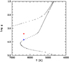 |
Fig. 2 PARSEC isochrone for [M/H] = –2.75 and an age of 10.2 Gyr (small black dots) (from Bressan et al. 2012). The red symbol shows the parameters we derived (Teff from the SDSS photometry and logg from the Fe ionisation equilibrium). The blue symbol on the isochrone corresponds to a log g that is 0.4 dex higher and corresponds to a disagreement in A(Fe) of 0.13 dex between the abundance derived from Fe I lines and that derived from Fe II lines. This value is well within the uncertainties. |
Chemical abundances.
4.3 Abundances
The spectrum was analysed with MyGIsFOS (see Sbordone et al. 2014), an automatic code able to derive chemical abundances by comparing an observed spectrum to a grid of synthetic spectra. We computed the synthetic spectra with the code SYNTHE (see Kurucz 2005; Sbordone et al. 2004) from a grid of ATLAS 12 model (Kurucz 2005). With MyGIsFOS we derived the abundances for Mg, Ca, Sc, Ti, Cr, Mn, Fe, Co, and Ni. For the other elements we computed an ATLAS 12 model with the stellar parameters of the star and an enhancement in Mg, C, and O, as we derived from the analysis, and the nitrogen (which we could not derive) enhanced as much as the carbon. From this model we computed with SYNTHE a grid of synthetic spectra with different abundances of the elements to be derived. We compared the observed spectrum to the grid of synthetic spectra and performed a χ2 minimisation to derive the abundances.
For oxygen we measured the equivalent widths of the three lines of the triplet at 777 nm and, by using WIDTH (Kurucz 2005), we derived the oxygen abundance. For carbon we fitted the G-band and also six atomic lines visible in the Mike spectrum, thanks to the high C in this star. The A(C) derived from the G-band is in good agreement with the abundance derived from the C I line after applying the non-local thermodynamic equilibrium (NLTE) correction. From the G-band, by fitting the range 422.9–423.2 nm, we also derived the isotopic ratio 12C /13C as 7.4 ± 1.5, where the uncertainty is the formal 1σ provided by the χ2 fitting. The abundances we derived are listed in Table 1.
We havea tentative detection of Th from the 401.9 nm Th II line. The measurement is uncertain and is shown in Fig. 3. This line is blended with a 13CH line, which is taken into account in the fit of the Th line, with 12C /13C = 7.4. The presence of this feature at the wavelength of the Th II line could be explained with a low 12C /13C ratio of 5 ± 1.5, but this value is only marginally consistent with the result from the CH line at 423 nm (see Fig. 4). We searched for U, but due to the relatively low S/N in this range, we cannot measure but nor do we rule out the presence of the 385.9 nm U II line in the spectrum (see Fig. 5).
The abundances with respect to iron, [X/Fe], and the upper limits are summarised in Fig. 6. Figure 7 shows the abundances with respect to yttrium, [X/Y ], of the heavyelements, highlighting a peculiar chemical pattern of this star.
4.4 NLTE computations
Atomic levelpopulations for all studied atoms were determined using the MULTI code (Carlsson 1988) with modifications as given in Korotin et al. (1999). Proper comparison of observed and computed profiles in many cases requires a multi-element synthesis to take into account possible blending lines of other species. For this process we fold the NLTE (MULTI) calculations,specifically the departure coefficients, into the LTE synthetic spectrum code SYNTHV (Tsymbal 1996), which enables us to calculate the NLTE source function for lines of the chemical element under consideration. These calculations included all spectral lines from the VALD data base (Ryabchikova et al. 2015) in a region of interest. The LTE approach was applied for lines other than the lines of the chemical element under consideration. Abundances of corresponding elements were adopted in accordance with the [Fe/H] value.
The NLTE corrections for all the atomic lines of C, O, Na, Mg, Al, Ca, Sr, and Ba were determined, and in Table 1 the NLTE corrections and the abundances after applying the NLTE corrections are provided. For carbon, we used the atomic model described in Lyubimkov et al. (2015). The model consists of 47 levels of C I, 11 levels of C II, and the ground levelof C III. In addition, we included in the model 63 levels of C I and 9 levels of C II in order to calculate partition function in LTE. A total of 207 radiative transitions were considered in detail. For 128 weak b–b transitions, radiative rates were considered in LTE. They were unchanged in calculations of the NLTE level populations. There is a remarkable difference inNLTE corrections between the lines of different multiplets for the neutral carbon. The lines in the optical domain are practically formed in LTE, and their NLTE corrections are small (they do not usually exceed − 0.1 dex). The situation with lines in the IR region is the opposite. This is visible from the line-to-line scatter, which is definitely smaller after applying the NLTE corrections. The NLTE effects lead to a significant amplification of the profiles (corrections achieve − 0.6 dex).
The NLTE model of the oxygen atom was first described by Mishenina et al. (2000), and then updated by Korotin et al. (2014). The model consists of 51 O I levels of singlet, triplet, and quintet systems, and the ground level of the O II ion. An additional 24 levels of neutral oxygen and 15 levels of ions in higher states were added for particle number conservation. Fine structure splitting was taken into account only for the ground level and the 3p5P level (the upper level of the triplet lines at 777 nm). A total of 248 bound–bound transitions were included. Accurate quantum mechanical calculations were employed for the first 19 levels to find collision rates with electrons (Barklem 2007).
The NLTE atomic model of sodium was presented by Korotin et al. (1999) and then updated by Dobrovolskas et al. (2014). The updated sodium model currently consists of twenty energy levels of Na I and the ground level of Na II. In total, 46 radiative transitions were taken into account for the calculation of the population of all levels. Fine structure splitting was taken into account only for the 3p level to ensure reliable calculations of the D line profiles. Collisional cross-sections obtained using quantum mechanical computations (Barklem et al. 2010) were used for the nine lowest levels. For other levels, the classical formula of Drawin was utilised in the form suggested by Steenbock & Holweger (1984), with the correction factor SH = 1∕3. The NLTE effects strengthen the sodium lines.
In the case of Mg, we used the model atom from Mishenina et al. (2004). It consisted of 84 levels of Mg I, 12 levels of Mg II, and the ground state of Mg III. In the computation of departure coefficients, radiative transitions between the first 59 levels of Mg I and the ground level of Mg II were taken into account. All 424 b–b transitions were included in the linearisation procedure. The model then was modified by Černiauskas et al. (2017), who added collisional rates with hydrogen atoms for transitions between the eight lower levels (Barklem et al. 2012). From the ADAS database8 effective collision strengths with electrons were taken for the transition between the 13 lower levels. This modified model was tested with the help of the solar spectrum, Procyon spectrum and spectra of three stars with metal deficiency: HD 211998 ([Fe/H] = –1.6), HD 140283 ([Fe/H] = −2.5), and HD 122563([Fe/H] = –2.7). The magnesium lines we analysed have NLTE corrections that are rather small. They have different signs and do not exceed 0.10 dex.
The Al atomic model is described in detail in Andrievsky et al. (2008). This model atom consists of 76 levels of Al I and 13 levels of Al II. The model was modified to some extent. First we added collisional rates with hydrogen atoms for transition between several lower levels (Belyaev 2013). Similarly to the magnesium model, we also used spectra of several stars to test the aluminium atomic model. The spectra of the following stars were used: the Sun, Arcturus, Pollux, HR4796, Procyon, and Canopus. Comparison of observed and synthesised profiles of lines from different multiplets show good agreement, and this confirms the reliability of our aluminium model. Unfortunately in our spectroscopic analysis of SDSS J0222–0313 we were limited by only one available Al I line at 396 nm strongly affected by NLTE, which translates into a large NLTE correction (see Table 1).
The calcium abundance was derived by analysis of calcium lines in the two ionisation states. Our model of Ca atom consists of 70 levels of Ca I, 38 levels of Ca II, and the ground state of Ca III. In addition, more than 300 levels of Ca I and Ca II were included to keep the condition of the particle number conservation in LTE. The information about the adopted oscillator strengths, photoionisation cross-sections, collisional rates, and broadening parameters can be found in Spite et al. (2012). This model was modified later on and collisional rates between calcium and hydrogen atoms for the 20 lower levels of Ca I were added. The necessary data were taken from Belyaev et al. (2017). Similar to the atomic model of magnesium and aluminium, our Ca models were tested with the help of the spectra of well-studied stars: the Sun, Arcturus, Pollux, and Procyon.
The strontium atomic model includes 44 low levels of Sr II with n ≤12 and l ≤ 4 and the ground level of Sr III. It also accounts for the fine splitting under the terms 4d2D and 5p2P0, which is why we included 24 Sr I levels only in the equation of particle number conservation. A more detailed description of the model atom can be found in Andrievsky et al. (2011).
The barium model contains 31 levels of Ba I, 101 levels of Ba II with n ≤50, and the ground level of Ba III. The 91 b–b transitions between the first 28 levels of Ba II (n ≤ 12 and l < 5) were also computed in detail. For two levels, 5d2D and 6p2P0, the fine structure was taken into account. The odd Ba isotopes have hyperfine splitting of their levels, and thus several hyperfine structure components for each line (Rutten 1978). This effect is most pronounced for the Ba II lines 455.4 and 649.6 nm. The information about the adopted oscillator strengths, photoionisation cross-sections, collisional rates and broadening parameters can be found in Andrievsky et al. (2009). In the spectrum of our programme star, two resonance lines (455.4 and 493.4 nm), and one subordinate line (614.1 nm) were analysed.
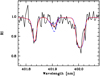 |
Fig. 3 Observed spectrum (solid black) in the range of the 401.9 nm Th II line, compared with the best fit (solid red) providing A(Th) = 0.12, and two synthetic spectra at A(Th) of − 0.3 and 0.5 (dashed blue). The Th II line is blended with a 13CH line, which is taken into account. |
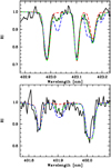 |
Fig. 4 Top panel: observed spectrum (solid black) in the range of the G-band, compared with synthetic spectra with different 12C/13C ratios (dashed red 90; dashed green 7.5, the best fit; and dashed blue 3). Bottom panel: Th II line with the synthetic spectra of the top panel and with a solar scaled Th abundance. |
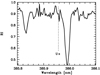 |
Fig. 5 Observed spectrum (solid black) in the range of the 385.9 nm U II line. |
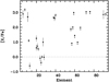 |
Fig. 6 Abundances with respect to iron that we derived for this star. |
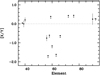 |
Fig. 7 Abundances of the heavy elements with respect to Y that we derived for this star. |
4.5 Uncertainties
The uncertainties reported in Table 1 are the line-to-line scatter for both the LTE and NLTE analysis. When the abundance was derived from one single line or the G-band we looked at the uncertainty in the determination of the continuum and the S/N to estimate the error. These uncertainties are reported in the figures. In Table 2 we list the systematic uncertainties related to the uncertainties in the stellar parameters. The uncertainty on the [Sr/Ba] ratio is not very affected by the uncertainties on the stellar parameters because they react in a similar way as a consequence of changes in the stellar parameters.
Variations in the chemical abundances related to changes in the stellar parameters.
5 Discussion
SDSS J0222–0313 is characterised by a high C abundance that places the star on the high-carbon band as defined by Spite et al. (2013) and Bonifacio et al. (2015, see their Fig. 6). In Fig. 8 we present a revisit on this plot with SDSS J0222–0313 depicted as a red starsymbol. Its C abundance (A(C) = 8.45) is even higher than the value we derived from the low-resolution spectrum in Caffau et al. (2018). In that paper we concluded that the stars in the high-carbon band, which showed a systematic enhancement in Ba, belong to multiple systems and that their chemical composition has been altered by a more evolved companion, while the stars in the low-carbon band, with a normal Ba abundance, have a chemical composition of the gas cloud in which they formed.
In Fig. 9, we compared the abundances of C, O, Sr, and Ba with respect to Fe derived for SDSS J0222–0313 with stars analysed by Hansen et al. (2016a, 2019), which are mostly CEMP stars. SDSS J0222–0313 is always in the upper part of each panel, but still consistent with the comparison sample stars.
SDSS J0222–0313 is rich in Ba (i.e. [Ba/Fe] > 1) with [Ba/Fe] = +1.86 in LTE; it is also rich in Sr with [Sr/Fe] = +2.66 in LTE, and has a significant upper limit in Eu ([Eu/Fe] < −1.0). The star is rich in heavy elements produced mainly during s-process (Sr peak and Ba peak), but not in elements produced mainly during r-process. It also belongs to the high-carbon band, so SDSS J0222–0313 could be classified as a CEMP-s star. However, it shows at least two chemical features that are rather peculiar for a CEMP-s star. The first is the very high ratio of [Sr/Ba] = 0.80 in LTE, which cannot be reproduced by a standard s-process nucleosynthesis in AGB stars at low metallicities (Bisterzo et al. 2012). We note that even low-metallicity massive AGB stars, whose heavy element nucleosynthesis may be dominated by the 22Ne(α,n)25Mg reaction (which tends to produce more low-mass s-elements, ls, than high-mass s-elements, hs), are not able to fit the spectrum observed in SDSS J0222–0313 (see e.g. Cristallo et al. 2015). This ratio would place this star in the CEMP-no area, according to the classification of Hansen et al. (2019, see Fig. 10), but SDSS J0222–0313 is clearly too rich in Ba and Sr to be a CEMP-no star. This misclassification, still compatible with the classification by Hansen et al. (2019) within the uncertainties, is a clear symptom that this star has an uncommon chemical pattern. The s-process nucleosynthesis in rotating massive stars is able to produce this level of [Sr/Ba] ratio (Frischknecht et al. 2016; Limongi & Chieffi 2018), but rotating massive stars eject Sr and Ba only during supernovae explosion. For this reason, a mass transfer should be excluded in this scenario (but see Choplin et al. 2017). Chemical evolution models with rotating massive stars fail to reproduce the almost solar A(C) value (Cescutti et al. 2016) and enhancement of strontium and barium (Cescutti et al. 2013). Furthermore, cosmological chemical evolution models for the formation of the Milky Way predict that CEMP stars should have [C/Fe] < 2.0 at [Fe/H] > −3 if they are enriched by primordial faint supernovae (see e.g. Fig. 8 in de Bennassuti et al. 2017), which can be produced by fast-rotating massive stars (e.g. Meynet et al. 2006). We can thus exclude this scenario since SDSS J0222–0313 has [C/Fe] = +2.73 and [Fe/H] = −2.82. In addition, SDSS J0222–0313 has a second peculiarity. This star actually has an extremely low abundance of lanthanum compared to that of barium: the upper limit on lanthanum ([La/Fe] < 0.92) is basically 1dex below the [Ba/Fe] ratio. Neither standard s-process nucleosynthesis in AGB stars nor s-process nucleosynthesis in rotating massive stars can reproduce this 1 dex difference between these two elements.
It is well known that, at very low metallicities, a sub-sample of CEMP stars show surface distributions enriched in both s- and r-process elements (the so-called CEMP-rs stars). Even if these objects are characterised by very high [hs/ls] ratios (thus at odds with SDSS J0222–0313), it may be worth considering their pollution history. One of the most popular explanations ascribes these exotic distributions to a nucleosynthesis process, halfway between thes-process and r-process: the so-called intermediate process (i-process, characterised by neutron densities nn ~ 1014 ÷ 1016 cm−3; Cowan & Rose 1977). The stellar site(s) where the i-process is at work has(have) not been univocally identified yet. To date, the most promising candidates are rapidly accreting white dwarfs (RAWDs) and proton ingestions in low-mass low-metallicity stars.
Denissenkov et al. (2017) have proposed RAWDs in close binary systems as an astrophysical site for the i-process. They concluded that these objects are an important site for the Galactic production of elements belonging to the first-peak of the s-process (comparable to low-mass AGB stars). RAWDs are able to reproduce the surface heavy element distribution of Sakurai objects (characterised by almost solar metallicities; see Herwig et al. 2011). However, at low metallicities these objects produce more heavy s-elements than light s-elements (see e.g. Fig. 11 of Denissenkov et al. 2018). Thus, we discard this possibility to explain the abundances observed in SDSS J0222–0313 (which has a very low [hs/ls] ratio).
In recent years, one-zone post-process calculations for the i-process have become available (Dardelet et al. 2014; Hampel et al. 2016). These calculations are characterised by very high neutron densities (nn > 1015 cm−3) and, as a consequence, show high [Ba/La] and [hs/ls] ratios. While the first ratio closely agrees with the spectrum observed in SDSS 0222–0313, the second clashes with the low measured [hs/ls]. These theoretical explorations do not anchor the occurrence of the i-process to a specific stellar site.
A promising physical process to produce the abundance pattern as observed in SDSS 0222–0313 is the ingestion of hydrogen in a convectively unstable He-burning region (hereafter proton ingestion episode, PIE). Such a peculiar mixing episode strongly depends on the stellar mass and metallicity: the lower the two quantities, the higher the probability of having a PIE (with an increasingly higher efficiency). There is a vast amount of literature on PIEs, which may occur during off-centre He-burning flashes (before core He-burning at extremely low metallicities) or at the first fully developed thermal pulse at slightly higher Z (Hollowell et al. 1990; Fujimoto et al. 2000; Iwamoto et al. 2004; Campbell & Lattanzio 2008; Cristallo et al. 2009, 2016; Koch et al. 2019). As a general rule, these models show [hs/ls] not compatible (i.e. too high) with SDSS J0222–0313. Nevertheless, hints that both these conditions are satisfied can be found in the model published by Cristallo et al. (2009), i.e. a 1.5 M⊙ model at [Fe/H] = –2.44 with no alpha-element enrichment ([α/Fe] = 0)9.
In this model, at the time of the first fully developed thermal pulse (TP), some protons are engulfed in the growing convective shell triggered by the sudden activation of the 3α process. This occurs because the entropy barrier supported by the hydrogen-burning shell is small, due to the rather low CNO abundance in the envelope. As soon as protons are mixed within the shell, they are mixed downward and burn on-the-fly. Cristallo et al. (2009) calculated them by setting appropriate limits to the mixing of protons, which take into account the ratio between the mixing turnover timescale and the local proton burning timescale. Thus, protons are mixed down to a fixed mass coordinate, locally releasing a large amount of energy. On the other hand, H-burning products (in particular 13C and 14N) are mixed down to the bottom of the convective shell, where the temperature largely exceeds 100 MK and the 13C(α,n)16O is efficiently activated. As a consequence, a rich s-process nucleosynthesis develops (see Fig. 5 of Cristallo et al. 2009). When the energy released by the H-burning exceeds the energy produced at the bottom of the shell, the convective shell splits, and the two sub-shells experience a completely different nucleosynthesis. In particular, the upper shell continues to ingest protons, thus further synthesising 13C, which burns at a lower temperature and thus is only able to feed the first s-process peak (Sr-Y-Zr). Later, the envelope penetrates downwards (third dredge-up, TDU), mixing the whole upper shell within the envelope, which results strongly enriched in light s-elements only (see Fig. 6 of Cristallo et al. 2009).
Actually, we also expect the envelope to be slightly Ba-rich. This derives from the fact that, during a PIE, a large amount of 135I is produced, which later decays to 135Cs (τ ~ 9 h), and finally to 135Ba (τ ~ 2 × 10⁶ yr). This is a consequence of the extremely high neutron densities attained by the model (nn > 1014 cm−3). Moreover, this model predicts a very low envelope 12C/13C ratio (less than 10) and large overabundances of 14N (from H-burning) and 16O (coming from the 13C(α,n)16O reaction).
A number of points, however, deserve to be discussed in more detail. First, it should be noted that the model presented by Cristallo et al. (2009) and the subsequent set published in Cristallo et al. (2016) experience further normal TPs followed by efficient TDUs. These TDUs smooth or even erase the nucleosynthesis features characterising the first TDU. Actually, the model presented in Cristallo et al. (2009) has [Fe/H] = –2.45 and [α/Fe] = 0, while the models published in Cristallo et al. (2016) were computed with an initial [Fe/H] = –2.85 and an α enrichment [α/Fe] = 0.5 (i.e. the value characterising halo stars, on average). The global metallicities of the two sets are equivalent (Z ~ 5 × 10⁻⁵), but they have a completely different relative element distribution. The inclusion of an α enhancement strongly influences the nucleosynthesis triggered by the PIE. As a net result, the 1.5 M⊙ model in Cristallo et al. (2016) shows a large [hs/ls] already at the first TDU. In fact, an increase in the oxygen abundance (as in the α-enhanced case) delaysthe occurrence of the shell splitting. On the other hand, SDSS J0222–0313 shows an α-rich spectrum, and thus we cannot ignore it. However, one additional thought should be given to the treatment of these peculiar processes in hydrostatic 1D models. During a PIE, the nuclear energy released within the convective turnover timescale is coupled to the turbulent mixing, which occurs on different length scales. Therefore, average quantities (as calculated in 1D codes) may not be representative of the real processes occurring in stars. In the past, there have been attempts to simulate these mixing events with 3D simulations (Mocák et al. 2010; Stancliffe et al. 2011; Herwig et al. 2014; Woodward et al. 2015). However, the details (and results) of the available simulations differ widely. Moreover, current simulations are strongly dependent on the adopted resolution. As a consequence, the current available hydrodynamic 3D simulations are not ready to efficiently (and firmly) constrain the physics and nucleosynthesis of PIEs yet. Some of these 3D models, however, show that some material is mixed through the hydrogen burning region, thus relaxing the assumption that protons can only be mixed down to a well-defined layer (as done in Cristallo et al. 2009, 2016 models).
Another important point to be discussed is the effect that a PIE would have on models with an initial mass M ≤ 1 M⊙. For these low masses, we expect that the occurrence of the PIE may trigger a dynamical expulsion of the whole envelope, due to the sudden release of energy by CNO burning at the base of the upper shell. This would avoid any further mixing in the envelope, thus preserving the PIE features in the material lost. When this material is accreted by a companion star, the nucleosynthetic pattern is fully preserved.
Far from concluding that the uncommon heavy element distribution of SDSS J0222–0313 is unequivocally ascribed to a PIE, we guess that a very low-metallicity model ([Fe/H] ~−2.85) with a low initial mass (M ≤ 0.9 M⊙) may closely reproduce all the observed features. We reserve the calculation of this model and the exploration of the adopted physical prescriptions to a future paper, but it is worthwhile to discuss this scenario. In this hypothetical binary system, the difference in mass between SDSS J0222–0313 and the more evolved companion would be small. According to the PARSEC isochrone, SDSS J0222–0313 has a mass of about 0.8 M⊙. If the primary companion of the system has a slightly higher mass (e.g. M ~ 0.9 M⊙), it would arrive on the AGB with a tiny envelope (due to the mass lost during the red giant branch phase). In the case of a dynamical expulsion of the whole envelope, it would be plausible to have a consistent fraction of material accreted on the secondary companion. At that epoch, this secondary companion would still be in the main sequence phase and its envelope would be radiative. As a consequence, the accreted material would not need any dilution, apart from secular effects due to the gravitational settling for example; however, they are hard to predict a priori (see e.g. Stancliffe 2010).
The fact that no other star with a chemical pattern like that of SDSS J0222–0313 has yet been found, may be also due to a lower probability of forming stars with similar masses in binary systems than with a large difference in masses. The distribution of the mass ratio10 for solar metallicity stars peaks at about q = 0.25 (Duquennoy & Mayor 1991), while theoretically for Pop III stars it should be even more biased towards very low mass ratios (Stacy & Bromm 2013). The fact that we do not see variations in the radial velocity of SDSS J0222–0313 can be attributed to too few secured spectra, or spectra acquired at the wrong time.
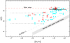 |
Fig. 8 A(C) vs. [Fe/H] for known CEMP stars (from Spite et al. 2013). SDSS J0222–0313 (red star) is compared to the CEMP sample stars (open red bullets) analysed in our collaboration (Bonifacio et al. 2015, 2018, 2009; Caffau et al. 2016, 2013; Sivarani et al. 2006, 2004; Spite et al. 2013; Behara et al. 2010) and unevolved CEMP stars (light blue square) and evolved CEMP stars (double light blue squares) from the literature (Yong et al. 2013; Cohen et al. 2003, 2013; Carollo et al. 2014; Masseron et al. 2012; Jonsell et al. 2006; Thompson et al. 2008; Hansen et al. 2015, 2016b; Lucatello et al. 2003; Aoki et al. 2002, 2006, 2008; Frebel et al. 2005, 2015; Li et al. 2015; Norris et al. 2007; Christlieb et al. 2004; Keller et al. 2014; Roederer et al. 2014; Ivans et al. 2005). |
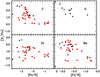 |
Fig. 9 Abundances of the SDSS J0222–0313 in LTE (blue star) compared to the CEMP sample from Hansen et al. (2016a; black diamonds) and Hansen et al. (2019; red squares). |
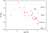 |
Fig. 10 [Sr/Ba] ratio of SDSS J0222–0313 (blue star for the LTE ratio and open circle for the NLTE value) compared to the CEMP sample from Hansen et al. (2016a, black diamonds) and Hansen et al. (2019, red squares), with [Fe/H ] < −2.0. Error bars for SDSS J0222–0313 are the uncertainties in [Ba/Fe] and [Sr/Ba]. We include the division (dotted lines) suggested by Hansen et al. (2019) in their Fig. 7. The star SDSS J0222–0313, being a CEMP-s star, would be expected to have a lower [Sr/Ba] value due to its high [Ba/Fe]. |
6 Conclusions
SDSS J0222–0313 is a halo star with a retrograde orbit, compatible with the Sequoia accretion event described by Myeong et al. (2019). It is a CEMP star belonging to the high-carbon band described by Spite et al. (2013), with an almost solar C abundance and a low 12C/13C ratio of 7.4. Its atmosphere is also enriched in neutron-capture elements of the first peak and in Ba. Its chemical compositioncould be explained by mass transfer from a more evolved low-mass companion in its AGB phase. The conditions for the more evolved companion to discharge on its atmosphere n-capture elements of the first peak and not of the second peak can be due to a quite rare case of proton ingestion episode, as described by Cristallo et al. (2009). No variation in radial velocity is clearly evident from the acquired spectra to confirm that the star has a companion. The low mass of the white dwarf companion would change the radial velocity by a small quantity, but we can also be dealing with a pole-on system, for which we could never detect variation in radial velocity. We will try to secure further spectra in the future in order to have more radial velocity measurements to see if we are able to derive the orbit of the system and so the mass ratio. These high-resolution spectra would also allow us to determine the odd-to-even ratio of barium isotopes, thus supporting or discarding the hypothesis that the chemical distribution of this star is a fingerprint of a proton ingestion episode (which predicts a large enhancement of 135Ba with respect to 138Ba, the most abundant isotope in normal s-process enriched stars).
With all their limitations, classifications of CEMP stars are very useful to place stars with similar chemical properties in the same sub-class; for example, the Spite et al. (2013) division in A(C) is very useful for distinguishing CEMP-no from other CEMP stars. With the classification by Hansen et al. (2019) we can quite confidently separate a CEMP-s from a CEMP-r star. But these classificaitons can also be used to help recognise strange objects, which can be identified by their misfits.
Acknowledgements
E.C. and P.B. have been supported by the Programme National de Physique Stellaire of the Institut National des Sciences de l’Univers of CNRS. This work has made use of data from the European Space Agency (ESA) mission Gaia (https://www.cosmos.esa.int/gaia), processed by the Gaia Data Processing and Analysis Consortium (DPAC, https://www.cosmos.esa.int/web/gaia/dpac/consortium). Funding for the DPAC has been provided by national institutions, in particular the institutions participating in the Gaia Multilateral Agreement.
References
- Andrievsky, S. M., Spite, M., Korotin, S. A., et al. 2008, A&A, 481, 481 [NASA ADS] [CrossRef] [EDP Sciences] [Google Scholar]
- Andrievsky, S. M., Spite, M., Korotin, S. A., et al. 2009, A&A, 494, 1083 [NASA ADS] [CrossRef] [EDP Sciences] [Google Scholar]
- Andrievsky, S. M., Spite, F., Korotin, S. A., et al. 2011, A&A, 530, A105 [NASA ADS] [CrossRef] [EDP Sciences] [Google Scholar]
- Aoki, W., Ryan, S. G., Norris, J. E., et al. 2001, ApJ, 561, 346 [NASA ADS] [CrossRef] [Google Scholar]
- Aoki, W., Ryan, S. G., Norris, J. E., et al. 2002, ApJ, 580, 1149 [NASA ADS] [CrossRef] [Google Scholar]
- Aoki, W., Frebel, A., Christlieb, N., et al. 2006, ApJ, 639, 897 [NASA ADS] [CrossRef] [Google Scholar]
- Aoki, W., Beers, T. C., Sivarani, T., et al. 2008, ApJ, 678, 1351 [NASA ADS] [CrossRef] [Google Scholar]
- Appenzeller, I., Fricke, K., Fürtig, W., et al. 1998, The Messenger, 94, 1 [NASA ADS] [Google Scholar]
- Arentsen, A., Starkenburg, E., Shetrone, M. D., et al. 2019, A&A, 621, A108 [NASA ADS] [CrossRef] [EDP Sciences] [Google Scholar]
- Bailer-Jones, C. A. L., Rybizki, J., Fouesneau, M., Mantelet, G., & Andrae, R. 2018, AJ, 156, 5 [CrossRef] [Google Scholar]
- Barbuy, B., Spite, M., Spite, F., et al. 2005, A&A, 429, 1031 [NASA ADS] [CrossRef] [EDP Sciences] [Google Scholar]
- Barklem, P. S. 2007, A&A, 462, 781 [NASA ADS] [CrossRef] [EDP Sciences] [Google Scholar]
- Barklem, P. S., Belyaev, A. K., Dickinson, A. S., & Gadéa, F. X. 2010, A&A, 519, A20 [NASA ADS] [CrossRef] [EDP Sciences] [Google Scholar]
- Barklem, P. S., Belyaev, A. K., Spielfiedel, A., Guitou, M., & Feautrier, N. 2012, A&A, 541, A80 [NASA ADS] [CrossRef] [EDP Sciences] [Google Scholar]
- Beers, T. C., & Christlieb, N. 2005, ARA&A, 43, 531 [NASA ADS] [CrossRef] [Google Scholar]
- Behara, N. T., Bonifacio, P., Ludwig, H.-G., et al. 2010, A&A, 513, A72 [NASA ADS] [CrossRef] [EDP Sciences] [Google Scholar]
- Belyaev, A. K. 2013, A&A, 560, A60 [NASA ADS] [CrossRef] [EDP Sciences] [Google Scholar]
- Belyaev, A. K., Voronov, Y. V., Yakovleva, S. A., et al. 2017, ApJ, 851, 59 [NASA ADS] [CrossRef] [Google Scholar]
- Bernstein, R., Shectman, S. A., Gunnels, S. M., Mochnacki, S., & Athey, A. E. 2003, Proc. SPIE, 4841, 1694 [NASA ADS] [CrossRef] [Google Scholar]
- Bertaux, J. L., Lallement, R., Ferron, S., Boonne, C., & Bodichon, R. 2014, A&A, 564, A46 [NASA ADS] [CrossRef] [EDP Sciences] [Google Scholar]
- Bisterzo, S., Gallino, R., Straniero, O., Cristallo, S., & Käppeler, F. 2012, MNRAS, 422, 849 [NASA ADS] [CrossRef] [Google Scholar]
- Bonifacio, P., Caffau, E., Spite, M., et al. 2009, A&A, 501, 519 [NASA ADS] [CrossRef] [EDP Sciences] [Google Scholar]
- Bonifacio, P., Caffau, E., Spite, M., et al. 2015, A&A, 579, A28 [NASA ADS] [CrossRef] [EDP Sciences] [Google Scholar]
- Bonifacio, P., Caffau, E., Spite, M., et al. 2018, A&A, 612, A65 [NASA ADS] [CrossRef] [EDP Sciences] [Google Scholar]
- Bressan, A., Marigo, P., Girardi, L., et al. 2012, MNRAS, 427, 127 [NASA ADS] [CrossRef] [Google Scholar]
- Bromm, V., & Loeb, A. 2003, Nature, 425, 812 [NASA ADS] [CrossRef] [EDP Sciences] [PubMed] [Google Scholar]
- Caffau, E., Ludwig, H.-G., Steffen, M., Freytag, B., & Bonifacio, P. 2011, Sol. Phys., 268, 255 [NASA ADS] [CrossRef] [Google Scholar]
- Caffau, E., Bonifacio, P., François, P., et al. 2013, A&A, 560, A15 [NASA ADS] [CrossRef] [EDP Sciences] [Google Scholar]
- Caffau, E., Bonifacio, P., Spite, M., et al. 2016, A&A, 595, L6 [Google Scholar]
- Caffau, E., Gallagher, A. J., Bonifacio, P., et al. 2018, A&A, 614, A68 [NASA ADS] [CrossRef] [EDP Sciences] [Google Scholar]
- Campbell, S. W., & Lattanzio, J. C. 2008, A&A, 490, 769 [NASA ADS] [CrossRef] [EDP Sciences] [Google Scholar]
- Carlsson, J. 1988, Phys. Rev. A, 38, 1702 [NASA ADS] [CrossRef] [Google Scholar]
- Carollo, D., Freeman, K., Beers, T. C., et al. 2014, ApJ, 788, 180 [NASA ADS] [CrossRef] [Google Scholar]
- Černiauskas, A., Kučinskas, A., Klevas, J., et al. 2017, A&A, 604, A35 [NASA ADS] [CrossRef] [EDP Sciences] [Google Scholar]
- Cescutti, G., Chiappini, C., Hirschi, R., Meynet, G., & Frischknecht, U. 2013, A&A, 553, A51 [NASA ADS] [CrossRef] [EDP Sciences] [Google Scholar]
- Cescutti, G., Valentini, M., François, P., et al. 2016, A&A, 595, A91 [NASA ADS] [CrossRef] [EDP Sciences] [Google Scholar]
- Choplin, A., Hirschi, R., Meynet, G., & Ekström, S. 2017, A&A, 607, L3 [NASA ADS] [CrossRef] [EDP Sciences] [Google Scholar]
- Christlieb, N., Gustafsson, B., Korn, A. J., et al. 2004, ApJ, 603, 708 [NASA ADS] [CrossRef] [Google Scholar]
- Cohen, J. G., Christlieb, N., Qian, Y.-Z., & Wasserburg, G. J. 2003, ApJ, 588, 1082 [NASA ADS] [CrossRef] [Google Scholar]
- Cohen, J. G., Christlieb, N., Thompson, I., et al. 2013, ApJ, 778, 56 [NASA ADS] [CrossRef] [Google Scholar]
- Cowan, J. J., & Rose, W. K. 1977, ApJ, 212, 149 [NASA ADS] [CrossRef] [Google Scholar]
- Cristallo, S., Piersanti, L., Straniero, O., et al. 2009, PASA, 26, 139 [NASA ADS] [CrossRef] [Google Scholar]
- Cristallo, S., Straniero, O., Piersanti, L., & Gobrecht, D. 2015, ApJS, 219, 40 [NASA ADS] [CrossRef] [Google Scholar]
- Cristallo, S., Karinkuzhi, D., Goswami, A., Piersanti, L., & Gobrecht, D. 2016, ApJ, 833, 181 [NASA ADS] [CrossRef] [Google Scholar]
- Dardelet, L., Ritter, C., Prado, P., et al. 2014, Proceedings of XIII Nuclei in the Cosmos (NIC XIII). 7-11 July, 2014. Debrecen, Hungary [Google Scholar]
- de Bennassuti, M., Salvadori, S., Schneider, R., Valiante, R., & Omukai, K. 2017, MNRAS, 465, 926 [NASA ADS] [CrossRef] [Google Scholar]
- Denissenkov, P., Herwig, F., Battino, U., et al. 2017, ApJ, 834, 10 [Google Scholar]
- Denissenkov, P., Herwig, F., Woodward, P., et al. 2018, MNRAS, submitted [arXiv:1809.03666] [Google Scholar]
- Dobrovolskas, V., Kučinskas, A., Bonifacio, P., et al. 2014, A&A, 565, A121 [NASA ADS] [CrossRef] [EDP Sciences] [Google Scholar]
- Duquennoy, A., & Mayor, M. 1991, A&A, 248, 485 [NASA ADS] [Google Scholar]
- Fernández-Trincado, J. G., Robin, A. C., Moreno, E., et al. 2016, ApJ, 833, 132 [NASA ADS] [CrossRef] [Google Scholar]
- Frebel, A., Aoki, W., Christlieb, N., et al. 2005, Nature, 434, 871 [NASA ADS] [CrossRef] [PubMed] [Google Scholar]
- Frebel, A., Chiti, A., Ji, A. P., Jacobson, H. R., & Placco, V. M. 2015, ApJ, 810, L27 [NASA ADS] [CrossRef] [Google Scholar]
- Frischknecht, U., Hirschi, R., Pignatari, M., et al. 2016, MNRAS, 456, 1803 [NASA ADS] [CrossRef] [Google Scholar]
- Fujimoto, M. Y., Ikeda, Y., & Iben, I. Jr. 2000, ApJ, 529, 25 [Google Scholar]
- Green, G. M., Schlafly, E. F., Finkbeiner, D., et al. 2018, MNRAS, 478, 651 [NASA ADS] [CrossRef] [Google Scholar]
- Hampel, M., Stancliffe, R. J., Lugaro, M., & Meyer, B. S. 2016, ApJ, 831, 171 [NASA ADS] [CrossRef] [Google Scholar]
- Hansen, T., Hansen, C. J., Christlieb, N., et al. 2015, ApJ, 807, 173 [NASA ADS] [CrossRef] [Google Scholar]
- Hansen, C. J., Nordström, B., Hansen, T. T., et al. 2016a, A&A, 588, A37 [NASA ADS] [CrossRef] [EDP Sciences] [Google Scholar]
- Hansen, T. T., Andersen, J., Nordström, B., et al. 2016b, A&A, 588, A3 [NASA ADS] [CrossRef] [EDP Sciences] [Google Scholar]
- Hansen, C. J., Hansen, T. T., Koch, A., et al. 2019, A&A, 623, A128 [NASA ADS] [CrossRef] [EDP Sciences] [Google Scholar]
- Herwig, F., Pignatari, M., Woodward, P. R., et al. 2011, ApJ, 727, 89 [NASA ADS] [CrossRef] [Google Scholar]
- Herwig, F., Woodward, P. R., Lin, P.-H., Knox, M., & Fryer, C. 2014, ApJ, 792, 3 [Google Scholar]
- Hollowell, D., Iben, I. Jr., & Fujimoto, M. Y. 1990, ApJ, 351, 245 [NASA ADS] [CrossRef] [Google Scholar]
- Ivans, I. I., Sneden, C., Gallino, R., Cowan, J. J., & Preston, G. W. 2005, ApJ, 627, L145 [NASA ADS] [CrossRef] [Google Scholar]
- Iwamoto, N., Kajino, T., Mathews, G. J., Fujimoto, M. Y., & Aoki, W. 2004, ApJ, 602, 377 [NASA ADS] [CrossRef] [Google Scholar]
- Jonsell, K., Barklem, P. S., Gustafsson, B., et al. 2006, A&A, 451, 651 [NASA ADS] [CrossRef] [EDP Sciences] [Google Scholar]
- Keller, S. C., Bessell, M. S., Frebel, A., et al. 2014, Nature, 506, 463 [NASA ADS] [CrossRef] [PubMed] [Google Scholar]
- Kelson, D. D. 2003, PASP, 115, 688 [NASA ADS] [CrossRef] [Google Scholar]
- Kelson, D. D., Illingworth, G. D., van Dokkum, P. G., & Franx, M. 2000, ApJ, 531, 159 [NASA ADS] [CrossRef] [Google Scholar]
- Koch, A., Moritz R., Camilla J. H., et al. 2019, A&A, 622, 159 [Google Scholar]
- Korotin, S. A., Andrievsky, S. M., & Luck, R. E. 1999, A&A, 351, 168 [NASA ADS] [Google Scholar]
- Korotin, S. A., Andrievsky, S. M., Luck, R. E., et al. 2014, MNRAS, 444, 3301 [NASA ADS] [CrossRef] [Google Scholar]
- Kurucz, R. L. 2005, Mem. Soc. Astron. It. Suppl., 8, 14 [Google Scholar]
- Li, H.-N., Zhao, G., Christlieb, N., et al. 2015, ApJ, 798, 110 [NASA ADS] [CrossRef] [Google Scholar]
- Limongi, M., & Chieffi, A. 2018, ApJS, 237, 13 [NASA ADS] [CrossRef] [Google Scholar]
- Lodders, K., Palme, H., & Gail, H.-P. 2009, Solar System, Landolt-Börnstein - Group VI Astronomy and Astrophysics (Berlin: Springer), 712 [Google Scholar]
- Lucatello, S., Gratton, R., Cohen, J. G., et al. 2003, AJ, 125, 875 [NASA ADS] [CrossRef] [Google Scholar]
- Lucatello, S., Tsangarides, S., Beers, T. C., et al. 2005, ApJ, 625, 825 [NASA ADS] [CrossRef] [Google Scholar]
- Lyubimkov, L. S., Lambert, D. L., Korotin, S. A., Rachkovskaya, T. M., & Poklad, D. B. 2015, MNRAS, 446, 3447 [NASA ADS] [CrossRef] [Google Scholar]
- Mashonkina, L., & Gehren, T. 2001, A&A, 376, 232 [NASA ADS] [CrossRef] [EDP Sciences] [Google Scholar]
- Masseron, T., Johnson, J. A., Lucatello, S., et al. 2012, ApJ, 751, 14 [NASA ADS] [CrossRef] [Google Scholar]
- Meynet, G., Ekström, S., & Maeder, A. 2006, A&A, 447, 623 [NASA ADS] [CrossRef] [EDP Sciences] [Google Scholar]
- Mishenina, T. V., Korotin, S. A., Klochkova, V. G., & Panchuk, V. E. 2000, A&A, 353, 978 [NASA ADS] [Google Scholar]
- Mishenina, T. V., Soubiran, C., Kovtyukh, V. V., & Korotin, S. A. 2004, A&A, 418, 551 [NASA ADS] [CrossRef] [EDP Sciences] [Google Scholar]
- Mocák, M., Campbell, S. W., Müller, E., & Kifonidis, K. 2010, A&A, 520, A114 [NASA ADS] [CrossRef] [EDP Sciences] [Google Scholar]
- Myeong, G. C., Vasiliev, E., Iorio, G., Evans, N. W., & Belokurov, V. 2019, MNRAS, 488, 1235 [NASA ADS] [CrossRef] [Google Scholar]
- Norris, J. E., Christlieb, N., Korn, A. J., et al. 2007, ApJ, 670, 774 [NASA ADS] [CrossRef] [Google Scholar]
- Roederer, I. U., Preston, G. W., Thompson, I. B., Shectman, S. A., & Sneden, C. 2014, ApJ, 784, 158 [NASA ADS] [CrossRef] [Google Scholar]
- Rutten, R. J. 1978, Sol. Phys., 56, 237 [NASA ADS] [CrossRef] [Google Scholar]
- Ryabchikova, T., Piskunov, N., Kurucz, R. L., et al. 2015, Phys. Scr., 90, 054005 [NASA ADS] [CrossRef] [Google Scholar]
- Sbordone, L., Bonifacio, P., Castelli, F., & Kurucz, R. L. 2004, Mem. Soc. Astron. It. Suppl., 5, 93 [Google Scholar]
- Sbordone, L., Caffau, E., Bonifacio, P., & Duffau, S. 2014, A&A, 564, A109 [NASA ADS] [CrossRef] [EDP Sciences] [Google Scholar]
- Sivarani, T., Bonifacio, P., Molaro, P., et al. 2004, A&A, 413, 1073 [NASA ADS] [CrossRef] [EDP Sciences] [Google Scholar]
- Sivarani, T., Beers, T. C., Bonifacio, P., et al. 2006, A&A, 459, 125 [NASA ADS] [CrossRef] [EDP Sciences] [Google Scholar]
- Spite, M., Cayrel, R., Plez, B., et al. 2005, A&A, 430, 655 [NASA ADS] [CrossRef] [EDP Sciences] [Google Scholar]
- Spite, M., Andrievsky, S. M., Spite, F., et al. 2012, A&A, 541, A143 [NASA ADS] [CrossRef] [EDP Sciences] [Google Scholar]
- Spite, M., Caffau, E., Bonifacio, P., et al. 2013, A&A, 552, A107 [NASA ADS] [CrossRef] [EDP Sciences] [Google Scholar]
- Spite, M., Spite, F., Bonifacio, P., et al. 2014, A&A, 571, A40 [NASA ADS] [CrossRef] [EDP Sciences] [Google Scholar]
- Stacy, A., & Bromm, V. 2013, MNRAS, 433, 1094 [NASA ADS] [CrossRef] [Google Scholar]
- Stancliffe, R. J. 2010, MNRAS, 403, 505 [NASA ADS] [CrossRef] [Google Scholar]
- Stancliffe, R. J., Dearborn, D. S. P., Lattanzio, J. C., Heap, S. A., & Campbell, S. W. 2011, ApJ, 742, 121 [NASA ADS] [CrossRef] [Google Scholar]
- Starkenburg, E., Shetrone, M. D., McConnachie, A. W., & Venn, K. A. 2014, MNRAS, 441, 1217 [NASA ADS] [CrossRef] [Google Scholar]
- Steenbock, W., & Holweger, H. 1984, A&A, 130, 319 [NASA ADS] [Google Scholar]
- Thompson, I. B., Ivans, I. I., Bisterzo, S., et al. 2008, ApJ, 677, 556 [NASA ADS] [CrossRef] [Google Scholar]
- Tsymbal, V. 1996, ASP Conf. Ser., 108, 198 [Google Scholar]
- Woodward, P. R., Herwig, F., & Lin, P.-H., 2015, ApJ, 798, 49 [NASA ADS] [CrossRef] [Google Scholar]
- Yanny, B., Rockosi, C., Newberg, H. J., et al. 2009, AJ, 137, 4377 [Google Scholar]
- Yong, D., Norris, J. E., Bessell, M. S., et al. 2013, ApJ, 762, 26 [NASA ADS] [CrossRef] [Google Scholar]
- York, D. G., Adelman, J., Anderson, J. E. Jr., et al. 2000, AJ, 120, 1579 [CrossRef] [Google Scholar]
![Mathematical equation: $[\textrm{Fe/H}]=\log_{10}\left(\frac{{N}_{\textrm{Fe}}}{{N}_{\textrm{H}}}\right)_*-\log_{10}\left(\frac{{N}_{\textrm{Fe}}}{{N}_{\textrm{H}}}\right)_{\odot}$](/articles/aa/full_html/2019/08/aa35680-19/aa35680-19-eq1.png) .
.
![Mathematical equation: $[\textrm{C/Fe}]=\log_{10}\left(\frac{{N}_{\textrm{C}}}{{N}_{\textrm{H}}}\right)_*-\log_{10}\left(\frac{{N}_{\textrm{C}}}{{N}_{\textrm{H}}}\right)_{\odot}-[\textrm{Fe/H}]$](/articles/aa/full_html/2019/08/aa35680-19/aa35680-19-eq2.png) .
.
 .
.
IRAF is distributed by the National Optical Astronomy Observatory, which is operated by the Association of Universities for Research in Astronomy (AURA) under a cooperative agreement with the National Science Foundation.
Summers H.P. 2004, version 2.6 - http://www.adas.ac.uk
At low metallicities an enrichment of α isotopes is expected: 16O, 20Ne, 24Mg, 28Si, 32S, 36Ar, and 40Ca.
Defined as q = M2∕M1, where M2 ≤ M1.
All Tables
Variations in the chemical abundances related to changes in the stellar parameters.
All Figures
|
Fig. 1 [Ba/Fe] vs. [Sr/Ba] for a sample of metal-poor stars (an updated version of Fig. 1 in Spite et al. 2014). The pink star represents the position of the star J0222–0313 from the analysis of the FORS spectrum (with logg of 4.0; Caffau et al. 2018), while the black star is the result of the investigation of the Mike spectrum, taking into account the NLTE corrections for Sr and Ba. The blue squares are stars from Spite et al. (2005), the green diamonds are CEMP starsfrom the literature (Aoki et al. 2001; Barbuy et al. 2005; Sivarani et al. 2006; Behara et al. 2010; Spite et al. 2013; Yong et al. 2013). The black horizontal dashed line is the r-only solar value for [Sr/Ba] according to Mashonkina & Gehren (2001). Normal stars are in the upper left part of the diagram, sharing the surface with CEMP-no stars; CEMP-s stars are in the lower right part of the diagram. |
| In the text | |
|
Fig. 2 PARSEC isochrone for [M/H] = –2.75 and an age of 10.2 Gyr (small black dots) (from Bressan et al. 2012). The red symbol shows the parameters we derived (Teff from the SDSS photometry and logg from the Fe ionisation equilibrium). The blue symbol on the isochrone corresponds to a log g that is 0.4 dex higher and corresponds to a disagreement in A(Fe) of 0.13 dex between the abundance derived from Fe I lines and that derived from Fe II lines. This value is well within the uncertainties. |
| In the text | |
|
Fig. 3 Observed spectrum (solid black) in the range of the 401.9 nm Th II line, compared with the best fit (solid red) providing A(Th) = 0.12, and two synthetic spectra at A(Th) of − 0.3 and 0.5 (dashed blue). The Th II line is blended with a 13CH line, which is taken into account. |
| In the text | |
|
Fig. 4 Top panel: observed spectrum (solid black) in the range of the G-band, compared with synthetic spectra with different 12C/13C ratios (dashed red 90; dashed green 7.5, the best fit; and dashed blue 3). Bottom panel: Th II line with the synthetic spectra of the top panel and with a solar scaled Th abundance. |
| In the text | |
|
Fig. 5 Observed spectrum (solid black) in the range of the 385.9 nm U II line. |
| In the text | |
|
Fig. 6 Abundances with respect to iron that we derived for this star. |
| In the text | |
|
Fig. 7 Abundances of the heavy elements with respect to Y that we derived for this star. |
| In the text | |
|
Fig. 8 A(C) vs. [Fe/H] for known CEMP stars (from Spite et al. 2013). SDSS J0222–0313 (red star) is compared to the CEMP sample stars (open red bullets) analysed in our collaboration (Bonifacio et al. 2015, 2018, 2009; Caffau et al. 2016, 2013; Sivarani et al. 2006, 2004; Spite et al. 2013; Behara et al. 2010) and unevolved CEMP stars (light blue square) and evolved CEMP stars (double light blue squares) from the literature (Yong et al. 2013; Cohen et al. 2003, 2013; Carollo et al. 2014; Masseron et al. 2012; Jonsell et al. 2006; Thompson et al. 2008; Hansen et al. 2015, 2016b; Lucatello et al. 2003; Aoki et al. 2002, 2006, 2008; Frebel et al. 2005, 2015; Li et al. 2015; Norris et al. 2007; Christlieb et al. 2004; Keller et al. 2014; Roederer et al. 2014; Ivans et al. 2005). |
| In the text | |
|
Fig. 9 Abundances of the SDSS J0222–0313 in LTE (blue star) compared to the CEMP sample from Hansen et al. (2016a; black diamonds) and Hansen et al. (2019; red squares). |
| In the text | |
|
Fig. 10 [Sr/Ba] ratio of SDSS J0222–0313 (blue star for the LTE ratio and open circle for the NLTE value) compared to the CEMP sample from Hansen et al. (2016a, black diamonds) and Hansen et al. (2019, red squares), with [Fe/H ] < −2.0. Error bars for SDSS J0222–0313 are the uncertainties in [Ba/Fe] and [Sr/Ba]. We include the division (dotted lines) suggested by Hansen et al. (2019) in their Fig. 7. The star SDSS J0222–0313, being a CEMP-s star, would be expected to have a lower [Sr/Ba] value due to its high [Ba/Fe]. |
| In the text | |
Current usage metrics show cumulative count of Article Views (full-text article views including HTML views, PDF and ePub downloads, according to the available data) and Abstracts Views on Vision4Press platform.
Data correspond to usage on the plateform after 2015. The current usage metrics is available 48-96 hours after online publication and is updated daily on week days.
Initial download of the metrics may take a while.