| Issue |
A&A
Volume 628, August 2019
|
|
|---|---|---|
| Article Number | A114 | |
| Number of page(s) | 10 | |
| Section | The Sun | |
| DOI | https://doi.org/10.1051/0004-6361/201935535 | |
| Published online | 14 August 2019 | |
Time-dependent data-driven coronal simulations of AR 12673 from emergence to eruption
Department of Physics, University of Helsinki, Helsinki, Finland
e-mail: This email address is being protected from spambots. You need JavaScript enabled to view it.
Received:
25
March
2019
Accepted:
3
July
2019
Abstract
Aims. We present a detailed study of the magnetic evolution of AR 12673 using a magnetofrictional modelling approach.
Methods. The fully data-driven and time-dependent model was driven with maps of the photospheric electric field, inverted from vector magnetogram observations obtained from the Helioseismic and Magnetic Imager (HMI) on board the Solar Dynamics Observatory (SDO). Our analysis was aided by studying the evolution of metrics such as the free magnetic energy and the current-carrying helicity budget of the domain, maps of the squashing factor and twist, and plots of the current density. These allowed us to better understand the dynamic nature of the magnetic topology.
Results. Our simulation captured the time-dependent nature of the active region and the erupting flux rope associated with the X-class flares on 6 September 2017, including the largest of solar cycle 24. Additionally, our results suggest a possible threshold for eruptions in the ratio of current-carrying helicity to relative helicity.
Conclusion. The flux rope was found to be a combination of two structures that partially combine during the eruption process. Our time-dependent data-driven magnetofrictional model is shown to be capable of generating magnetic fields consistent with extreme ultraviolet (EUV) observations.
Key words: Sun: coronal mass ejections (CMEs) / Sun: corona / magnetic reconnection / methods: numerical / magnetic fields / methods: data analysis
© ESO 2019
1. Introduction
The ever-increasing reliance of modern society on technology has made the study of space weather and its drivers of crucial importance (Schrijver et al. 2015; Eastwood et al. 2018). The main causes of significant space weather disturbances come from solar flares and coronal mass ejections (CMEs; e.g. Webb & Howard 2012) that primarily erupt from active regions (ARs) on the Sun, driven by the release of free magnetic energy (e.g. Forbes 2000; Chen 2017; Green et al. 2018; Welsch 2018). Understanding and forecasting these events is thus necessary for minimising their effects that pose a threat not only to infrastructure, but also to human spaceflight.
To understand these events, a temporal and spatial characterisation of the magnetic field underpinning their behaviour is required. As magnetic fields in the solar corona are difficult to measure directly, modelling is currently the only viable option for resolving their magnetic structure and studying their evolution and dynamics in sufficient detail (for a review, see Wiegelmann et al. 2017). For models to be as informative as possible, they need to be physically realistic. To that end we use real measurements as the lower boundary condition in a fully time-dependent data-driven approach for this study. One of the most viable approaches in this context is the magnetofrictional modelling (MFM) method (Yang et al. 1986), which assumes that the corona is magnetically dominated and also neglects thermodynamics. This is a reasonable assumption in the low corona where the plasma beta (i.e. the ratio between the magnetic and thermal pressure) is generally low. MFM can be generalised as a time-dependent approach that allows the magnetic field to be computed relatively quickly (e.g. van Ballegooijen et al. 2000) in comparison to time consuming full magnetohydrodynamic simulations (Jiang et al. 2016a,b; Hayashi et al. 2018, 2019). Several studies have now demonstrated that this time-dependent magnetofrictional method can successfully model solar eruptions (e.g. Cheung & DeRosa 2012; Fisher et al. 2015; Yardley et al. 2018; Pomoell et al. 2019).
An integral component of CMEs is flux ropes, which are helical and twisted magnetic field structures (e.g. Vourlidas et al. 2013, 2017; Chen 2017). The nature of these flux ropes, how and when they form, and how they evolve are among the major outstanding questions in solar physics (e.g. Green et al. 2018; Welsch 2018) and are of fundamental importance for space weather forecasting (e.g. Kilpua et al. 2019). For example, James et al. (2017) recently presented observations of a flux rope that formed two hours prior to its eruption, concluding that it was generated via a tether-cutting-type reconnection. However, for a different event Wang et al. (2017) concluded that a flux rope was formed dynamically during the eruption. In any case, a significant amount of magnetic flux can be added to the flux rope as it rises in the corona and reconnects with the overlying coronal arcades (e.g. Qiu et al. 2007; Temmer et al. 2017). Another important open question relates to the triggering and driving of the eruption. Plasma instabilities such as kink and torus instabilities play an important role in the eruption process (e.g. Török et al. 2004; Kliem & Török 2006; Welsch 2018). In all of these processes, the magnetic field plays a central role. Factors such as excess relative magnetic energy and helicity have been invoked as important proxies for such eruptivity (e.g. Pariat et al. 2017; Zuccarello et al. 2018; Pomoell et al. 2019).
In this paper we analyse an intensely flaring active region AR 12673 that passed across the visible solar disc from 29 August to 10 September in 2017. This active region and its eruptions have been the subject of a number of studies (e.g. Yang et al. 2017; Chertok et al. 2018; Hou et al. 2018; Inoue et al. 2018; Liu et al. 2018; Verma 2018; Yan et al. 2018; Morosan et al. 2019; Romano et al. 2019; Zou et al. 2019). During its transit across the solar disc, this AR produced four GOES X-class flares and numerous weaker flares. Many flares from this AR were also associated with fast CMEs, including the most prominent ones of solar cycle 24. The most intense flare, an X9.3, occurred on 6 September 2017 at 11:53 UT, only a few hours after an X2.2 class flare at 08:57 UT. The first flare on 6 September (X2.2) was a confined flare (i.e. it occurred without a CME eruption), while the other one was associated with a CME (e.g. Liu et al. 2018; Zou et al. 2019). This was a halo CME and had a plane-of-the-sky speed of approximately 1500 km s−1. The high-energy particles accelerated by these eruptions led to several space weather effects at the Earth (e.g. Berdermann et al. 2018; Redmon et al. 2018; Schillings et al. 2018; Yasyukevich et al. 2018).
Our main focus is on the period featuring the two X-class flares and the associated CME discussed above. We briefly summarise the key results from those previous studies that investigate the activity on 6 September and that are the most relevant to our work below. Yang et al. (2017) concluded that the strong eruptivity of this AR was related to its complex evolution, with the pre-existing sunspot blocking the horizontal movement of newly emerging bipoles leading to strong shearing. The X9.3 flare eruption was associated with a rising and kinking solar filament. Hou et al. (2018) used non-linear force-free field (NLFFF) modelling to suggest that the two largest flares (on 6 September and 10 September) from AR 12673 were caused by eruptions of a multi-flux-rope system residing above the polarity inversion line (PIL) at the centre of the AR. They found strong rotation and shearing motion that led to the destabilisation of pre-existing flux ropes that then erupted due to the kink-instability. In both cases the initial eruption also triggered the eruption of nearby twisted loops within only a few minutes. In addition, Yan et al. (2018) presented a detailed study of two solar flares (including the X9.3 flare) on 6 September from AR 12673 and also suggested that the shearing motions and rotations of the sunspots were important contributors to the formation and eruption of the flux ropes. Zou et al. (2019) also performed a topological analysis of the coronal magnetic field extrapolated with an NLFFF model. This study suggested that reconnection occurred during both flares and again emphasised the role of sunspot rotation in driving the expansion of the flux rope that subsequently triggers the reconnection. Although the authors reported null-point reconnection followed by tether-cutting reconnection below the rising flux rope, the first flare was confined due to strapping overlying fields. For the second flare the study found that the torus instability (instead of the kink instability, as suggested by Hou et al. 2018) played an important role. These studies thus emphasise the complex evolution of this AR and most of them feature several flux rope systems. In addition, Inoue et al. (2018) found, using an MHD simulation initiated by NLFFF reconstruction, that the eruption of these flares initially included several small flux ropes and that magnetic reconnection played an important role. Similarly, Jiang et al. (2018) presented a detailed study of the magnetic topology surrounding the X9.3 flare using an NLFFF initiated MHD simulation. For a review of combined simulations such as these, see e.g. Inoue (2016).
We perform here fully data-driven time-dependent MFM simulations to investigate the formation and early evolution characteristics of the structures that resulted in the X-class flares and the CME. This will be thus the first study of AR 12673 that uses a fully data-driven and time-dependent modelling approach. In addition, the potential of this approach to analyse solar eruptions has not yet been extensively explored.
The paper is organised as follows: in Sect. 2 we describe the data and methods used, including our MFM simulation and related electric field inversion; in Sect. 3 we present the results and discussion; and finally in Sect. 4 we summarise and discuss our conclusions.
2. Data and methods
The intensely flaring AR 12673 was observed using the Helioseismic and Magnetic Imager (HMI; Scherrer et al. 2012) on board the Solar Dynamics Observatory (SDO; Pesnell et al. 2012). We downloaded the full-disc disambiguated vector magnetic field observations (Hoeksema et al. 2014), provided in their native 0.5″ spatial resolution with a 720 s cadence, from the Joint Science Operations Center (JSOC) using ELECTRICIT (ELECTRIC field Inversion Toolkit; Lumme et al. 2017). To support parts of the analysis, we used corresponding extreme ultraviolet (EUV) observations from the Atmospheric Imaging Assembly (AIA; Lemen et al. 2012), also on board SDO. Specifically, we used an observation from the 94 Å filter, due to its high characteristic temperature associated with flaring regions.
2.1. Processing of vector magnetogram data
Processing of the photospheric vector magnetogram data was performed according to the pipeline described in Lumme et al. (2017) and Pomoell et al. (2019) using the ELECTRICIT software toolkit. First, a time series of reprojected magnetogram cut-outs that track the AR over its disc transit was created (example frames from this series are shown in Fig. 1). The time series spans between 1 September 18:00 UT and 8 September 00:00 UT, including the central meridian passage, the main emergence phase of the active region, and the X9.3 flare on 6 September. We do not use the HMI data beyond 8 September 00:00 UT as the region is already at heliographic longitude ∼56° at that time and the quality of the HMI vector magnetograms deteriorates afterwards (Sun & Norton 2017). The fixed dimensions of the reprojected magnetogram cut-out were chosen such that a border surrounded the active region at all times and that they included as much of the surrounding region as possible without making computational costs of the subsequent data-driven simulation too excessive. The cut-out creation also included the removal of bad pixels (Hoeksema et al. 2014) and the spurious temporal flips in the azimuth disambiguation (Welsch et al. 2013), as well as removal of the noise-dominated pixels by setting the pixels with |B| < 250 G (Kazachenko et al. 2015) to zero (see Lumme et al. 2017 for further details).
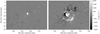 |
Fig. 1. Excerpts from the time series of reprojected magnetogram cut-outs produced with ELECTRICIT for AR 12673, showing the observed Bz component on 1 September 21:24 UT (left), and on 6 September 11:48 UT (right) just before the X9.3 flare. |
The time series of processed magnetograms from above is used to optimise the free parameters of the electric field inversion as described in Sect. 2.2, Lumme et al. (2017), and Pomoell et al. (2019). However, when deriving the photospheric boundary condition for the data-driven simulations, we process the magnetogram data even further to acquire better numerical stability and to save computational resources (see Pomoell et al. 2019 for details). This includes the temporal and spatial smoothing of the magnetograms, and rebinning them to four times lower spatial resolution. We further force the magnetic field to go smoothly to zero at the 20 outermost pixels, and then correct the flux imbalance of the magnetograms so that ∫ dABz = 0. This magnetogram series is used as the final input data for the electric field inversion (Sect. 2.2) and the data-driven simulation.
Finally, we should point out that the HMI magnetogram data had daily data gaps of ∼2 h throughout our analysis interval. The cut-out creation procedure within the ELECTRICIT toolkit automatically conformed to the data gaps when creating the original full resolution series, and we did not fill the data gaps in that series. However, for the rebinned and smoothed magnetogram series used as the final simulation input we filled the data gaps with linearly interpolated magnetograms before the temporal smoothing step. This ensured that the final electric field time series used in the simulation was temporally smooth around the data gaps.
2.2. Electric field inversion
The electric field inversion with ELECTRICIT (Lumme et al. 2017) is based on the decomposition of the electric field into the inductive EI and non-inductive −∇ψ components:
 (1)
(1)
The inductive component is fully constrained by Faraday’s law ∂tB = − ∇ × EI, and we solve it using the poloidal-toroidal decomposition (see Kazachenko et al. 2014 and Lumme et al. 2017 for details). Determining the non-inductive component would require photospheric velocity estimates (Schuck 2008; Kazachenko et al. 2014). However, due to the challenges of acquiring accurate photospheric plasma velocity estimates (Welsch et al. 2007, 2013), we instead approximate the non-inductive component using one of three previously employed ad hoc assumptions (Cheung & DeRosa 2012; Cheung et al. 2015; Lumme et al. 2017; Pomoell et al. 2019). First, the zeroth assumption simply sets the non-inductive component to zero. While it is known to be a poor assumption (Fisher et al. 2010; Cheung & DeRosa 2012), we retain it because it is an interesting point of comparison and because it is commonly used in other works (e.g. Yardley et al. 2018). Our second assumption is the U assumption of Cheung et al. (2015), in which the non-inductive potential ψ is solved via
 (2)
(2)
where U is a free parameter with units of velocity, and in very idealised settings (Cheung et al. 2015) it corresponds to the vertical emergence velocity of a twisted magnetic flux tube through the photosphere. The third and final assumption is the Omega assumption of Cheung & DeRosa (2012) for which
 (3)
(3)
where the Ω parameter has the units of rad s−1, and in highly idealised conditions corresponds to uniform vertical vorticity (∇ × V)z = −Ω related to the rotation of a vertical axisymmetric flux tube.
We chose the values of the free parameters Ω and U so that the respective electric field outputs optimally reproduce the total photospheric energy injection of a reference estimate calculated using the Differential Affine Velocity Estimator for Vector Magnetograms (DAVE4VM; see Lumme et al. 2017 for details). We computed the energy injection Em(t) by integrating, over time and area, the vertical Poynting flux as follows:
 (4)
(4)
We varied the free parameters Ω and U, estimated the energy injections for each value using Eq. (4), and chose the optimal values such that the root-mean-square difference between the reference DAVE4VM estimate and the Ω and U assumptions was minimised over the analysis interval. As an input to the optimisation we use the full-resolution reprojected magnetogram series discussed in Sect. 2.1, so that the daily data gaps in the series are included. The electric field inversion and DAVE4VM procedures conform to the data gaps such that the time derivatives of the magnetic field ∂B/∂t are estimated using the average change over the data gap.
After optimising the Ω and U parameters using the full-resolution magnetogram series, we switched to using the rebinned and smoothed magnetogram series, optimally designed to be used in driving the magnetofrictional simulation (see Sect. 2.1). We re-inverted the electric field using this data series and each of the three ad hoc assumptions above, with the Ω and U values optimised above. Unlike in Lumme et al. (2017) and Pomoell et al. (2019) we did not crop the whole 55-pixel zero-padding region temporarily added to each side of the magnetograms for the inversion (see Kazachenko et al. 2014 for details); instead, we retained 25 pixels of padding, as this helps to avoid significant dynamics at the boundaries of the data-driven simulation. These electric field series and the smoothed magnetogram data series were used as the final data-driven input to the magnetofrictional simulation.
2.3. Magnetofrictional modelling
We carried out simulations using the time-dependent data-driven magnetofrictional simulation described in Pomoell et al. (2019). The inverted horizontal photospheric electric fields are fed into the simulation as the data-driven lower boundary condition, and the first magnetogram (1 September 21:24 UT) was used to initialise the simulation using a potential field extrapolation. The response of the corona to the imposed evolution in the photosphere was computed by employing Faraday’s law with the electric field specified using a resistive MHD Ohm’s law in the coronal domain of the following form:
 (5)
(5)
The resistivity η was included in order to facilitate the change of topology of the magnetic field and was held uniform and constant at 200 × 106 m2 s−1. The magnetofrictional velocity field was computed as
 (6)
(6)
where ν is the frictional coefficient controlling the rate at which the coronal field relaxes, held constant at 1 × 10⁻¹¹ s m−2 except close to the lower boundary where 1/ν smoothly approaches zero as z → 0. This velocity is chosen such that the system evolves towards the minimum energy state where J × B = 0 and can be thought of as an approximation of the MHD momentum equation in a low-beta regime. This allows for the gradual buildup of magnetic energy and currents, such that the simulation is truly time-dependent instead of consisting of a series of extrapolations.
Simulations were carried out from 1 September 2017 21:24 UT, several days prior to the strong emergence, until 8 September 2017, at which time it was approaching the solar limb, which caused the HMI data to degrade due to the diminishing line-of-sight component. The simulation domain was chosen to have a height of 200 Mm in an attempt to ensure that the evolution of any eruptions would also be captured higher in the corona. The boundary conditions at the top and lateral sides were chosen to be open, allowing for magnetic flux to exit the domain (see Pomoell et al. 2019).
To assist with our analysis of the simulated output we used the method described in Liu et al. (2016) to calculate the squashing factor Q, which quantifies the divergence of nearby field lines and illustrates the locations of quasi-separatrix layers (QSLs) as regions with a high degree of squashing, and the twist number Tw which measures the turns of two infinitesimally close magnetic field lines about each other.
3. Results and discussion
Figure 2 shows the energy injection as computed using Eq. (4) for all three assumptions and for DAVE4VM (i.e. our reference estimate). The free parameters of the ad hoc assumptions were optimised as explained in Sect. 2.2 (values also shown in Fig. 2 legend). The time of the X9.3 flare is indicated by a dashed vertical line. Initially from 2 September 00:00 UT, until approximately 3 September 12:00 UT, the curves depicting the energy injection for each inversion appear to be in approximate agreement. However, after the start of the emergence around 4 September, the zeroth assumption (blue curve) begins to fall away from the reference value (red curve). After the X9.3 flare, the energy injection in the zero assumption levels off, while in the U and Ω assumptions and DAVE4VM it continues to increase. Following the flare, both the U and the Ω assumptions continue to agree with the reference estimate throughout most of the remaining time. However, the U assumption does begin to increasingly underestimate the energy approximately half a day after the X9.3 flare.
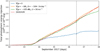 |
Fig. 2. Temporal evolution of the total photospheric energy injection for AR 12673 using the full-resolution magnetogram series, for the zeroth assumption (blue), the Ω assumption (orange), the U assumption (green), and the DAVE4VM reference value (red). The dashed vertical line indicates the time of the X9.3 flare. |
While the free parameters were optimised using the total photospheric energy injection, the total relative helicity injection was also studied as an additional metric due to its significance with regards to solar eruptions (e.g. Démoulin 2007; Pariat et al. 2017; Pomoell et al. 2019). We calculated this quantity as
 (7)
(7)
Figure 3 shows the total photospheric relative helicity injection for all three assumptions, and for the reference DAVE4VM electric fields, computed using Eq. (7). While initially in agreement with each other, the curves begin to significantly diverge late on 3 September, again after the start of the strong emergence but approximately twelve hours earlier than for the energy injection. The helicity injection in the zeroth assumption (blue curve) has only slight fluctuations, but otherwise remains just below zero throughout the time series. The U assumption (green curve) follows the trend of the reference value (red curve), but increasingly underestimates it, resulting in a factor of ∼2 difference at the end of the time series. The Ω assumption (orange curve), on the other hand, remains in close agreement with the reference value until early on 5 September, and then proceeds to increasingly overestimate the injected helicity. Previous studies conducted with ELECTRICIT, such as Lumme et al. (2017) and Pomoell et al. (2019), however, have shown considerably greater overestimation of the helicity by the Ω assumption. In Lumme et al. (2017), the Ω assumption began to overestimate the helicity over a day before the other cases started to increase from their initial values, and went on to be an order of magnitude greater by the end of the time series. The paper suggests that this behaviour likely arose because the non-inductive electric field component of the Ω assumption injects helicity with the same sign as Ω consistently over all pixels. The energy-optimised U assumption in turn underestimates the helicity injection similarly to Lumme et al. (2017) and Pomoell et al. (2019). One notable difference between the works is that unlike the ARs in the previous studies AR 12673 violates the hemispheric rule, which states that magnetic twist in ARs has a negative sign in the northern hemisphere and vice versa, shown to be accurate approximately 75% of the time (Liu et al. 2014). However, a much greater number of active regions need to be studied to definitively explain this difference in the performance of the Ω assumption.
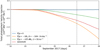 |
Fig. 3. Temporal evolution of the total photospheric helicity injection for AR 12673 for the zeroth assumption (blue), the Ω assumption (orange), the U assumption (green), and the DAVE4VM reference value (red). The horizontal dashed line indicates zero, while the dashed vertical line indicates the time of the X9.3 flare. |
3.1. Magnetic energy and helicity
To study the coronal response to the photospheric electric field, we used the electric field generated by the Ω assumption as input to the MFM simulation. This is because, as shown in Sect. 3, the Ω assumption provided the best correspondence with the DAVE4VM reference estimates for both photospheric energy and relative helicity injection.
We calculated both the total magnetic energy εM and the free magnetic energy εfree contained in the coronal domain as
 (8)
(8)
 (9)
(9)
where B denotes the magnetic field, Bp the potential field, and μ0 the permeability of free space or the magnetic constant. The top panel of Fig. 4 shows the total magnetic energy (purple curve) and free magnetic energy (blue curve), while the bottom panel shows the ratio of the free energy to the total magnetic energy. As shown in Fig. 4 the total coronal energy increases monotonically over time following the start of the emergence of the first bipoles at approximately 08:00 UT on 3 September. At this time, the ratio of the free energy to the total magnetic energy (εfree/εM) decreases from approximately 0.12 to 0.05. The subsequent rise in the ratio is likely related to the emergence of a further two bipoles. The ratio increases quickly, to approximately 0.20, until early on 5 September and then the rate of increase falls as the sunspot evolution becomes less drastic. The maximum value reached is 0.26. At approximately 09:00 UT on 6 September (i.e. at the time of the X2.2 flare), the total magnetic energy levels off for approximately three hours while the free magnetic energy continues to rise. This is consistent with the findings of Liu et al. (2018) who found using a time series of NLFFF extrapolations that the X2.2 flare increases the axial flux and helicity in the coronal flux rope structure, which could be expected to result in an increase in the free magnetic energy budget without a significant change in the total energy. Following this, and after the X9.3 class flare at 11:53 UT, the free magnetic energy levels off for the remainder of the day, while the total magnetic energy resumes rising. This is featured in the bottom panels of Fig. 4 as a decrease in the εfree/εM ratio (from approximately 0.26 to 0.21). After this, both the total and free magnetic energy, as well as the εfree/εM ratio, increase rather monotonically for the rest of the simulation. In a basic scenario, the free energy increase slowing down at the time of the eruption is consistent with the fact that the eruption is powered by the free energy (see e.g. Wiegelmann & Sakurai 2012, for discussion), and thus it would be expected that the eruption converts part of the free energy into kinetic energy. We note that the free energy remains below one-third of the total energy throughout the simulation time window. Additionally, we caution that the total magnetic energy in the simulation (Fig. 4) cannot be directly compared to the total energy injection derived from the photospheric electrograms and magnetograms (Fig. 2) because of the additional processing we do to the magnetograms (including smoothing and rebinning, see Sect. 2.1) that changes the injection, and because the horizontal magnetic field components in the lowest simulation cells are not forced to evolve as they do in the magnetograms (see Pomoell et al. 2019, for details).
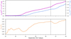 |
Fig. 4. Temporal evolution of magnetic energy. Top panel: total magnetic energy (purple) compared to the free magnetic energy (blue) on different scales. Bottom panel: ratio of the free magnetic energy to the total magnetic energy (orange). The dashed vertical line in each panel indicates the time of the X9.3 flare. |
The differences between the observed and the simulated horizontal magnetic fields are shown in Fig. 5. There are numerous methods for evaluating such differences in a time series of 2D maps, and here we select three of them. Following the example of Kazachenko et al. (2014), we use the slope of a least-squares polynomial fit and the linear Pearson correlation coefficient for the x and y magnetic field components separately (in an ideal case these metrics would be exactly 1). Additionally, we consider the angle between the observed input and the simulated output horizontal fields. We applied the same mask of 250 G used in the processing of the input magnetograms for the solid lines, and a mask of 1000 G for the dashed lines. The much higher masking serves to illustrate how certain differences are caused by the weak field regions. As our horizontal field is not forced to evolve as observed, the evident divergence between the input and output fields is expected. The slope suggests an overall fair agreement between the fields without revealing much regarding the simulation itself. However, the Pearson coefficient, which measures how well the quantities follow a linear relationship, indicates that initially the fields correlate very well but then increasingly differ over time, with a notable decrease in the Bx component just before the X9.3 flare. The mean angle follows the same behaviour as the Pearson correlation coefficient with an initial close agreement that increasingly diverges, though it appears to be unaffected by the major flare. The initial spiking behaviour in the mean angle is shown to be mostly confined to the weak field regions.
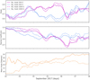 |
Fig. 5. Temporal evolution of metrics comparing the horizontal magnetic field of the observed input magnetograms vs. the simulated output magnetograms. Top and middle panels: slope and Pearson coefficient respectively, for Bx (purple) and By (blue). Bottom panel: mean angle between the input and output fields (orange). The solid lines use a mask of 250 G, while the dashed lines use a mask of 1000 G on the magnitude of the magnetic field vector. |
We additionally calculate the relative magnetic helicity for our simulation domain and decompose it, as in Berger. (2003), into the helicity of the current-carrying field and the mutual helicity between the current-carrying and the potential field as
 (10)
(10)
 (11)
(11)
 (12)
(12)
where HR denotes the relative magnetic helicity, A the vector potential of the magnetic field B, Ap the vector potential of the potential magnetic field Bp, Hj the helicity of the current-carrying field, and Hpj the mutual helicity between the current-carrying and the potential field. The top panel of Fig. 6 shows an increasing amount of absolute relative helicity and a steepening gradient over time, consistent with the photospheric injection estimates in Fig. 3. However, similarly to the energy injection, Fig. 6 is not directly comparable to the photospheric injection in Fig. 3 due to the additional processing we perform on the photospheric data before the simulation. Relative helicity continues to monotonically increase in magnitude throughout the simulation similar to the magnetic energy (Fig. 4) showing no prominent features related to the main phases of evolution of the AR (e.g. emergence of the bipoles, flares). The current-carrying helicity follows an almost identical trend, but with a noticeable decrease in magnitude following the X9.3 flare. The initial trend, however, is notably recovered following this decrease.
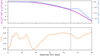 |
Fig. 6. Temporal evolution of helicity. Top panel: relative helicity (purple) compared to the helicity of the current-carrying magnetic field (blue) on different scales. Bottom panel: ratio of the current-carrying helicity to the relative helicity (orange). The dashed vertical line in each panel indicates the time of the X9.3 flare. |
The ratio of the current-carrying helicity to the relative helicity in the bottom panel of Fig. 6 reveals a clear trend however. The behaviour almost identically follows that of the free magnetic energy to the total magnetic energy, but with some scaling differences. However, we note that the current-carrying helicity appears to have a threshold of approximately 17% of the relative helicity, which is never exceeded. Zuccarello et al. (2018) presented evidence for such a threshold in simulations of torus unstable flux ropes, finding a ratio of approximately 0.29 ± 0.01. However, they noted that their number is unlikely to be universal because the relative helicity is not a simply additive quantity. While the large number of eruptions in this AR makes the situation more complicated, it is clear that there is a value that the ratio does not exceed. This serves to highlight the importance of helicity, and specifically this ratio, in studies of eruptions and their forecasting. However, we suggest that this ratio should not be considered in isolation, but in combination with free magnetic energy. The lower panel of Fig. 6 also shows that the ratio approached, but did not exceed, the threshold prior to 4 September even though there were no flares. During this time, the AR was principally a unipolar sunspot surrounded by some weak field regions until the large emergence began at 08:00 UT on 3 September. Accordingly, the free magnetic energy remained at its baseline as shown in the upper panel of Fig. 4.
3.2. Normalised Lorentz force and twist
To investigate the degree to which the magnetic field remains force-free during the evolution, we compute CWsin, the current-weighted sine between the current and the magnetic field (Metcalf et al. 2008) given by
 (13)
(13)
where
 (14)
(14)
A force-free field would have a CWsin of 0, while a non-force-free field would have a value of up to 1. The top panel of Fig. 7 shows the time-evolution of this metric for our simulation. While not shown, the metric begins at 0 due to our use of a potential field as the initial condition for the simulation. It quickly increases to approximately 0.3 because immediately after the electric field is applied, small currents are generated at the lower boundary which the magnetofriction relaxes more slowly due to the tapering of the velocity (see Sect. 2.5 and Eq. (4) of Pomoell et al. 2019). For the subsequent evolution, the metric remains between approximately 0.15 and 0.25, the same range as typically found when performing static NLFFF extrapolations (e.g. DeRosa et al. 2015). The metric shows a decreasing trend for approximately 2.5 days prior to the time of the X9.3 flare. However, at the time of the flare, a clear change in the trend occurs with a temporary increase in the Lorentz force taking place, indicating the destabilisation of the flux rope structure.
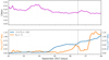 |
Fig. 7. Temporal evolution of metrics indicating the extent to which the magnetic field is force-free. Top panel: current-weighted sine between the current and the magnetic field (CWsin, purple). Bottom panel: magnetic flux with Tw < −1 (orange), and with −1 < Tw < −1/2 (blue). The curves are plotted on different scales. The dashed vertical line in each panel indicates the time of the X9.3 flare. |
In order to quantify the evolution and creation of magnetic structures in the simulation that contain twist, we group field lines in two categories: structures with moderate twist defined as having a twist value −1 < Tw < −1/2, and structures with high twist for which Tw < −1. The unsigned magnetic flux through the z = 0 plane of these structures is then determined. In the lower panel of Fig. 7 the result of this computation is shown. The figure shows a general increase in moderately twisted field throughout the simulation time, and that the unsigned magnetic flux of the moderately twisted structures is an order of magnitude higher than that of the highly twisted structures. During the first three days of the simulation, the flux carried by twisted structures increases only modestly followed by a rapid increase in the number of moderately twisted structures at approximately noon on 4 September. This rise is followed one day later by an increase in the flux carried by highly twisted structures, indicating the time of the formation of the large-scale flux rope in the simulation. At approximately 09:00 UT on 6 September there is a small but noticeable decrease in moderately twisted field at the same time as the highly twisted field peaks prior to the X9.3 flare. The subsequent decrease in highly twisted field before it rapidly increases, at approximately 5:00 UT on 7 September, is due to the reconnection taking place during this time.
3.3. Formation and evolution of erupting flux rope
Our magnetofrictional simulation illustrated the dynamic nature of the AR. By looking at the magnetic field lines, the current density, and other metrics such as the free magnetic energy and current-carrying helicity, there was evidence of clear activity throughout the simulation time. However, in this work we focus on the most prominent events during the simulation time, the two X-class flares, and the associated CME, on 6 September.
Figure 8 illustrates the key field lines in the simulation at the time of the X9.3 flare, a negatively twisted flux rope from A+ to A−, and a negatively twisted overlying neighbouring arcade-like system from B+ to B−. As shown by the inset, both of these structures share a common footpoint region bounded by a QSL and a twist of slightly less than −1. However, they go on to connect to two different negative polarity regions which are separated by a null point. As the simulation time progresses (see Fig. 9), flux from structure B reconnects via the null point to structure A, whose twist becomes visually increasingly apparent. This reconnection forms a single larger flux rope, clearly visible as a region of increased current density, that rises as the time progresses. Consequently, we associated this flux rope with the eruption producing the X9.3 flare. The null point persists following the eruption as shown by the white-purple field lines. Comparing the panels of Fig. 9 with the volume plots of magnetic energy and helicity (Figs. 4 and 6) we find all quantities to be steadily increasing in magnitude for the first panel (6 September 00:24 UT). The time of the second panel (6 September 12:24 UT) coincides with the beginning of the plateau in free magnetic energy, the decrease in absolute current-carrying helicity, and the noticeable trough in both magnetic energy and helicity ratios. The third panel (7 September 00:24 UT) coincides approximately with the middle of this trough, where the free magnetic energy and current-carrying helicity resumed rising approximately five hours earlier. The final panel (7 September 12:24 UT) is associated with the free magnetic energy and the current-carrying helicity almost having recovered their trends prior to the deviations.
The flux rope does not fully eject from our simulation domain; however, we postulate that this may be due to the nature of the magnetofrictional method. This is similar to the study of AR 11437 by Yardley et al. (2018) whose magnetofrictional simulation captured an erupting flux rope. They found their flux rope did not leave the simulation domain even when open top boundary conditions were applied. In our case, the helicity threshold was reached and the eruption was initiated, indicated by the rising structure, but the magnetofrictional relaxation caused it to find a new quasi-equilibrium before it could escape the domain. The footpoints of our flux rope are visually consistent with the footpoints of the eruptive magnetic flux rope found by Inoue et al. (2018) in their magnetohydrodynamic simulation of the X9.3 flare. Notably, the simulation of Inoue et al. (2018) was initialised with an NLFFF reconstruction 20 min prior to the X2.2 flare on 6 September, whereas our simulation was fully data-driven with inverted photospheric electric fields as the boundary condition from 1 September 21:24 UT. Consistency between our results and those of Inoue et al. (2018) imply that the two modelling approaches are similarly capable of reproducing the large-scale shape of the erupting flux rope structure, despite the large differences in the modelling schemes both in the plasma model (magnetofrictional versus MHD) and the temporal range.
To further investigate the performance of the simulation we compared the simulated magnetic field to EUV observations from AIA. Shown in the left panel of Fig. 10 is the AIA 94 Å observation from 6 September 08:58 UT corresponding to our simulation domain, while in the right panel is a corresponding Q map from 6 September 09:24 UT. Both panels have field lines consistent with Fig. 8 from 6 September 09:24 UT. Immediately apparent is the correspondence of the null point where the reconnection takes place in the simulations with the cusp-shaped brightening in the observations. However, this may also be the result of projection effects as the AR was already approximately 45° from disc centre at this time. The bright inverse U-shaped emission beneath the purple lines of the null point may instead be the cusp. Very similar footpoint locations have been found by Zou et al. (2019) in their NLFFF extrapolation just before the X2.2 flare on 6 September 08:36 UT, but the connectivity is different. The white-blue lines in Fig. 10 above the null point are shown to be in close proximity to a region of brightening, a direct signature of the yellow-blue lines reconnecting across with the white-purple field lines. The triangular cusp-like brightening between the footpoint of the yellow-blue field lines and the null point may correspond to a similar triangular shape in the Q map in the right panel, lending support to the actual cusp structure being the bright curve partially obscured by field lines in the vicinity of the null point.
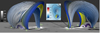 |
Fig. 8. Two snapshots from 6 September 12:24 UT from different viewing angles where the photosphere is represented by the simulated Bz magnetogram (white to black) with a colour bar in Tesla. Plotted are three sets of field lines: the white to blue lines which connect from A+ to A−, the yellow to blue lines which connect from B+ to B−, and the white to purple lines illustrating a null point between A− and B−. Also shown in the inset is an excerpt of a photospheric map of the twist Tw, with a colour bar from negative (blue) to positive (red), illustrating the seed points of the field lines from A+ and B+. A grey to black line is superposed onto the twist map illustrating the base 10 logarithmic squashing factor Q from 3 to 4. The structures reach a peak height of approximately 82 Mm. |
 |
Fig. 9. Simulation excerpts from 6 September 00:24 to 7 September 12:24 UT with a spacing of 12 h between each image. In the top row the flux rope associated with the X9.3 flare is bisected by a plane of the current density (pink to green), while the bottom row has this removed to provide an unobstructed view. The field lines are coloured as in Fig. 8, serving only to distinguish the bundles of lines and the different lines within each bundle. The flux rope reaches a peak height of approximately 150 Mm. |
 |
Fig. 10. Comparing an observation with the AIA 94 Å filter (left) and a photospheric map of the squashing factor Q from our simulations (right). The Q map is from 06 September 09:24 UT, while the time of the AIA observation was 06 September 08:59 UT because the observations were saturated closer to 09:24 UT due to the onset of the X2.2 flare at 08:57 UT. Also shown are the key field lines, consistent with Fig. 8 with minor footpoint adjustments due to time. The field lines are from 06 September 09:24 in both panels. |
4. Conclusions
We conducted fully data-driven time-dependent magnetofrictional modelling of AR 12673, from 1 September 21:24 UT until 8 September, using an electric field inverted from HMI vector magnetograms. The simulation captured the most prominent feature of the active region, the X9.3 flare and its accompanying CME flux rope eruption, and showed indications of other eruptive features such as curved structures of enhanced current density ejecting from the domain. We found that there was reconnection between the flux rope and a nearby sheared arcade, which overlies part of the flux rope, mediated by a nearby null point. The analysis was additionally aided by computing maps of the squashing factor and twist, and by comparison to EUV observations. Consequently, it was found that the simulated structure is consistent with observed EUV brightenings.
In this paper, we demonstrated a possible threshold for eruptions in the ratio of current-carrying helicity to relative helicity (Fig. 6) using a data-driven simulation, supporting the findings of Pariat et al. (2017) and Zuccarello et al. (2018) whose idealised simulations suggested that such a threshold exists. While we do not believe that reaching the threshold is always required for an eruption to take place, we suggest that an eruption becomes increasingly likely as the ratio approaches it. Further case studies are certainly needed to evaluate this relationship as rigorously as possible, and to explore its potential use in forecasting solar eruptions and space weather. The ratio of the free magnetic energy to the total magnetic energy in our study (Fig. 4) evolves similarly to the ratio in helicity, such that they both provide a clear indication of the time of the X9.3 flare, except that it generally increases over time instead of suggesting a threshold. However, we suggest that the helicity ratio should be considered in combination with the free magnetic energy. As shown by the lower panel of Fig. 6, the threshold appeared to be respected even before the AR had fully emerged. During this time there were no eruptions, but this is understandable as the free magnetic energy is still at its baseline (Fig. 4). We cannot say for certain whether the behaviour of the helicity ratio was governed by the threshold during the early evolution of the AR, which would suggest an underlying physical mechanism responsible, or if it was merely a coincidence. However, further studies of more ARs are clearly warranted.
Additionally we showed that the fully data-driven magnetofrictional method is able to generate eruptive solar structures consistent with EUV observations, and generate structures with footpoints consistent with other methods which are only data-constrained. The time-dependent nature of our simulations allowed us to explain the evolution of the magnetic field and demonstrate the reconnection which lead to the eruption of the flux rope associated with the X9.3 flare. We note that while our flux rope did not eject from the simulation domain, we used the word eruption because the initiation of the eruption was captured as evidenced by the reconnecting and rising flux rope structure. We suggest that the rising was slowed and the flux rope prevented from leaving the domain due to the nature of the magnetofrictional method in the sense that it is continually trying to relax the field to a force-free state. Rectifying this, potentially by finding a way to make the simulated field more unstable during eruptions, could be a focus of future work.
Acknowledgments
This project has received funding from the European Research Council (ERC) under the European Union’s Horizon 2020 research and innovation programme (grant agreement No 724391). The work leading to these results has been carried out in the Finnish Centre of Excellence in Research of Sustainable Space (Academy of Finland grant number 312390). SDO data are courtesy of NASA/SDO and the AIA and HMI science teams. This research has made use of NASA’s Astrophysics Data System. EL acknowledges the Doctoral Programme in Particle Physics and Universe Sciences (PAPU) of the University of Helsinki for financial support. EK and DP acknowledge the Finnish Society of Sciences and Letters and the Ruth och Nils-Erik Stenbäcks stipendium.
References
- Berdermann, J., Kriegel, M., Banyś, D., et al. 2018, Space Weather, 16, 1604 [NASA ADS] [CrossRef] [Google Scholar]
- Berger, M. A. 2003, in Topological Quantities in Magnetohydrodynamics, eds. A. Ferriz-Mas, & M. Núñez, 345 [Google Scholar]
- Chen, J. 2017, Phys. Plasmas, 24, 090501 [NASA ADS] [CrossRef] [Google Scholar]
- Chertok, I. M., Belov, A. V., & Abunin, A. A. 2018, Space Weather, 16, 1549 [NASA ADS] [CrossRef] [Google Scholar]
- Cheung, M. C. M., & DeRosa, M. L. 2012, ApJ, 757, 147 [NASA ADS] [CrossRef] [Google Scholar]
- Cheung, M. C. M., De Pontieu, B., Tarbell, T. D., et al. 2015, ApJ, 801, 83 [NASA ADS] [CrossRef] [Google Scholar]
- Démoulin, P. 2007, Adv. Space Rev., 39, 1674 [Google Scholar]
- DeRosa, M. L., Wheatland, M. S., Leka, K. D., et al. 2015, ApJ, 811, 107 [NASA ADS] [CrossRef] [Google Scholar]
- Eastwood, J. P., Hapgood, M. A., Biffis, E., et al. 2018, Space Weather, 16, 2052 [NASA ADS] [CrossRef] [Google Scholar]
- Fisher, G. H., Welsch, B. T., Abbett, W. P., & Bercik, D. J. 2010, ApJ, 715, 242 [NASA ADS] [CrossRef] [Google Scholar]
- Fisher, G. H., Abbett, W. P., Bercik, D. J., et al. 2015, Space Weather, 13, 369 [NASA ADS] [CrossRef] [Google Scholar]
- Forbes, T. G. 2000, J. Geophys. Res., 105, 23153 [NASA ADS] [CrossRef] [Google Scholar]
- Green, L. M., Török, T., Vršnak, B., Manchester, W., & Veronig, A. 2018, Space Sci Rev., 214, 46 [NASA ADS] [CrossRef] [Google Scholar]
- Hayashi, K., Feng, X., Xiong, M., & Jiang, C. 2018, ApJ, 855, 11 [Google Scholar]
- Hayashi, K., Feng, X., Xiong, M., & Jiang, C. 2019, ApJ, 871, L28 [NASA ADS] [CrossRef] [Google Scholar]
- Hoeksema, J. T., Liu, Y., Hayashi, K., et al. 2014, Sol. Phys., 289, 3483 [Google Scholar]
- Hou, Y. J., Zhang, J., Li, T., Yang, S. H., & Li, X. H. 2018, A&A, 619, A100 [NASA ADS] [CrossRef] [EDP Sciences] [Google Scholar]
- Inoue, S. 2016, Progr. Earth Planet. Sci., 3, 19 [NASA ADS] [CrossRef] [Google Scholar]
- Inoue, S., Shiota, D., Bamba, Y., & Park, S.-H. 2018, ApJ, 867, 83 [NASA ADS] [CrossRef] [Google Scholar]
- James, A. W., Green, L. M., Palmerio, E., et al. 2017, Sol. Phys., 292, 71 [NASA ADS] [CrossRef] [Google Scholar]
- Jiang, C., Wu, S. T., Feng, X., & Hu, Q. 2016a, Nat. Commun., 7, 11522 [Google Scholar]
- Jiang, C., Wu, S. T., Yurchyshyn, V., et al. 2016b, ApJ, 828, 62 [NASA ADS] [CrossRef] [Google Scholar]
- Jiang, C., Zou, P., Feng, X., et al. 2018, ApJ, 869, 13 [NASA ADS] [CrossRef] [Google Scholar]
- Kazachenko, M. D., Fisher, G. H., & Welsch, B. T. 2014, ApJ, 795, 17 [Google Scholar]
- Kazachenko, M. D., Fisher, G. H., Welsch, B. T., Liu, Y., & Sun, X. 2015, ApJ, 811, 16 [NASA ADS] [CrossRef] [Google Scholar]
- Kilpua, E., Lugaz, N., Mays, L., & Temmer, M. 2019, Space Weather, 17, 498 [NASA ADS] [CrossRef] [Google Scholar]
- Kliem, B., & Török, T. 2006, Phys. Rev. Lett., 96, 255002 [NASA ADS] [CrossRef] [PubMed] [Google Scholar]
- Lemen, J. R., Title, A. M., Akin, D. J., et al. 2012, Sol. Phys., 275, 17 [NASA ADS] [CrossRef] [Google Scholar]
- Liu, Y., Hoeksema, J. T., & Sun, X. 2014, ApJ, 783, L1 [NASA ADS] [CrossRef] [Google Scholar]
- Liu, R., Kliem, B., Titov, V. S., et al. 2016, ApJ, 818, 148 [NASA ADS] [CrossRef] [Google Scholar]
- Liu, L., Cheng, X., Wang, Y., et al. 2018, ApJ, 867, L5 [NASA ADS] [CrossRef] [Google Scholar]
- Lumme, E., Pomoell, J., & Kilpua, E. K. J. 2017, Sol. Phys., 292, 191 [NASA ADS] [CrossRef] [Google Scholar]
- Metcalf, T. R., De Rosa, M. L., Schrijver, C. J., et al. 2008, Sol. Phys., 247, 269 [Google Scholar]
- Morosan, D. E., Carley, E. P., Hayes, L. A., et al. 2019, Nat. Astron., 3, 452 [NASA ADS] [CrossRef] [Google Scholar]
- Pariat, E., Leake, J. E., Valori, G., et al. 2017, A&A, 601, A125 [NASA ADS] [CrossRef] [EDP Sciences] [Google Scholar]
- Pesnell, W. D., Thompson, B. J., & Chamberlin, P. C. 2012, Sol. Phys., 275, 3 [NASA ADS] [CrossRef] [Google Scholar]
- Pomoell, J., Lumme, E., & Kilpua, E. 2019, Sol. Phys., 294, 41 [NASA ADS] [CrossRef] [Google Scholar]
- Qiu, J., Hu, Q., Howard, T. A., & Yurchyshyn, V. B. 2007, ApJ, 659, 758 [NASA ADS] [CrossRef] [Google Scholar]
- Redmon, R. J., Seaton, D. B., Steenburgh, R., He, J., & Rodriguez, J. V. 2018, Space Weather, 16, 1190 [NASA ADS] [CrossRef] [Google Scholar]
- Romano, P., Elmhamdi, A., & Kordi, A. S. 2019, Sol. Phys., 294, 4 [NASA ADS] [CrossRef] [Google Scholar]
- Scherrer, P. H., Schou, J., Bush, R. I., et al. 2012, Sol. Phys., 275, 207 [Google Scholar]
- Schillings, A., Nilsson, H., Slapak, R., et al. 2018, Space Weather, 16, 1363 [NASA ADS] [CrossRef] [Google Scholar]
- Schrijver, C. J., Kauristie, K., Aylward, A. D., et al. 2015, Adv. Space Rev., 55, 2745 [Google Scholar]
- Schuck, P. W. 2008, ApJ, 683, 1134 [NASA ADS] [CrossRef] [Google Scholar]
- Sun, X., & Norton, A. A. 2017, Res. Notes Am. Astron. Soc., 1, 24 [NASA ADS] [CrossRef] [Google Scholar]
- Temmer, M., Thalmann, J. K., Dissauer, K., et al. 2017, Sol. Phys., 292, 93 [Google Scholar]
- Török, T., Kliem, B., & Titov, V. S. 2004, A&A, 413, L27 [NASA ADS] [CrossRef] [EDP Sciences] [Google Scholar]
- van Ballegooijen, A. A., Priest, E. R., & Mackay, D. H. 2000, ApJ, 539, 983 [NASA ADS] [CrossRef] [Google Scholar]
- Verma, M. 2018, A&A, 612, A101 [NASA ADS] [CrossRef] [EDP Sciences] [Google Scholar]
- Vourlidas, A., Lynch, B. J., Howard, R. A., & Li, Y. 2013, Sol. Phys., 284, 179 [NASA ADS] [Google Scholar]
- Vourlidas, A., Balmaceda, L. A., Stenborg, G., & Dal Lago, A. 2017, ApJ, 838, 141 [NASA ADS] [CrossRef] [Google Scholar]
- Wang, W., Liu, R., Wang, Y., et al. 2017, Nat. Commun., 8, 1330 [NASA ADS] [CrossRef] [Google Scholar]
- Webb, D. F., & Howard, T. A. 2012, Liv. Rev. Sol. Phys., 9, 3 [Google Scholar]
- Welsch, B. T. 2018, Sol. Phys., 293, 113 [NASA ADS] [CrossRef] [Google Scholar]
- Welsch, B. T., Abbett, W. P., De Rosa, M. L., et al. 2007, ApJ, 670, 1434 [NASA ADS] [CrossRef] [Google Scholar]
- Welsch, B. T., Fisher, G. H., & Sun, X. 2013, ApJ, 765, 98 [NASA ADS] [CrossRef] [Google Scholar]
- Wiegelmann, T., & Sakurai, T. 2012, Liv. Rev. Sol. Phys., 9, 5 [Google Scholar]
- Wiegelmann, T., Petrie, G. J. D., & Riley, P. 2017, Space Sci. Rev., 210, 249 [NASA ADS] [CrossRef] [Google Scholar]
- Yan, X. L., Wang, J. C., Pan, G. M., et al. 2018, ApJ, 856, 79 [NASA ADS] [CrossRef] [Google Scholar]
- Yang, S., Zhang, J., Zhu, X., & Song, Q. 2017, ApJ, 849, L21 [NASA ADS] [CrossRef] [Google Scholar]
- Yang, W. H., Sturrock, P. A., & Antiochos, S. K. 1986, ApJ, 309, 383 [NASA ADS] [CrossRef] [Google Scholar]
- Yardley, S. L., Mackay, D. H., & Green, L. M. 2018, ApJ, 852, 82 [NASA ADS] [CrossRef] [Google Scholar]
- Yasyukevich, Y., Astafyeva, E., Padokhin, A., et al. 2018, Space Weather, 16, 1013 [NASA ADS] [CrossRef] [PubMed] [Google Scholar]
- Zou, P., Jiang, C., Feng, X., et al. 2019, ApJ, 870, 97 [NASA ADS] [CrossRef] [Google Scholar]
- Zuccarello, F. P., Pariat, E., Valori, G., & Linan, L. 2018, ApJ, 863, 41 [Google Scholar]
All Figures
|
Fig. 1. Excerpts from the time series of reprojected magnetogram cut-outs produced with ELECTRICIT for AR 12673, showing the observed Bz component on 1 September 21:24 UT (left), and on 6 September 11:48 UT (right) just before the X9.3 flare. |
| In the text | |
|
Fig. 2. Temporal evolution of the total photospheric energy injection for AR 12673 using the full-resolution magnetogram series, for the zeroth assumption (blue), the Ω assumption (orange), the U assumption (green), and the DAVE4VM reference value (red). The dashed vertical line indicates the time of the X9.3 flare. |
| In the text | |
|
Fig. 3. Temporal evolution of the total photospheric helicity injection for AR 12673 for the zeroth assumption (blue), the Ω assumption (orange), the U assumption (green), and the DAVE4VM reference value (red). The horizontal dashed line indicates zero, while the dashed vertical line indicates the time of the X9.3 flare. |
| In the text | |
|
Fig. 4. Temporal evolution of magnetic energy. Top panel: total magnetic energy (purple) compared to the free magnetic energy (blue) on different scales. Bottom panel: ratio of the free magnetic energy to the total magnetic energy (orange). The dashed vertical line in each panel indicates the time of the X9.3 flare. |
| In the text | |
|
Fig. 5. Temporal evolution of metrics comparing the horizontal magnetic field of the observed input magnetograms vs. the simulated output magnetograms. Top and middle panels: slope and Pearson coefficient respectively, for Bx (purple) and By (blue). Bottom panel: mean angle between the input and output fields (orange). The solid lines use a mask of 250 G, while the dashed lines use a mask of 1000 G on the magnitude of the magnetic field vector. |
| In the text | |
|
Fig. 6. Temporal evolution of helicity. Top panel: relative helicity (purple) compared to the helicity of the current-carrying magnetic field (blue) on different scales. Bottom panel: ratio of the current-carrying helicity to the relative helicity (orange). The dashed vertical line in each panel indicates the time of the X9.3 flare. |
| In the text | |
|
Fig. 7. Temporal evolution of metrics indicating the extent to which the magnetic field is force-free. Top panel: current-weighted sine between the current and the magnetic field (CWsin, purple). Bottom panel: magnetic flux with Tw < −1 (orange), and with −1 < Tw < −1/2 (blue). The curves are plotted on different scales. The dashed vertical line in each panel indicates the time of the X9.3 flare. |
| In the text | |
|
Fig. 8. Two snapshots from 6 September 12:24 UT from different viewing angles where the photosphere is represented by the simulated Bz magnetogram (white to black) with a colour bar in Tesla. Plotted are three sets of field lines: the white to blue lines which connect from A+ to A−, the yellow to blue lines which connect from B+ to B−, and the white to purple lines illustrating a null point between A− and B−. Also shown in the inset is an excerpt of a photospheric map of the twist Tw, with a colour bar from negative (blue) to positive (red), illustrating the seed points of the field lines from A+ and B+. A grey to black line is superposed onto the twist map illustrating the base 10 logarithmic squashing factor Q from 3 to 4. The structures reach a peak height of approximately 82 Mm. |
| In the text | |
|
Fig. 9. Simulation excerpts from 6 September 00:24 to 7 September 12:24 UT with a spacing of 12 h between each image. In the top row the flux rope associated with the X9.3 flare is bisected by a plane of the current density (pink to green), while the bottom row has this removed to provide an unobstructed view. The field lines are coloured as in Fig. 8, serving only to distinguish the bundles of lines and the different lines within each bundle. The flux rope reaches a peak height of approximately 150 Mm. |
| In the text | |
|
Fig. 10. Comparing an observation with the AIA 94 Å filter (left) and a photospheric map of the squashing factor Q from our simulations (right). The Q map is from 06 September 09:24 UT, while the time of the AIA observation was 06 September 08:59 UT because the observations were saturated closer to 09:24 UT due to the onset of the X2.2 flare at 08:57 UT. Also shown are the key field lines, consistent with Fig. 8 with minor footpoint adjustments due to time. The field lines are from 06 September 09:24 in both panels. |
| In the text | |
Current usage metrics show cumulative count of Article Views (full-text article views including HTML views, PDF and ePub downloads, according to the available data) and Abstracts Views on Vision4Press platform.
Data correspond to usage on the plateform after 2015. The current usage metrics is available 48-96 hours after online publication and is updated daily on week days.
Initial download of the metrics may take a while.