| Issue |
A&A
Volume 627, July 2019
|
|
|---|---|---|
| Article Number | A155 | |
| Number of page(s) | 16 | |
| Section | Planets and planetary systems | |
| DOI | https://doi.org/10.1051/0004-6361/201935773 | |
| Published online | 17 July 2019 | |
Global mapping of lunar refractory elements: multivariate regression vs. machine learning
1
Physical Research Laboratory,
Ahmedabad
380009, India
e-mail: megha@prl.res.in
2
Image Analysis Group, Dortmund University of Technology, Otto-Hahn Str. 4,
44227
Dortmund, Germany
e-mail: christian.woehler@tu-dortmund.de
3
School of Advanced Science and Engineering, Waseda University,
Tokyo
1698555, Japan
4
Research Institute for Science and Engineering, Waseda University,
Tokyo
1698555, Japan
5
National Institute for Quantum and Radiological Science and Technology (QST),
Chiba
2638555, Japan
Received:
25
April
2019
Accepted:
5
June
2019
Context. The quantitative estimation of elemental concentrations at the spatial resolution of hyperspectral near-infrared (NIR) images of the lunar surface is an important tool for understanding the processes relevant for the origin and evolution of the Moon.
Aims. We aim to map the abundances of the elements Fe, Ca, and Mg at a typical accuracy of about 1 wt.% at the spatial resolution of the Moon Mineralogy Mapper (M3) instrument on-board Chandrayaan-1 lunar mission.
Methods. The NIR reflectance of the lunar regolith is an integrated response to the presence of refractory elements and soil alteration processes. Our approach was to define a combination of spectral parameters that are robust with respect to the effects of soil maturity. We calibrated the spectral parameters with respect to elemental abundances measured by the Lunar Prospector Gamma Ray Spectrometer (LP GRS) and the Kaguya GRS (KGRS). For this purpose, we compared a classical multivariate linear regression (MLR) approach and the machine learning based support vector regression (SVR) technique applied to M3 global observations.
Results. The M3-based global elemental maps are consistent in distribution and range with the LP GRS and KGRS elemental maps and do not show artifacts in immature areas such as small fresh craters. The results derived using MLR and SVR are compared to sample-based ground truth data of the Apollo and Luna sample-return sites, where the root-mean-square deviations obtained by the two regression models are similar.
Conclusions. The main advantage of the proposed new algorithm is its ability to minimize artifacts due to space-weathering effects. The elemental maps of Mg and Ca provide additional information and reveal structures not always visible in the Fe map. The global elemental abundance maps derived for the fully calibrated M3 observations might thus serve as important tools to investigate the lunar geology and evolution.
Key words: methods: observational / Moon / planets and satellites: surfaces / techniques: spectroscopic / techniques: imaging spectroscopy / planets and satellites: composition
© ESO 2019
1 Introduction
The nearly global coverage of the surface of the Moon in the visible (VIS) to near-infrared (NIR) wavelength range using hyperspectral or multispectral imaging spectrometers can be used efficiently for estimating abundances of refractory elements such as Fe, Ti, Ca and Mg (Lucey et al. 1995; Shkuratov et al. 2005; Wöhler et al. 2011; Wu et al. 2012; Otake et al. 2012; Bhatt et al. 2012). The spatial resolution of elemental maps derived using the VIS-NIR spectroscopy is in the range of hundreds of meters in contrast to the at least two orders of magnitude lower spatial resolution of gamma-ray and X-ray spectrometers (tens of kilometers) (Lawrence et al. 1998, 2002; Crawford et al. 2009). The derived global maps of Fe and Ti using VIS-NIR multispectral data of the Clementine mission led to a better understanding of the origin and evolution processes of the Moon (Lucey et al. 1995; Le Mouélic et al. 2002; Kramer et al. 2008). The estimation of refractory elements in the VIS-NIR range either relies on empirical relationships between the derived spectral parameters and in situ chemical analyses of returned lunar samples (Lucey et al. 1995, 1998, 2000b; Blewett et al. 1997a; Le Mouélic et al. 2002; Bhatt et al. 2012, 2015) or on a global elemental estimation derived using remotely sensed gamma ray spectrometer (GRS) data as a reference (Shkuratov et al. 2005; Wöhler et al. 2011, 2014).
The spectral parameters band depth, band center, band width, and spectral continuum slope can be computed from the two pronounced absorption bands around 1 and 2 μm wavelengths (band I and band II hereafter). These absorption bands are a sensitive indicator of chemical composition due to the Fe2+ transition at the crystallographic sites of different minerals (Burns 1993). The combination of band I and band II spectral parameters provides information on the presence of the dominant mafic minerals; low-calcium pyroxene, high-calcium pyroxene, olivine, and ilmenite. The band depth and the slope of the spectral continuum are not only dependent on the mineral composition but also on surface maturity caused by space weathering effects (McKay et al. 1991; Keller & McKay 1993; Hapke 2001; Le Mouélic et al. 2002). Hence, the successful estimation of refectory elements in the VIS-NIR range depends on the choice of spectral parameters that can decouple maturity from lunar soil composition. Most of the elemental estimation algorithms derived from multispectral or hyperspectral data either use spectral parameters derived from absorption band I (Lucey et al. 1995, 1998, 2000b; Fischer & Pieters 1996; Blewett et al. 1997b,a; Le Mouélic et al. 2000; Lawrence et al. 2002; Gillis et al. 2004; Wöhler et al. 2011; Wu et al. 2012; Otake et al. 2012) or band II (Bhatt et al. 2012, 2015), but not both absorption bands.
Lucey et al. (1995, 1998, 2000b) developed iron estimation algorithms by defining an iron sensitive parameter derived from the relation of the ratio between the reflectances at 950 and 750 nm vs. the 750 nm reflectance (ratio-reflectance plot) using selected returned lunar samples, and applied them to the multispectral Clementine data. This iron estimation algorithm is based on the roughly orthogonal relationship in the ratio-reflectance plot of the spectral effects caused by the presence of Fe2+ in silicates and due to space-weathering effects. The iron estimation algorithm of Lucey et al. (2000b) provided an accuracy of about 1 wt.% when applied to lunar samples with a restricted range of iron contents and variable soil maturity. The coordinates of the reference point used for computing the FeO-sensitive angular parameter were inferred by Lucey et al. (2000b) from the ratio-reflectance plot by manual adjustment in order to minimize the maturity effects. This algorithm, though, showed strong dependencies on topography especially at high incidence angles when applied to the global multispectral Clementine UV/VIS dataset (Lucey et al. 1998, 2000a). Lucey’s approach was subsequently improved by Wilcox et al. (2005) in order to better compensate for maturity trends specifically in mare basalt regions. Le Mouélic et al. (2000) developed a new iron estimation algorithm by including the Clementine reflectance at 1500 nm to estimate the continuum slope across band I along with the reflectance at the Clementine 750 and 950 nm channels. This algorithm estimated the total FeO content as the sum of iron contained in both silicates and oxides by successfully minimizing the maturity effects (Lucey 2006). Bhatt et al. (2012, 2015) extended the approach of Le Mouélic et al. (2000) to the datasets of the instruments Infrared Spectrometer (SIR-2; Mall et al. 2009) and Moon Mineralogy Mapper (M3; Pieters et al. 2009) on-board Chandrayaan-1 and developed an iron estimation algorithm based on the band II spectral parameters. This approach successfully minimized maturity effects in mare regions, but the iron content of olivine-rich areas was underestimated. Another M3-based technique consists of the extraction of a set of spectral parameters inferred from both band I and band II of M3 spectra and developing a statistically-based regression model to estimate the abundances of Fe, Ti, Mg, and Ca, considering the elemental maps derived from Lunar Prospector Gamma Ray Spectrometer (LP GRS) measurements (Elphic et al. 1998) as a “ground truth” (Wöhler et al. 2014; Bhatt et al. 2015). This approach provides a consistent elemental abundance estimation on global scales but shows a dependency on maturity. In a recent study, Xia et al. (2019) developed a neural network model applied to data of the Interference Imaging Spectrometer instrument on-board Chang’E-1. This model was trained on the lunar sampling sites and was applied to Interference Imaging Spectrometer global coverage data to estimate the abundances of the oxides of Si, Al, Ca, Fe, Mg, Ti. The spectral range used in that work is from 522 to 918 nm. The algorithm directly relies on absolute reflectance values rather than spectral parameters sensitive to specific elemental abundances. A probable limitation of this direct machine learning based approach is that according to the maps shown by Xia et al. (2019) the main spectral property determining all estimated elemental abundances appears to be the surface albedo.
The objective of this study is to develop empirical multivariate regression models to estimate the abundances of the refractory elements Fe, Mg, and Ca on the Moon, by defining a set of spectral parameters that minimizes the sensitivity to maturity. For this purpose, the classical approach of multivariate linear regression (MLR) and the machine learning technique of support vector regression (SVR) are employed, where the input for both regression techniques is kept exactly the same. Our mapping approach relies on a thermally, topographically, and photometrically corrected M3 spectral reflectance mosaic of 20 pixels per degree resolution in the wavelength range between 0.67 and 2.6 μm. LP GRS and Kaguya GRS (KGRS) global elemental abundance maps have been considered as ground truth information for the regression. Different combinations of regression techniques and GRS data are validated on elemental abundance data of the Apollo and Luna sample return sites and are applied globally. The results derived using the new MLR and SVR models are compared to previous approaches with respect to the absolute level of the elemental abundances and the sensitivity to soil maturity.
2 Data and methods
We extracted band I and band II spectral parameters from a topographically and thermally corrected M3 global mosaic constructed using a previously published framework (Wöhler et al. 2014, 2017a,b; Grumpe et al. 2019). The level 1B M3 radiance dataset witha spatial resolution of 140 m/pixel (Pieters et al. 2009) has been resampled to a 20 pixels per degree (1.5 km/pixel at the equator)global mosaic. This reduction of the resolution leads to a reduction of the influence of the imperfect georeferencing of the M3 data and to an improvement of the signal-to-noise ratio by about an order of magnitude when compared to 140 m/pixel (full-resolution) M3 data. The topography correction was performed using the SLDEM512 topographic map (Barker et al. 2016). The topographic information is used for computing the solar incidence angle and emission angle for each pixel of each downsampled M3 image used. For each pixel of the global mosaic, based on all available radiance values typically acquired under different illumination conditions, a best-fit single-scattering albedo is computed based on the Hapke model (Hapke 1984, 2002). Eventually, the Hapke model is used to compute the spectral reflectances for all M3 channel wavelengths normalized to the uniform illumination and viewing geometry of 30° incidence angle and 0° emission angle (Pieters et al. 1994). At the reduced resolution of 20 pixels per degree, the quality of the georeferencing of the M3 data is usually good enough that the M3 can be used directly in combination with the SLDEM512. At full M3 resolution, however (Figs. 5 and 6), we performed a manual georeferencing of the M3 images with respectto the LROC WAC mosaic (Speyerer et al. 2011) and constructed high-resolution topographic maps of the regions under study using a shape from shading based method (Grumpe et al. 2014; Grumpe & Wöhler 2014). Further details about our topographic correction and normalization approach are given by Wöhler et al. (2014).The topographic data are also used for correction of the M3 level 1B spectral radiance data for the thermal emission of the surface. The accurate thermal emission removal is a very important step of the data processing because the presence of a thermal emission component may affect the band II spectral parameters, leading to possible misinterpretations of the mafic composition based on the wavelength range beyond 2 μm. The thermal correction applied to the M3 global mosaic is based on a physical model (Shkuratov et al. 2011) and iteratively adjusts spectral reflectance, spectral emissivity and surface temperature in a self-consistent manner (Wöhler et al. 2017a,b; Grumpe et al. 2019). The radiance has been converted to bidirectional reflectance at the uniform illumination and observation geometry of 30° incidence angle and 0° emission angle (Pieters 1999) using the reflectance model of Hapke (2002, 2012).
The band I and band II spectral parameters were extracted from the M3 smoothed reflectance spectra after removing the continuum using the convex hull of the spectrum (Fu et al. 2007). According to that approach, the wavelengths based on which the continuum slopes are computed are not fixed but given by the wavelengths at which the convex hull intersects the reflectance spectrum. We applied smoothening along the wavelength axis using a smoothing spline (Marsland 2015) for reducing the effect of channel noise. We selected a set of seven spectral parameters as follows:
- 1.
Band I and band II center wavelength (LMIN1 and LMIN2): determined as the location of the minimum of the continuum-removed reflectance value in the 1 and 2-μm absorption band, respectively;
- 2.
Band I and band II depth (BD1 and BD2): values of the continuum-removed reflectances at the center wavelengths, subtracted from 1;
- 3.
Full width at half maximum of band I (FWHM1): determined as the full width at half maximum of band I in the continuum-removed reflectance spectrum;
- 4.
Normalized continuum slopes at band I and band II (NCLS1 and NCLS2): determined as the continuum slopes across band I and band II, normalized to the reflectances at 0.75 and 1.57 μm, respectively.
Additionally, we used LP GRS global elemental maps of Fe, Ca and Mg and KGRS global maps of Fe and Ca at 0.2 pixels per degree spatial resolution as a reference. The LP GRS based global maps were constructed by Lawrence et al. (1998) and Prettyman et al. (2006) and have already been used as a reference by Shkuratov et al. (2005) and Wöhler et al. (2011, 2014) in their regression-based elemental estimation algorithms. The KGRS based global maps of Fe and Ca were constructed by Yamashita et al. (2012) and Naito et al. (2018) and were used here in a form spatially accumulated to 5° × 5° pixels. We down-sampled our M3 global mosaic to 0.2 pixels per degree spatial resolution and extracted a set of seven spectral parameters for the location of each LP GRS and KGRS pixel.
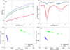 |
Fig. 1 Representative spectra of fresh crater locations from highland and mare regions and their respective band depth vs. continuum slope trends. The fresh crater locations from highland and mare region are marked as yellow squares in Fig. 2. (a) Reflectance spectra extracted from the interior to the outer rim of the ejecta blanket in sequence to demonstrate the decrease in band depth with increasing maturity. (b) Continuum-removed reflectance spectra of (a), clearly showing gradual changes in band depth as we move gradually away from a small crater. The representative spectra of highland in this case are offset by 0.03 for a clear representation. (c, d) Normalized continuum slope vs. band depth plots for band I and band II, respectively, showing linear trends for fresh crater locations from highland and mare regions. Maturity increases towards higher normalized continum slope and lower band depth values. The continuum slopes of band I and band II were normalized to the 0.75 and 1.57 μm reflectances,respectively. |
2.1 Regression-based elemental abundance using maturity independent spectral parameters
2.1.1 Identification of a set of maturity-independent spectral parameters
The most important part of the proposed elemental abundance estimation algorithm is the selection of maturity-independent spectral parameters. Maturity effects modify the spectral slope, band depth, and albedo in the NIR wavelength range, but the band center position remains unaffected (Pieters et al. 2000; Taylor et al. 2001). The reflectance spectra and corresponding continuum-removed spectra from typical mare and highland regions are shown in Figs. 1a and b. The set of spectra extracted from the locations marked with a square symbol in Fig. 2 are extracted in a sequence from fresh exposure at the crater interior to the surrounding comparatively mature region in Figs. 1a and b. The band parameters, normalized continuum slope and band depth, extracted in the same sequence for band I and band II show a radial trend, with a mature soil at the high normalized continuum slope and low band depth side and fresh soil at the low normalized continuum slope and high band depth side. This trend is radial for fresh craters in mare and highlands but the slope varies as shown in Figs. 1c and d. Here we assume that the mineralogical composition within this small regionof extracted spectra is constant and that the variations seen in terms of decreasing absorption band depth and increasing continuum slope at band I and band II are due to varying exposures of space weathering as we move from the crater towards the mature surroundings (see also Le Mouélic et al. 1999, 2002; Lucey et al. 2000a). The spectra extracted from fresh craters located in highland and mare areas show the typical characteristics of space-weathering, that is, the overall reflectance and the absorption band depth increase while the continuum slope decreases from the mature surroundings to the fresh exposures (Fig. 1).
Le Mouélic et al. (2000) and Bhatt et al. (2012) derived an absolute slope coefficient from the band depth vs. continuum slope relationship for a fresh and small (<6 km diameter) mare crater. This absolute slope coefficient, when used for estimating the Fe content, led to the successful suppression of maturity effects in mare regions (Le Mouélic et al. 2000; Bhatt et al. 2015). However, such a site-specific empirical calibration may introduce systematic artifacts if applied on global scales due to variations in the maturity trend within compositionally different regions. Wilcox et al. (2005) found the maturity trends to be more parallel than radial in the ratio-reflectance plot of Lucey et al. (2000b) for mare regions and applied a modification to the iron estimation algorithm of Lucey et al. (2000b) for better compensation for maturity in mare regions.
In order to develop a maturity-independent algorithm for elemental abundance estimation that can be applied on a global scale, we selected a total of 39 fresh craters from the M3 global mosaic. Our selection of fresh craters is based on the criterion of including all possible kinds of maturity trends from different terrains and chemical compositions. We thus selected fresh craters from maria (high-Ti and low-Ti), highlands, mare-highland boundaries, and SPA which exhibits regions of exposed noritic materials as shown in Fig. 2a. The maturity trend from in and around a fresh crater is defined as a decrease in band depth and a corresponding increase in normalized continuum slope for mature soils when compared to fresh soils, assuming no change in chemical composition. In Figs. 2b and c we plotted the band depth vs. normalized continuum slope in a similar way as described by Bhatt et al. (2012). A distinction between mare and highland maturity trends is apparent from Figs. 2b and c. The fresh crater locations extracted from SPA follow a mare-like maturity trend.
Lucey et al. (1995) demonstrated a radial trend for lunar returned samples with a restricted range of Fe contents and varying maturity. This radial trend in a plot of 950 nm/750 nm reflectance ratio vs. 750 nm reflectance classified more mature samples at the low reflectance and high 950 nm/750 nm ratio side and fresh samples at the high reflectance and low ratio side of the plot. Lucey et al. (1995) and subsequent studies assumed that the radial trends converge at a hypothetical “hypermature” reference point that serves as the origin for an angular iron-sensitive parameter. The coordinates of the optimized origin were adjusted manually (Lucey et al. 1995, 2000c; Wilcox et al. 2005). We observed radial trends in Figs. 2b and c and defined the angular parameters using the relationship between band depth and normalized continuum slope in a similar way as described by Lucey et al. (1995) from the ratio-reflectance plot. Thus, we define the angular parameters A1 and A2 as
![\begin{equation*}\begin{split} \mathrm{A1} = \arctan{[(\mathrm{BD1}-x_{b1})/(y_{b1}-\mathrm{NCSL1})]},\\ \mathrm{A2} = \arctan{[(\mathrm{BD2}-x_{b2})/(y_{b2}-\mathrm{NCSL2})]}, \end{split} \end{equation*}](/articles/aa/full_html/2019/07/aa35773-19/aa35773-19-eq1.png) (1)
(1)
where BD1 and BD2 are the band depths, NCSL1 and NCSL2 are the normalized continuum slopes of band I and band II, xb1 = 0, xb2 = 0.004, yb1 = 0.32 and yb2 = 0.14. The coordinates of the optimized origin were adjusted manually by optimizing it for the case when small fresh craters disappear in the derived iron map. The band I and band II centers and the band I width parameters were included as additional maturity-independent parameters in our MLR and SVR models. We extracted the ± 60° latitude range from our M3 spectral reflectance mosaic and down-sampled it to a resolution of 0.2 pixels per degree. Then we extracted maps of the described set of maturity-independent spectral parameters at the same resolution and used the LP GRS elemental maps of Fe, Ca and Mg and KGRS elemental maps of Fe and Ca as a reference.
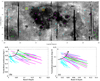 |
Fig. 2 (a) M3 global albedo mosaic (1578 nm) of 20 pixels per degree resolution and location of selected fresh craters. Craters from mare regions are shown in magenta circles and craters from highlands and highland-mare boundaries in cyan triangles. Crater from the South Pole Aitken (SPA) basin are shown as green triangles. The symbols do not represent the actual crater size. The locations marked by yellow squares belong to fresh craters considered for extracting representative spectra in Fig. 1. (b and c) Regression line fit to samples extracted from the locations shown in (a). The best fit regression lines are color coded as in (a) in the normalized continuum slope vs. band depth plots. The continuum slopes of band I and II were normalized to the 0.75 and 1.57 μm reflectances, respectively. Points following a line contain a constant abundance of Fe. The lines are oriented approximately radially with respect to the hypothetical “hypermature” reference point. A larger radial distance from the reference point correspond to fresher material. The definition of the angular parameters is according to Eq. (1) and shown here by an arrow. |
2.1.2 Application of MLR
When applying the technique of multivariate regression, we used the relation
 (2)
(2)
where Y is a matrix of size na × np that contains the LP GRS or KGRS elemental abundances, na is equal to the number of elements considered, and np is the number of LP GRS or KGRS pixels at 0.2 pixels per degree resolution. The matrix X contains the maturity-independent spectral parameters of the M3 mosaic in the same order as the LP GRS or KGRS data. The number of spectral parameters is denoted by nf, where in the case of nonlinear polynomial regression the higher-order multiplicative combinations of the different parameters would be considered as new parameters. Equation (2) is solved for the matrix C in the least-mean-squares sense. The correspondingly inferred matrix C can then be applied to 20 pixels per degree or full resolution M3 spectral parameter maps in order to estimate the corresponding elemental abundances using Eq. (2).
For the element Fe, a linear multivariate regression was performed. We found that the correlation of estimated Fe wt.% derived from Eq. (2) using the combination of maturity-independent spectral parameters with LP GRS Fe wt.% increases from 90 to 93% when the contribution of Fe contained in oxides, in particular ilmenite, is included. The approach of estimating the total Fe content by adding Fe contained in silicates andoxides was first proposed by Le Mouélic et al. (2000). It can be motivated by the fact that Fe contained in ilmenite has no influence on the depth or shape of band I and band II. The mineral ilmenite (FeTiO3), which is the most abundant oxide mineral found in lunar rocks, is present in significant amounts in some mare areas and can be included into the total iron content by adding 1.167 times the Ti wt.% value to the Fe wt.% estimated from regression analysis, where the factor 1.167 is the ratio between the atomic masses of Fe (56 amu) and Ti (48 amu). Similarly, a correction of 0.9 times the TiO2 wt.% value was estimated empirically by Le Mouélic et al. (2000) for the FeO wt.% estimation using Clementine multispectral VIS-NIR observations and by Bhatt et al. (2015) using M3 data. Interestingly, the empirically derived value of 0.9 is in very good agreement with the value expected from the stoichiometrical point of view, that is, the ratio between the molecular masses of the oxides FeO (72 amu) and TiO2 (80 amu) that form an ilmenite molecule.
We also applied the approach of including the contribution of Fe contained in oxides to KGRS Fe wt.%, using the Ti wt.% estimated with the M3-based regression approach of Bhatt et al. (2015). That method uses a quadratic polynomial regression approach for estimating the Ti abundance by performing a regression analysis between the LP GRS derived Ti abundance and two spectral parameters, that is, the continuum slope of band I (CSL1) and the logarithm of the ratio of BD1 and BD2, termed LBD. We found that the cross-correlation between the estimated and the LP GRS Tiabundance is 92% when considering only CSL1 and LBD as spectral parameters. This cross-correlation could not be improved by considering a combination of the maturity-independent parameters used for the other elements. Therefore, we used a global Ti abundance map obtained from Bhatt et al. (2015) to correct the estimated Fe abundances for Fe contained in ilmenite.
The proposed MLR model is applied to estimate the abundance of Ca by considering the same M3 spectral parameters and the LP GRS and KGRS Ca global maps. The Mg estimation uses the LP GRS Mg global map as reference. The obtained cross-correlation between reference maps and obtained estimation is 90% for Mg and 71% for Ca.The residual root mean square error (RMSE) is below 1 wt.% for the estimated Fe, Ca and Mg abundances.
2.1.3 Application of SVR
The technique of SVR is a commonly used non-parametric, kernel-based regression technique. An introduction to SVR is given, for instance,by Marsland (2015). SVR is an extension of the concept of support vector machine classification used for binary classification tasks. A vector of “input features” (here: the spectral parameters) is transformed into a higher-dimensional space, aiming at a transformation of the generally nonlinear relationship between the feature vectors and the target values (here: the GRS-based elemental abundances) into a linear (or less strongly nonlinear) one. To obtain an estimate of the target value for an arbitrary input feature vector, a pre-defined kernel function is applied to the scalar products between the input feature vector and a subset of all feature vectors used for training, the so-called support vectors. In practical applications, kernel functions of polynomial, sigmoid or Gaussian form are commonly used (Marsland 2015).
The estimated target value provided by SVR is obtained based on a weighted sum of the outputs of the kernel function applied to the scalar products between the input feature vector and all support vectors. Training the SVR corresponds to determining the set of support vectors along with a set of Lagrange multipliers, employing a quadratic programming based optimization. The error function minimized during SVR training is not quadratic but is represented by a nonnegative function that is zero if the training error, that is, the absolute difference between estimated and true target value, of the input feature vector is smaller than a pre-defined threshold ϵ, and linearly increases with the training error otherwise (Marsland 2015). Hence, a perfect SVR solution is obtained when the support vectors are chosen such that all training samples generate estimates that fall within the “tube” of 2ϵ width around the target values, whereas values outside the tube are allowed but the corresponding error function is minimized during the training procedure (Marsland 2015).
In this work we use the Matlab implementation of SVR configured with a Gaussian kernel function. For each of the elements Fe, Mg and Ca and each set of corresponding GRS “ground truth” (LP GRS and KGRS), one separate SVR is trained.
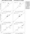 |
Fig. 3 Estimated vs. sample-based elemental abundances for Apollo and Luna landing sites, obtained by the MLR and SVR models. The LP GRS elemental maps of Fe, Ca, and Mg have been used as a reference for the MLR and SVR models. Thesample-based elemental compositions were taken from Elphic et al. (2000). The obtained RMSE values are listed along with the graphs. |
2.2 Validation of MLR and SVR models at landing sites
One of the main advantages of the proposed MLR and SVR models is use of LP GRS/KGRS global elemental maps as a reference. A large number of sample points and a broad range of compositional variations results in high prediction capabilities. However, LP GRS/KGRS elemental estimations rely heavily on pre-processing steps that might lead to systematic errors in the GRS-based elemental abundance estimations. Since the proposed algorithm uses GRS-based global maps as a reference, such errors will be inherent in the MLR and SVR models. Therefore, as an independent test we validate the newly developed algorithms at the Apollo and Luna landing sites by comparing the estimated abundances of Fe, Ca, and Mg with laboratory-based measurements. For this purpose, we applied the MLR and SVR models to M3 mosaics at full resolution of the sample-return missions Apollo 11, 12, 14-17 and Luna 16, 20, and 24 landing sites. The averaged sample-based landing site specific elemental abundances have been taken from Elphic et al. (2000). Figures 3 and 4 show MLR and SVR models applied to M3 mosaics of landing sites by considering LP GRS and KGRS data as a reference, respectively. The element-wise RMS deviations between sample-based and estimated abundances are also included in the plots. We found better correspondences for the KGRS-based Ca estimates than for the LP GRS based estimates, whereas the case is vice versa for the Fe estimates. It should be noted that the returned samples cover Mg and Ca contents in a relatively narrow value range when compared to the broad range available for the Fe content.
3 Results and discussion
3.1 Comparison with previous work on local scales
In this section we describe results obtained on local scales and compare them to previously published methods (Lucey et al. 2000b; Wöhler et al. 2014; Bhatt et al. 2015). Figures 5 and 6 illustrate a comparative analysis of the estimated Fe abundance on local scales. The calibration of our method based on LP GRS Fe data. For these regions, the results derived from MLR amd SVR models are nearly the same and therefore we included only MLR model Fe estimations.
The region shown in Fig. 5a is from crater Lichtenberg and surroundings located in the western part of Oceanus Procellarum. We selected the region east of the crater Lichtenberg for our comparative study (Fig. 5b). The selectedarea includes a boundary region between high-Ti and low-Ti mare, as well as several younger craters as evident from the Clementine-derived ratio mosaic (Lucey et al. 2000c) in Fig. 5c. This site is a good test-bed for studying small-scale variations and validating our new regression based-model at the compositionally varying basalt flows. The youngest basalt deposits in this region have been reported to be less around 1.5 Ga in age (Hiesinger et al. 2003).
The area shown in Fig. 6a corresponds to the crater Pierazzo and its neighborhood to the east on the lunar farside. The region shown in Fig. 6b includes mainly a wispy ray system east of the crater Pierazzo. The differences in albedo observed in Fig. 6 are due to immature material deposited on top of the mature background as a result of the impact that formed the crater Pierazzo.
The maturity-independent multivariate regression model is found to be the least sensitive to surface albedo and to topography induced effects that are otherwise prominent. The range and distribution of the Fe variation is similar and the boundary of low-and-high-Ti is detectable using all four algorithms of iron estimation as shown in Figs. 5d–g. The iron content of fresh craters derived using the algorithm of Bhatt et al. (2015) in Fig. 5d is 4–8 wt.% less than the surrounding mare, suggesting that the empirical calibration therein, which was applied based on the band depth vs. continuum slope relationship of one fresh crater which has a specific mare basalt composition, does not necessarily fit globally and would result in an underestimation of Fe at fresh crater locations. This difference is prominent mainly at highland locations, as evident from Fig. 6c. The Fe content of the ray system in Fig. 6c is lower by 1–2 wt.% in comparison to the surrounding surface, according to the band II based algorithm ofBhatt et al. (2015). The algorithm of Wöhler et al. (2014) estimates a 2–4 wt.% higher Fe content for fresh craters than for the surrounding surface in mare as well as in highland regions, suggesting a dependence on soil maturity (Figs. 5e and 6d). Small structures and fresh craters are largely removed in the iron maps derived by applying the algorithm of Lucey et al. (2000b) to the Clementine data, but topography effects are clearly visible in the highland region (Figs. 5f and 6e).
In contrast, the Fe abundance map obtained by the MLR model calibrated to LP GRS data neither shows maturity-related nor topographic artifacts in Figs. 5g and 6f.
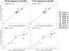 |
Fig. 4 Estimated vs. sample-based elemental abundances for Apollo and Luna landing sites by using MLR and SVR models. The KGRS elemental maps of Fe and Ca have been used as a reference for the MLR and SVR models. The sample based elemental compositions were taken from Elphic et al. (2000). The obtained RMSE values are listed along with the graphs. |
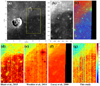 |
Fig. 5 (a) Lunar Reconnaissance Orbiter (LRO) Wide Angle Camera (WAC) mosaic (Speyerer et al. 2011) of the crater Lichtenberg and surroundings. The yellow box outline the region considered for obtaining Fe abundances using different approaches. (b) Full resolution M3 mosaic of the region east of the crater Lichtenberg. (c) Clementine UV/VIS color ratio mosaic (R channel: 750/415 nm, G channel: 750/1000 nm and B channel: 415/750 nm; Pieters et al. 1994) at 200 m/pixel spatial resolution. The low-titanium regions appear in red and yellow and the high-titanium regions appear in blue. (c)–(g) Derived Fe abundance using four different methods. The algorithm of Lucey et al. (2000b) was applied to Clementine UV/VIS data at 100 m/pixel spatial resolution. The dark region is due to a data gap in one of the Clementine bands. The algorithm of Bhatt et al. (2015) estimates a low Fe content for fresh craters, whereas the algorithm of Wöhler et al. (2014) tends to estimate a high Fe content for them. In contrast, small fresh do not appear as small-scale anomalies in the Fe abundance map obtained by the proposed MLR approach considering LP GRS as a reference. |
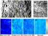 |
Fig. 6 (a) LRO WAC mosaic (Speyerer et al. 2011) of the crater Pierazzo and surroundings. The yellow box outlines the region considered for obtaining the Fe abundances using different approaches. (b) Full resolution M3 mosaic of the region east of the crater Pierazzo. (c)–(f) Fe abundance derived using four different methods. The algorithm of Lucey et al. (2000b) was applied to Clementine UV/VIS data at 100 m/pixel spatial resolution. The prominent ray structures are visible in the Fe abundance maps derived using the algorithms of Bhatt et al. (2015) and Wöhler et al. (2014) but are indistinguishable from the surroundingsurface in the Fe abundance map derived using the proposed MLR approach considering LP GRS as a reference. |
3.2 Comparison between the regression models at global scale
For the purpose of global elemental mapping, we used our M3 mosaic of 20 pixels per degree resolution. For our comparative analysis we constructed a total of four sets of global elemental maps using LP GRS and KGRS elemental abundance data as a reference, applying the MLR and SVR models to the global M3 mosaic. Themain focus here is to compare the results of the MLR and SVR models. Our elemental maps have been derived considering GRS observations as a ground truth which can probe the lunar surface up to about 20 cm depth (Feldman et al. 1999)with a spatial extent of tens to hundreds of kilometers (Lawrence et al. 1998). In contrast, the VIS-NIR spectrometers sample only the uppermost surface layer with a comparatively high spatial resolution of tens to hundreds of meters (Nozette et al. 1994; Pieters et al. 2009). Hence, a direct comparison between the elemental maps derived using GRS and VIS-NIR spectrometers would have to account for localized variations. The proposed regression models extend the approach of Wöhler et al. (2014) to elemental abundance estimation based on M3 observations by includingthe angular parameters defined in Eq. (1) as inputs to the model. The angular parameters have been computed from a M3 mosaic of 20 pixels per degree resolution in a similar way as suggested by Lucey et al. (2000b) but in a different parameter space as describedin Sect. 2. As a result, we observed that the elemental maps of Figs. 7–9 do not show dependencies on immature soil even for regions with high OMAT indices. As an example, the ray system of the crater Tycho (43° S, 11.36° W) is nearly absent in the Fe, Mg and Ca global maps (Figs. 7 and 8). The crater rim of Tycho exhibits a 2–3 wt.% increase in Ca and decrease in Mg content, presumably due to excavated material from the lower crust of chemically different composition. Tycho’s floor appears Fe-rich compared to the surrounding low-Fe highlands. We observed that the large bright ray systems in the farside highlands are absent in all cases discussed above, and small fresh cratersdo not introduce spurious anomalies of the elemental abundances. All the global maps clearly reflect the compositional differences between maria and highlands. Additionally, the compositional variations among different mare regions and mare-highland boundary regions are clearly distinguishable. The overall variations within the global elemental maps are comparable for Fe and Ca when either LP GRS or KGRS data are used as a reference.
In our new Fe maps, the highlands have iron abundances in the range 3–5 wt.% and maria in the range 16–22 wt.%. These values are within the range of published iron maps (Lucey et al. 2000b; Lawrence et al. 2002; Otake et al. 2012). The KGRS-calibrated Fe abundance map shown in Figs. 9a and c indicates a systematically lower estimated Fe abundance when compared to the LP GRS-calibrated Fe maps (Figs. 7 and 8). This discrepancy is likely to be due to slight systematic differences between the KGRS and LP GRS Fe maps (Naito et al. 2018). The Ca maps derived from LP GRS and KGRS data shown in Figs. 7–9 are comparable to within 1 wt.% deviation.
The Fe,Mg, and Ca estimates derived by the MLR and SVR models considering LP GRS as a reference are comparable in all regions except at the pyroclastic deposits of Sulpicius Gallus (19° N, 11° E) and Mare Vaporum (13° N, 4° E) (Carter et al. 2009) as well as the northwestern parts of Oceanus Procellarum (18° N, 57° W) known to berich in olivine (Zhang et al. 2016). In these regions, the MLR-based maps show enrichments of Fe and Mg and depletions of Ca. These anomalies are not apparent in the maps constructed with the SVR model, which indicates that they probably correspond to extrapolation artifacts of the MLR model due to the fact that the combinations of spectral parameters encountered in the pyroclastic deposits do not occur on larger spatial scales resolved by the GRS data used for calibration. Apparently, the SVR model better constrains the elemental abundances in such “unusual” areas with spectral properties that were “unknown” while adapting the regression models. Furthermore, the Mg map derived using the SVR model in Fig. 8 shows the well-known noritic anomaly in the Mare Frigoris (56° N, 1° E) region (Isaacson & Pieters 2009) more distinctly in comparison to the MLR-derived Mg map in Fig. 7.
The Ca and Mg global maps in Figs. 7 and 8 do not correlate strongly with the Fe maps, with a correlation coefficient of~0.6. This indicates that the spectral parameters used for regression reveal independent information about Mg and Ca. Variations in the Mg and Ca abundances are in part due to variations in the abundances of the minerals orthopyroxene and clinopyroxene. The presence of non-transition Ca2+ and/or Mg2+ cations along with the transition element Fe2+ in the pyroxene series is responsible for changes in the crystal lattice distances. The lattice distance corresponds to a shift towards longer wavelengths in the band I and band II domains with increasing content of Ca2+ cations (Burns 1993; Klima et al. 2011). The low-Ca regions in Fig. 7 therefore correspond to the nearside and farside maria and the South Pole-Aitken Basin, where variations across the maria are visible that correspond to basalts dominated by clinopyroxene (high Ca, low Mg) vs. orthopyroxene (low Ca, high Mg). What is more, for lunar minerals the weakness or absence of band I and band II indicates plagioclase, which has a relatively high Ca content when compared to the pyroxene-rich maria. Hence, although there is not one single spectral parameter that indicates the Ca and Mg abundances in lunar minerals, a combination of band depths and center wavelengths is apparently able to provide such information. Multivariate regression techniques like those used in this study are ideal for extracting such information from a multidimensional space of spectral parameters.
The Mg and Ca abundances in South Pole-Aitken (SPA) are similar to those in the nearside maria, whereas the Fe content differs by a factor of about two. Another such location belong to the Northern Imbrium Noritic (NIN) anomaly (55° N to 75° N and 85° W to 5° E) (Isaacson & Pieters 2009) which corresponds to an extended high-Mg and low-Ca area that exhibits only a weak contrast to Mare Frigoris. The basalts of Mare Frigoris have a significantly higher Fe content than the surrounding highland areas particularly in Fig. 8. As an another example of independent variations in Fe, Mg and Ca, we derived elemental maps of Mare Serenitatis in Fig. 10. The Ca map of Mare Serenitatis shows high-Ca basalt, presumably clinopyroxene, in the western, northern and easternmost part of the mare and near the southern border. In contrast, the central part consists of basalts with a lower Ca content. The high-Ca basalt in northwestern Mare Serenitatis has been identified by Grumpe et al. (2018) as a topographically apparent flow unit of high-Ca basalt overlying a larger unit of low-Ca basalt. The well-known pyroclastic deposit near Sulpicius Gallus at the southwestern border of Mare Serenitatis appears as a low-Ca and high-Mg area. The variations in Fe content across Mare Serenitatis do not correlate strongly with the variations in Mg and Ca. Notably, none of the three elemental abundance maps shows anomalies near fresh craters in Mare Serenitatis, such as Linné (27.7° N, 11.8° E) or Bessel F (21.2° N, 13.8° E) and G (21.1° N, 14.7° E).
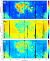 |
Fig. 7 M3-derived global elemental maps using LP GRS elemental abundance data as reference. (a) Fe, (b) Ca, and (c) Mg. The maps were constructed using the MLR model. |
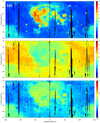 |
Fig. 8 M3-derived global elemental maps using LP GRS elemental abundance data as a reference. (a) Fe, (b) Ca, and (c) Mg. The maps were constructed using the SVR model. |
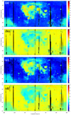 |
Fig. 9 M3-derived global elemental maps of (a) Fe and (b) Ca using the MLR model and KGRS elemental abundance data as a reference, (c) Fe and (d) Ca using the SVR model and KGRS elemental abundance data as a reference. |
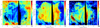 |
Fig. 10 Elemental abundance maps of Mare Serenitatis using the MLR model and LP GRS elemental abundance data as a reference. The variations in the Ca and Mg maps are independent of the Fe map. |
4 Conclusion
The MLR analysis allows us to map the abundances of the elements Fe, Mg and Ca at a typical accuracy of about 1 wt.% at the spatial resolution of the M3 data. The proposed new algorithm requires global M3 spectral parameters map and LP GRS or KGRS global elemental data as an input to the MLR and SVR models. The main advantage of the proposed new algorithm is its ability to minimize the space-weathering effects. The new approach of estimating elemental abundances based on MLR and SVR models combines the advantages of the previously proposed algorithms of Wöhler et al. (2014) and Bhatt et al. (2015) with those of Lucey et al. (2000b). The site-specific studies indicate that effects of topography and maturity have been significantly reduced and do not introduce artifacts into the elemental abundance maps. The results derived using the MLR and SVR models are comparable at the Apollo and Luna sample-return sites. However, when applied at global scale the MLR-derived elemental maps show small-scale anomalies at pyroclastic deposits. The Ca and Mg global distributions derived in this work do not correlate strongly with the Fe maps. We conclude that the spectral parameters used and models developed in this work successfully minimize the space-weathering effects on the spatial scale of the M3 observations and reveal Fe-independent information about Mg and Ca and thus on the lunar surface chemistry.
The global elemental abundance maps derived for the fully calibrated M3 global dataset would be of high interest for estimating quantitative geochemical information. These maps will serve as important tools to investigate the lunar geologic evolution. Future work will focus on site-specific studies based on detected elemental abundance anomalies and on the preparation of petrological maps using our derived elemental maps. This approach is mainly useful for detailed geologic mapping of study regions on the Moon. Furthermore, our high-resolution elemental maps will be of interest for future lander missions in the context of landing site selection. In situ observations from already planned lander and rover missions such as Chandrayaan-2 (Bagla 2018) will provide opportunities to further validate the developed elemental abundance estimation methods. With future missions planned for lunar and asteroid explorations, the methodology developed for global elemental estimation independent of maturity holds importance in understanding of planetary formation and evolution, and space resource utilization.
Digital versions of the nearly global elemental abundance maps are available online1.
Acknowledgements
The authors wish to thank Dr. Stéphane Le Mouélic for his helpful review of the manuscript. We downloaded the Moon Mineralogy Mapper (https://pds-imaging.jpl.nasa.gov/volumes/m3.html), Lunar Prospector (https://www.mapaplanet.org/explorer/moon.html), Kaguya (https://darts.isas.jaxa.jp/planet/pdap/selene/), Clementine (https://astrogeology.usgs.gov/search/map/Moon/Clementine/UVVIS/Lunar_Clementine_UVVIS_WarpMosaic_5Bands_200m) and LRO (http://wms.lroc.asu.edu/lroc/view_rdr/WAC_GLOBAL) datasets from the public domain and acknowledge the respective teams for maintaining the data portals. This work was partially supported by a DAAD fellowship for “Research Stays for University Academics and Scientists, 2017”. M.B. was supported by Department of Space, Government of India.
Appendix A Global Ti map
The global Ti wt.% map in Fig. A.1 was derived using the method described by Bhatt et al. (2015). This Ti wt.% estimation is being used for estimating the total Fe wt.% considering the LP GRS and KGRS global elemental abundance data as a reference. The M3 -derived Ti distribution in Fig. A.1 follows the LP GRS-derived Ti wt.% with a maximum content of up to ~ 6 wt.%, whereas the Clementine-derived Ti content may reach up to ~10 wt.% (Lucey et al. 2000b). While the Ti distributions derived from M3 and Clementine are broadly comparable and in good agreement in most areas, there are significant discrepancies at some locations. These discrepancies are strongest at the pyroclastic deposits of Rima Bode, Mare Vaporum, Mare Serenitatis and Sinus Aestuum, where the Clementine-derived Ti abundances are extraordinarily high. This behavior might be due to the fact that the ratio method of Lucey et al. (2000b) does not apply to Wilcox et al. (2006).
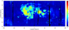 |
Fig. A.1 M3-derived global Ti map derived using the method described by Bhatt et al. (2015). The global LP GRS Ti distribution has been considered as a reference. |
Appendix B Residual maps at global scale based on MLR and SVR models
A set of all combinations of residual maps based on the MLR and SVR models are shown in Figs. B.1–B.3. The corresponding RMSE values are also listed along with the graphs. The residual maps highlights differences present due to two different models applied to the calibrated set of M3 observationsusing the LP GRS and KGRS elemental abundances as reference. The difference maps obtained for the MLR and SVR models show maximum differences of about 5 wt.% for Fe and Mg in small areas but mostly not more than 2 wt.%. The maximum difference for the Ca maps is about 2 wt.%. The regions with maximum elemental difference are located mainly at the pyroclastic deposits, Northern Imbrium Noritic (NIN) anomaly, Mare Imbrium, Oceanus Procellarum, Mare Humorum, Mare Australe, Mare Serenitatis, and in SPA. The difference in elemental abundance for the low-latitude highlands is below 1 wt.% but increases to 2 wt.% for high latitude highlands. The residual deviations are reduced in the case where the SVR model has been applied to estimate Fe and Ca. Such a comparison cannot be carried out for the Mg estimation due to unavailability of a global KGRS Mg map.
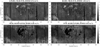 |
Fig. B.1 Residual maps of Fe abundances using MLR and SVR models and LP GRS and KGRS as a reference. |
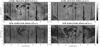 |
Fig. B.2 Residual maps of Ca abundances using MLR and SVR models and LP GRS and KGRS as a reference. |
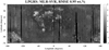 |
Fig. B.3 Residual map of Mg abundances using MLR and SVR models and LP GRS as a reference. |
Appendix C Global maps of iron sensitive parameters
The global maps of iron sensitive parameters, A1 and A2 have been derived using Eq. (1). We have compared variations in A1 and A2 with the iron sensitive parameter of Lucey et al. (2000b) derived using the Clementine global mosaic in Fig. C.1. The iron sensitive parameter θFe is derived using following relation (Lucey et al. 2000b):
![\begin{equation*}\theta_{\textrm{Fe}}=-\arctan{[(R_{950}/R_{750})-y_{\textrm{0Fe}}]/[R_{750}-x_{\textrm{0Fe}}]}, \end{equation*}](/articles/aa/full_html/2019/07/aa35773-19/aa35773-19-eq3.png) (C.1)
(C.1)
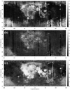 |
Fig. C.1 Global maps of iron sensitive parameters derived using Eq. (1) compared with the iron sensitive parameter of Lucey et al. (2000b). The maps have been derived at spatial resolution of 1.5 km at equatorial region. The data gaps are shown in black color in M3 derived iron sensitive parameters and in white color in Clementine derived iron sensitive parameter. (a) A1 parameter; (b) A2 parameter; (c) the angular iron sensitive parameter derived using Eq. (C.1). It should be noted that the iron sensitive parameters derived in this work and from Lucey et al. (2000b) do not belong to the same coordinate space. For comparison purpose we have plotted here − θFe. |
where R950 and R750 denote the reflectances at 950 and 750 nm, x0Fe and y0Fe are reference point which serve as the origin for θFe. The coordinates of x0Fe and y0Fe are adjusted manually by Lucey et al. (2000b) and set to x0Fe = 0.08 and y0Fe = 1.19 in order to minimize the effect of optical maturity on the estimated FeO abundance.
We plotted − θFe in Fig. C.1c mainly for a visual comparison so that maria represented as bright and highlands represented as dark in all the three maps in Fig. C.1. We found that on a broad scale parameters A1 and A2 are comparable to θFe. Additionally, parameter A1 shows a clear discrimination between high-Ti and low-Ti basalts and parameter A2 highlights the pyroclastic deposits. The iron sensitive parameters derived in this work and from Lucey et al. (2000b) are comparable at the SPA basin.
References
- Bagla, P. 2018, India plans tricky and unprecedented landing near moon’s south pole, http://www.sciencemag.org/news/2018/01/india-plans- tricky-and-unprecedented-landing-near-moon-s-south-pole [Google Scholar]
- Barker, M. K., Mazarico, E., Neumann, G. A., et al. 2016, Icarus, 273, 346 [NASA ADS] [CrossRef] [Google Scholar]
- Bhatt, M., Mall, U., Bugiolacchi, R., et al. 2012, Icarus, 220, 51 [NASA ADS] [CrossRef] [Google Scholar]
- Bhatt, M., Mall, U., Wöhler, C., Grumpe, A., & Bugiolacchi, R. 2015, Icarus, 248, 72 [NASA ADS] [CrossRef] [Google Scholar]
- Blewett, D. T., Lucey, P. G., Hawke, B. R., & Jolliff, B. L. 1997a, J. Geophys. Res., 102, 16319 [Google Scholar]
- Blewett, D. T., Lucey, P. G., Hawke, B. R., & Jolliff, B. L. 1997b, Lunar Planet. Sci. Conf., 28, 121 [NASA ADS] [Google Scholar]
- Burns, R. G. 1993, Mineralogical Applications of Crystal Field Theory, 2nd edn. (New York: Cambridge University Press) [CrossRef] [Google Scholar]
- Carter, L. M., Campbell, B. A., Hawke, B. R., Campbell, D. B., & Nolan, M. C. 2009, J. Geophys. Res. Planets, 114, E11004 [NASA ADS] [CrossRef] [Google Scholar]
- Crawford, I. A., Joy, K. H., Kellett, B. J., et al. 2009, Planet. Space Sci., 57, 725 [NASA ADS] [CrossRef] [Google Scholar]
- Elphic, R. C., Lawrence, D. J., Feldman, W. C., et al. 1998, Science, 281, 1493 [NASA ADS] [CrossRef] [Google Scholar]
- Elphic, R., Lawrence, D., Feldman, W., et al. 2000, J. Geophys. Res. Planets, 105, 20333 [NASA ADS] [CrossRef] [Google Scholar]
- Feldman, W. C., Barraclough, B. L., Fuller, K. R., et al. 1999, Nucl. Instrum. Methods Phys. Res. A., 422, 562 [NASA ADS] [CrossRef] [Google Scholar]
- Fischer, E. M., & Pieters, C. M. 1996, J. Geophys. Res., 101, 2225 [NASA ADS] [CrossRef] [Google Scholar]
- Fu, Z., Robles-Kelly, A., Caelli, T., & Tan, R. T. 2007, IEEE Trans. Geosci. Remote Sens., 45, 3827 [NASA ADS] [CrossRef] [Google Scholar]
- Gillis, J. J., Jolliff, B. L., & Korotev, R. L. 2004, Geochim. Cosmochim. Acta, 68, 3791 [NASA ADS] [CrossRef] [Google Scholar]
- Grumpe, A., & Wöhler, C. 2014, ISPRS J. Photogramm. Remote Sens., 94, 37 [NASA ADS] [CrossRef] [Google Scholar]
- Grumpe, A., Belkhir, F., & Wöhler, C. 2014, Adv. Space Res., 53, 1735 [NASA ADS] [CrossRef] [Google Scholar]
- Grumpe, A., Wöhler, C., Rommel, D., Bhatt, M., & Mall, U. 2018, in Planetary Remote Sensing and Mapping, eds. B. Wu, K. Di, J. Oberst, & I. Karachevtseva (Leiden: CRC Press) [Google Scholar]
- Grumpe, A., Wöhler, C., Berezhnoy, A. A., & Shevchenko, V. V. 2019, Icarus, 321, 486 [NASA ADS] [CrossRef] [Google Scholar]
- Hapke, B. 1984, Icarus, 59, 41 [NASA ADS] [CrossRef] [Google Scholar]
- Hapke, B. 2001, J. Geophys. Res., 106, 10039 [NASA ADS] [CrossRef] [Google Scholar]
- Hapke, B. 2002, Icarus, 157, 523 [NASA ADS] [CrossRef] [Google Scholar]
- Hapke, B. 2012, Theory of Reflectance and Emittance Spectroscopy (Cambridge: Cambridge University Press) [Google Scholar]
- Hiesinger, H., Head, III, J., Wolf, U., Jaumann, R., & Neukum, G. 2003, J. Geophys. Res., 108, 5065 [CrossRef] [Google Scholar]
- Isaacson, P. J., & Pieters, C. M. 2009, J. Geophys. Res. Planets, 114, E09007 [NASA ADS] [CrossRef] [Google Scholar]
- Keller, L. P., & McKay, D. S. 1993, Science, 261, 1305 [NASA ADS] [CrossRef] [Google Scholar]
- Klima, R. L., Pieters, C. M., Boardman, J. W., et al. 2011, J. Geophys. Res. Planets, 116, E00G06 [CrossRef] [Google Scholar]
- Kramer, G. Y., Jolliff, B. L., & Neal, C. R. 2008, J. Geophys. Res. Planets, 113, 1002 [NASA ADS] [CrossRef] [Google Scholar]
- Lawrence, D. J., Feldman, W. C., Barraclough, B. L., et al. 1998, Science, 281, 1484 [NASA ADS] [CrossRef] [Google Scholar]
- Lawrence, D. J., Feldman, W. C., Elphic, R. C., et al. 2002, J. Geophys. Res. Planets, 107, 5130 [NASA ADS] [CrossRef] [Google Scholar]
- Le Mouélic, S., Langevin, Y., & Erard, S. 1999, Geophys. Res. Lett., 26, 1195 [NASA ADS] [CrossRef] [Google Scholar]
- Le Mouélic, S., Langevin, Y., Erard, S., et al. 2000, J. Geophys. Res., 105, 9445 [NASA ADS] [CrossRef] [Google Scholar]
- Le Mouélic, S., Lucey, P. G., Langevin, Y., & Hawke, B. R. 2002, J. Geophys. Res. Planets, 107, 5074 [NASA ADS] [CrossRef] [Google Scholar]
- Lucey, P. G. 2006, J. Geophys. Res. Planets, 111, 8003 [NASA ADS] [CrossRef] [Google Scholar]
- Lucey, P. G., Taylor, G. J., & Malaret, E. 1995, Science, 268, 1150 [NASA ADS] [CrossRef] [Google Scholar]
- Lucey, P. G., Blewett, D. T., & Hawke, B. R. 1998, J. Geophys. Res., 103, 3679 [Google Scholar]
- Lucey, P. G., Blewett, D. T., Eliason, E. M., et al. 2000a, LPI Sci. Conf. Abstr., 31, 1273 [Google Scholar]
- Lucey, P. G., Blewett, D. T., & Jolliff, B. L. 2000b, J. Geophys. Res., 105, 20297 [Google Scholar]
- Lucey, P. G., Blewett, D. T., Taylor, G. J., & Hawke, B. R. 2000c, J. Geophys. Res., 105, 20377 [Google Scholar]
- Mall, U., Banaszkiewicz, M., Bronstad, K., et al. 2009, Curr. Sci., 96, 506 [Google Scholar]
- Marsland, S. 2015, Machine Learning: An Algorithmic Perspective, 2nd edn. (New Jersey, USA: CRC Press) [Google Scholar]
- McKay, D., Heiken, G., Basu, A., et al. 1991, in Lunar Sourcebook, eds. G. H. Heiken, D. T. Vaniman, & B. M. French (New York: Cambridge University Press), 285 [Google Scholar]
- Naito, M., Hasebe, N., Nagaoka, H., et al. 2018, Icarus, 310, 21 [NASA ADS] [CrossRef] [Google Scholar]
- Nozette, S., Rustan, P., Pleasance, L. P., et al. 1994, Science, 266, 1835 [NASA ADS] [CrossRef] [Google Scholar]
- Otake, H., Ohtake, M., & Hirata, N. 2012, LPI Sci. Conf. Abstr., 43, 1905 [Google Scholar]
- Pieters, C. M. 1999, Proc. Workshop on New Views of the Moon II, abstract #8025 [Google Scholar]
- Pieters, C. M., Staid, M. I., Fischer, E. M., Tompkins, S., & He, G. 1994, Science, 266, 1844 [NASA ADS] [CrossRef] [Google Scholar]
- Pieters, C. M., Taylor, L. A., Noble, S. K., et al. 2000, Meteorit. Planet. Sci., 35, 1101 [NASA ADS] [CrossRef] [Google Scholar]
- Pieters, C., Boardman, J., Buratti, B., et al. 2009, Curr. Sci., 96, 500 [Google Scholar]
- Prettyman, T. H., Hagerty, J. J., Elphic, R. C., et al. 2006, J. Geophys. Res. Planets, 111, 12007 [NASA ADS] [CrossRef] [Google Scholar]
- Shkuratov, Y. G., Kaydash, V. G., Stankevich, D. G., et al. 2005, Planet. Space Sci., 53, 1287 [NASA ADS] [CrossRef] [Google Scholar]
- Shkuratov, Y., Kaydash, V., Korokhin, V., et al. 2011, Planet. Space Sci., 59, 1326 [NASA ADS] [CrossRef] [Google Scholar]
- Speyerer, E. J., Robinson, M. S., & Denevi, B. W. 2011, LPI Sci. Conf. Abstr., 42, 2387 [Google Scholar]
- Taylor, L. A., Pieters, C. M., Keller, L. P., Morris, R. V., & McKay, D. S. 2001, J. Geophys. Res., 106, 27985 [NASA ADS] [CrossRef] [Google Scholar]
- Wilcox, B. B., Lucey, P. G., & Gillis, J. J. 2005, J. Geophys. Res. Planets, 110, E11001 [NASA ADS] [CrossRef] [Google Scholar]
- Wilcox, B. B., Lucey, P. G., & Hawke, B. R. 2006, J. Geophys. Res. Planets, 111, E09001 [NASA ADS] [CrossRef] [Google Scholar]
- Wöhler, C., Berezhnoy, A., & Evans, R. 2011, Planet. Space Sci., 59, 92 [NASA ADS] [CrossRef] [Google Scholar]
- Wöhler, C., Grumpe, A., Berezhnoy, A., Bhatt, M. U., & Mall, U. 2014, Icarus, 235, 86 [NASA ADS] [CrossRef] [Google Scholar]
- Wöhler, C., Grumpe, A., Berezhnoy, A. A., et al. 2017a, Icarus, 285, 118 [NASA ADS] [CrossRef] [Google Scholar]
- Wöhler, C., Grumpe, A., Berezhnoy, A. A., & Shevchenko, V. V. 2017b, Sci. Adv., 3, e1701286 [NASA ADS] [CrossRef] [Google Scholar]
- Wu, Y., Xue, B., Zhao, B., et al. 2012, J. Geophys. Res. Planets, 117, 2001 [NASA ADS] [Google Scholar]
- Xia, W., Wang, X., Zhao, S., et al. 2019, Icarus, 321, 200 [NASA ADS] [CrossRef] [Google Scholar]
- Yamashita, N., Gasnault, O., Forni, O., et al. 2012, Earth Planet. Sci. Lett., 353–354, 93 [NASA ADS] [CrossRef] [Google Scholar]
- Zhang, X., Wu, Y., Ouyang, Z., et al. 2016, J. Geophys. Res. Planets, 121, 2063 [NASA ADS] [CrossRef] [Google Scholar]
All Figures
|
Fig. 1 Representative spectra of fresh crater locations from highland and mare regions and their respective band depth vs. continuum slope trends. The fresh crater locations from highland and mare region are marked as yellow squares in Fig. 2. (a) Reflectance spectra extracted from the interior to the outer rim of the ejecta blanket in sequence to demonstrate the decrease in band depth with increasing maturity. (b) Continuum-removed reflectance spectra of (a), clearly showing gradual changes in band depth as we move gradually away from a small crater. The representative spectra of highland in this case are offset by 0.03 for a clear representation. (c, d) Normalized continuum slope vs. band depth plots for band I and band II, respectively, showing linear trends for fresh crater locations from highland and mare regions. Maturity increases towards higher normalized continum slope and lower band depth values. The continuum slopes of band I and band II were normalized to the 0.75 and 1.57 μm reflectances,respectively. |
| In the text | |
|
Fig. 2 (a) M3 global albedo mosaic (1578 nm) of 20 pixels per degree resolution and location of selected fresh craters. Craters from mare regions are shown in magenta circles and craters from highlands and highland-mare boundaries in cyan triangles. Crater from the South Pole Aitken (SPA) basin are shown as green triangles. The symbols do not represent the actual crater size. The locations marked by yellow squares belong to fresh craters considered for extracting representative spectra in Fig. 1. (b and c) Regression line fit to samples extracted from the locations shown in (a). The best fit regression lines are color coded as in (a) in the normalized continuum slope vs. band depth plots. The continuum slopes of band I and II were normalized to the 0.75 and 1.57 μm reflectances, respectively. Points following a line contain a constant abundance of Fe. The lines are oriented approximately radially with respect to the hypothetical “hypermature” reference point. A larger radial distance from the reference point correspond to fresher material. The definition of the angular parameters is according to Eq. (1) and shown here by an arrow. |
| In the text | |
|
Fig. 3 Estimated vs. sample-based elemental abundances for Apollo and Luna landing sites, obtained by the MLR and SVR models. The LP GRS elemental maps of Fe, Ca, and Mg have been used as a reference for the MLR and SVR models. Thesample-based elemental compositions were taken from Elphic et al. (2000). The obtained RMSE values are listed along with the graphs. |
| In the text | |
|
Fig. 4 Estimated vs. sample-based elemental abundances for Apollo and Luna landing sites by using MLR and SVR models. The KGRS elemental maps of Fe and Ca have been used as a reference for the MLR and SVR models. The sample based elemental compositions were taken from Elphic et al. (2000). The obtained RMSE values are listed along with the graphs. |
| In the text | |
|
Fig. 5 (a) Lunar Reconnaissance Orbiter (LRO) Wide Angle Camera (WAC) mosaic (Speyerer et al. 2011) of the crater Lichtenberg and surroundings. The yellow box outline the region considered for obtaining Fe abundances using different approaches. (b) Full resolution M3 mosaic of the region east of the crater Lichtenberg. (c) Clementine UV/VIS color ratio mosaic (R channel: 750/415 nm, G channel: 750/1000 nm and B channel: 415/750 nm; Pieters et al. 1994) at 200 m/pixel spatial resolution. The low-titanium regions appear in red and yellow and the high-titanium regions appear in blue. (c)–(g) Derived Fe abundance using four different methods. The algorithm of Lucey et al. (2000b) was applied to Clementine UV/VIS data at 100 m/pixel spatial resolution. The dark region is due to a data gap in one of the Clementine bands. The algorithm of Bhatt et al. (2015) estimates a low Fe content for fresh craters, whereas the algorithm of Wöhler et al. (2014) tends to estimate a high Fe content for them. In contrast, small fresh do not appear as small-scale anomalies in the Fe abundance map obtained by the proposed MLR approach considering LP GRS as a reference. |
| In the text | |
|
Fig. 6 (a) LRO WAC mosaic (Speyerer et al. 2011) of the crater Pierazzo and surroundings. The yellow box outlines the region considered for obtaining the Fe abundances using different approaches. (b) Full resolution M3 mosaic of the region east of the crater Pierazzo. (c)–(f) Fe abundance derived using four different methods. The algorithm of Lucey et al. (2000b) was applied to Clementine UV/VIS data at 100 m/pixel spatial resolution. The prominent ray structures are visible in the Fe abundance maps derived using the algorithms of Bhatt et al. (2015) and Wöhler et al. (2014) but are indistinguishable from the surroundingsurface in the Fe abundance map derived using the proposed MLR approach considering LP GRS as a reference. |
| In the text | |
|
Fig. 7 M3-derived global elemental maps using LP GRS elemental abundance data as reference. (a) Fe, (b) Ca, and (c) Mg. The maps were constructed using the MLR model. |
| In the text | |
|
Fig. 8 M3-derived global elemental maps using LP GRS elemental abundance data as a reference. (a) Fe, (b) Ca, and (c) Mg. The maps were constructed using the SVR model. |
| In the text | |
|
Fig. 9 M3-derived global elemental maps of (a) Fe and (b) Ca using the MLR model and KGRS elemental abundance data as a reference, (c) Fe and (d) Ca using the SVR model and KGRS elemental abundance data as a reference. |
| In the text | |
|
Fig. 10 Elemental abundance maps of Mare Serenitatis using the MLR model and LP GRS elemental abundance data as a reference. The variations in the Ca and Mg maps are independent of the Fe map. |
| In the text | |
|
Fig. A.1 M3-derived global Ti map derived using the method described by Bhatt et al. (2015). The global LP GRS Ti distribution has been considered as a reference. |
| In the text | |
|
Fig. B.1 Residual maps of Fe abundances using MLR and SVR models and LP GRS and KGRS as a reference. |
| In the text | |
|
Fig. B.2 Residual maps of Ca abundances using MLR and SVR models and LP GRS and KGRS as a reference. |
| In the text | |
|
Fig. B.3 Residual map of Mg abundances using MLR and SVR models and LP GRS as a reference. |
| In the text | |
|
Fig. C.1 Global maps of iron sensitive parameters derived using Eq. (1) compared with the iron sensitive parameter of Lucey et al. (2000b). The maps have been derived at spatial resolution of 1.5 km at equatorial region. The data gaps are shown in black color in M3 derived iron sensitive parameters and in white color in Clementine derived iron sensitive parameter. (a) A1 parameter; (b) A2 parameter; (c) the angular iron sensitive parameter derived using Eq. (C.1). It should be noted that the iron sensitive parameters derived in this work and from Lucey et al. (2000b) do not belong to the same coordinate space. For comparison purpose we have plotted here − θFe. |
| In the text | |
Current usage metrics show cumulative count of Article Views (full-text article views including HTML views, PDF and ePub downloads, according to the available data) and Abstracts Views on Vision4Press platform.
Data correspond to usage on the plateform after 2015. The current usage metrics is available 48-96 hours after online publication and is updated daily on week days.
Initial download of the metrics may take a while.