| Issue |
A&A
Volume 627, July 2019
|
|
|---|---|---|
| Article Number | A74 | |
| Number of page(s) | 9 | |
| Section | Cosmology (including clusters of galaxies) | |
| DOI | https://doi.org/10.1051/0004-6361/201935548 | |
| Published online | 03 July 2019 | |
The case for two-dimensional galaxy–galaxy lensing
Leiden Observatory, Leiden University, PO Box 9513 2300 RA Leiden, The Netherlands
e-mail: This email address is being protected from spambots. You need JavaScript enabled to view it.
Received:
26
March
2019
Accepted:
28
May
2019
Abstract
We revisit the performance and biases of the two-dimensional approach to galaxy–galaxy lensing. This method exploits the information for the actual positions and ellipticities of source galaxies, rather than using only the ensemble properties of statistically equivalent samples. We compare the performance of this method with the traditionally used one-dimensional tangential shear signal on a set of mock data that resemble the current state-of-the-art weak lensing surveys. We find that under idealised circumstances the confidence regions of joint constraints for the amplitude and scale parameters of the NFW model in the two-dimensional analysis can be more than three times tighter than the one-dimensional results. Moreover, this improvement depends on the lens number density and it is larger for higher densities. We compare the method against the results from the hydrodynamical EAGLE simulation in order to test for possible biases that might arise due to lens galaxies being missed, and find that the method is able to return unbiased estimates of halo masses when compared to the true properties of the EAGLE galaxies. Because of its advantage in high galaxy density areas, the method is especially suitable for studying the properties of satellite galaxies in clusters of galaxies.
Key words: gravitational lensing: weak / methods: statistical / galaxies: halos / dark matter / large-scale structure of Universe / surveys
© ESO 2019
1. Introduction
One of the fundamental ingredients needed to understand galaxy formation is the relation between stellar mass and the host halo mass (e.g. Courteau et al. 2014). However, inferring the total mass from a galaxy’s emitted light is not feasible. We must instead rely on different probes to constrain the mass of dark matter haloes around galaxies one wants to study. A powerful mechanism that can be used for this is gravitational lensing, when matter inhomogeneities deflect light rays from distant objects along their path. As a consequence the images of distant objects (sources) appear to be tangentially distorted around foreground galaxies (lenses). The strength of the distortion is proportional to the amount of mass associated with the lenses (and consequently the dark matter haloes) and it is stronger in the proximity of the centre (for a thorough review, see Bartelmann & Schneider 2001).
Weak gravitational lensing induces a coherent tangential distortion. Under the assumption that galaxies are randomly oriented, the lensing signal can be inferred by simply averaging the ellipticities of the source galaxies. The typical change in ellipticity due to gravitational lensing is much smaller than the intrinsic ellipticity of the source, even in the case of clusters of galaxies. The weak gravitational lensing signal from a single galaxy halo is therefore too weak to be detected, and we must rely on a statistical approach in which the contributions from different lens galaxies are stacked, selected by similar observational properties (e.g. stellar masses, luminosities, size). The usual method used to analyse weak lensing data is to average the tangential component of the distortion in radial bins. As the signal from a single lens is purely tangential, this is a succinct way of showing the information contained in the distortions induced by one lens; there is no information lost in azimuthally averaging a radially symmetric signal and therefore the mass distribution of the lens can be perfectly determined from this radial profile. Average halo properties, such as halo masses, are then inferred from the resulting high signal-to-noise ratio measurements. This technique is commonly referred to as galaxy–galaxy lensing, and it is used as a method to measure statistical properties of dark matter haloes around galaxies (e.g. Leauthaud et al. 2011; van Uitert et al. 2011; Velander et al. 2014; Cacciato et al. 2014; Viola et al. 2015). The stacking mentioned here is not required per se, but it provides a convenient and unbiased data compression method that also allows for separate study of central and satellite galaxies. However, it does typically result in a loss of information about the halo properties.
For the lenses that do not exist in isolation the signal is not purely tangential. In this case the distortions around a lens are the sum of the tangential patterns of all the neighbouring lenses. An azimuthal average of these distortions will discard the azimuthal information that is present in this case. This non-optimal use of information will result in a less precise mass estimation than would be possible with a two-dimensional method.
Here we revisit a different method of analysing galaxy–galaxy lensing data, first proposed by Schneider & Rix (1997), and we make a case for why it should be considered again: it uses the unique signatures of overlapping regions of lenses to constrain the halo properties more precisely. Two-dimensional galaxy–galaxy lensing tries to fit a two-dimensional shear field directly to the galaxy ellipticity measurements. It was initially named “maximum-likelihood galaxy–galaxy lensing” after the fitting method it was first studied with (e.g. Schneider & Rix 1997; Hudson et al. 1998; Geiger & Schneider 1999; Hoekstra et al. 2003, 2004; Han et al. 2015). Maximum-likelihood galaxy–galaxy lensing is thus a misnomer and in principle one could use any form of fitting method to infer the desired parameters of the two-dimensional weak lensing maps, ideally using a fully Bayesian model (Sonnenfeld & Leauthaud 2018).
This method went out of fashion due to the unavailability of the galaxy grouping information that would accurately classify the galaxies as centrals and satellites (Hoekstra 2014) as it was realised that these objects need to be modelled separately. Treating the galaxies as centrals and satellites in a statistical way when considering the stacked signal could be naturally accounted for with the halo model (Seljak 2000; Peacock & Smith 2000; Cooray & Sheth 2002), thus overcoming the observational shortcomings. In recent years the galaxy grouping information has become available due to the power of wide-field photometric surveys (e.g. KiDS; Kuijken et al. 2015; de Jong et al. 2015) complemented with spectroscopic group information (from spectroscopic surveys like GAMA; Driver et al. 2011; Robotham et al. 2011) that treat the central and satellite galaxies deterministically (e.g. Sifón et al. 2015; Brouwer et al. 2017). One important advantage of the two-dimensional method is that it exploits all the information of the actual image configuration (the model predicts the shear for each individual galaxy image) using various parameters, including the galaxies’ exact positions, ellipticities, magnitudes, luminosities, stellar masses and group membership information rather than using only the ensemble properties of statistically equivalent samples (Schneider & Rix 1997). Moreover, the clustering of the lenses is naturally taken into account, although it is more difficult to account for the expected diversity in density profiles (Hoekstra 2014).
The outline of this paper is as follows. In Sect. 2 we present the maximum likelihood formalism used for galaxy–galaxy lensing, for both one-dimensional and two-dimensional methods. In Sect. 3 we present the lens model used to construct the mock observations and investigation of EAGLE galaxies (Schaye et al. 2015; Crain et al. 2015; McAlpine et al. 2016). The mock observations are further described in Sect. 4 where we also test the two-dimensional method and examine the limitations in the case of masked data. In Sect. 5 we examine the EAGLE simulation (Schaye et al. 2015) using the two-dimensional galaxy–galaxy lensing methodology. We conclude and discuss in Sect. 6. Throughout the paper we use the following cosmological parameters in the calculation of the distances and other relevant properties (Planck Collaboration XVI 2014, as used in the EAGLE simulation): Ωm = 0.307, ΩΛ = 0.693, σ8 = 0.8288, ns = 0.9611, Ωb = 0.04825, and h = 0.6777. All the measurements presented in the paper are in comoving units.
2. 2D galaxy–galaxy lensing formalism
The likelihood of a model with a set of parameters θ given data d is parametrised in the form
![Mathematical equation: $$ \begin{aligned} \mathcal{L} (\mathbf \theta \, \vert \, \mathbf d ) = \frac{1}{\sqrt{\left(2 \pi \right)^{n} \vert \mathbf C \vert }} \exp \left[-\frac{1}{2} \left(\mathbf m (\mathbf \theta ) - \mathbf d \right)^{T}\mathbf{C }^{-1} \left(\mathbf m (\mathbf \theta ) - \mathbf d \right) \right], \end{aligned} $$](/articles/aa/full_html/2019/07/aa35548-19/aa35548-19-eq1.gif) (1)
(1)
where m(θ) is the value of d predicted by the model with parameters θ. We assume the measured data points d = [di, …, dn] are drawn from a normal distribution with a mean equal to the true values of the data. The likelihood function accounts for correlated data points through the covariance matrix C. The covariance matrix C consists of two parts, the first arising from the shape noise and the second from the presence of cosmic structure between the observer and the source (Hoekstra 2003):
 (2)
(2)
Using Eq. (1), the parameters of the best-fitting model can be determined with
 (3)
(3)
For convenience we define
 (4)
(4)
as the value of the chi-square statistic for the best-fitting model, which is also the minimal value of the chi-square statistic.
When fitting one-dimensional tangential shear profiles stacked over a sample of lenses, the likelihood function can be written as
![Mathematical equation: $$ \begin{aligned}&\mathcal{L} (M_{\mathrm{h} }, M_{\star }, c \, \vert \, \gamma _{\mathrm{t} }^{\mathrm{obs} }) \nonumber \\&\qquad = \prod _{i} \frac{1}{\sigma _{\gamma _{\mathrm{t} }, i} \sqrt{2 \pi }} \exp \left[-\frac{1}{2} \left(\frac{\gamma _{\mathrm{t} , i} (M_{\mathrm{h} }, R, z) - \gamma _{\mathrm{t} , i}^{\mathrm{obs} }}{\sigma _{\gamma _{\mathrm{t} }, i}}\right)^{2} \right], \end{aligned} $$](/articles/aa/full_html/2019/07/aa35548-19/aa35548-19-eq5.gif) (5)
(5)
where we use mi = γt, i(Mh, R, z) as the model prediction given halo mass Mh, radial bin R, and redshift of the lens z, and the  as the tangentially averaged shear of a sample of lenses measured from observations. Here we also use the (statistical) uncertainty on our measurement given by the σγt, i calculated from the intrinsic shape noise of sources in each radial bin. Moreover, we assume that the variance σ2 is the diagonal of the full covariance matrix
 (6)
(6)
i.e., we only account for the error due to the shape noise. Similarly, the likelihood function can be defined for the case when fitting the two-dimensional shear field
![Mathematical equation: $$ \begin{aligned}&\mathcal{L} (M_{\mathrm{h} }, M_{\star }, c \, \vert \, \epsilon ^{\mathrm{obs} }) \nonumber \\&\qquad = \prod _{i} \frac{1}{\sigma _{\epsilon , i} \sqrt{2 \pi }} \exp \left[-\frac{1}{2} \left(\frac{g_{i} (M_{\mathrm{h} }, \theta , z) - \epsilon _{i}^{\mathrm{obs} }}{\sigma _{\epsilon , i}}\right)^{2} \right], \end{aligned} $$](/articles/aa/full_html/2019/07/aa35548-19/aa35548-19-eq8.gif) (7)
(7)
where gi(Mh, θ, z) are the reduced shears evaluated at each source position θ,  are the observed elipticities of real galaxies, and σϵ, i is the intrinsic shape noise of our galaxy sample per component, and is the same as the σγt, i. In practice, the two-dimensional fit to the ellipticities is carried out for each Cartesian component of ellipticity ϵ1 and ϵ2 with respect to the equatorial coordinate system of the real data or mock catalogues used in our validation study.
3. Lens model
The most widely assumed density profile for dark matter haloes is the Navarro–Frenk–White (NFW) profile (Navarro et al. 1996). Using simple scaling relations this profile can be matched to simulated dark matter haloes over a wide range of masses and was found to be consistent with observations (Navarro et al. 1996). It is defined as
 (8)
(8)
where the free parameters δc and rs are called the overdensity and the scale radius, respectively, and  is the mean density of the universe, where
  and ρc is the critical density of the universe, defined by
 (9)
(9)
where H0 is the present day Hubble parameter.
The NFW profile in its usual parametrisation has two free parameters for each halo, halo mass Mh, and concentration c, and using these parameters is the conventional way of modelling halo profiles. However, having two free parameters for each halo is computationally very expensive. Instead, we would like to describe these parameters through relations that depend on halo properties, and then fit to a few free parameters in these global relations instead of hundreds or thousands of free, halo-specific parameters.
To this end, we adopt the halo mass–concentration relation of Duffy et al. (2008), which is also an adequate description of the measured halo mass–concentration relation of central and satellite galaxies in the EAGLE simulation (Schaye et al. 2015; Schaller et al. 2015)
![Mathematical equation: $$ \begin{aligned} c(M_{\mathrm{h} }, z) = 10.14\; \left[\frac{M_{\mathrm{h} }}{(2\times 10^{12}\,M_{\odot }/h)}\right]^{- 0.081}\ (1+z)^{-1.01} . \end{aligned} $$](/articles/aa/full_html/2019/07/aa35548-19/aa35548-19-eq14.gif) (10)
(10)
We also adopt the stellar mass-to-halo mass relation, as measured in the EAGLE simulation, using the functional form presented in Matthee et al. (2017),
 (11)
(11)
where α = 11.50, β = −0.86, and γ = 10.58.
After removing all halo-specific degrees of freedom, we introduce two new, global degrees of freedom in order to avoid recalculating the shape of the profile in every single model evaluation. They are introduced in the form of the factors f and g, which scale the values of the scale radius rs and product δcrs relative to the values r̃s(M⋆) and  expected from a lens with a stellar mass M⋆ through the two scaling relations for c and Mh:
 (12)
(12)
Our two parameters thus correspond to a scaling of the amplitude and scale of the NFW profile. This makes the interpretation of results straightforward and is the most general parametrisation of the NFW profile. These parameters are expected to be of order unity. While the scaling relations were measured on the EAGLE simulation, which we use to validate the method, the slight differences on exact definitions of quantities as measured on the simulations and what weak gravitational lensing infers (and scatter around the mean of those distributions) might cause slight changes in the value of the fiducial parameters. We do not expect to see any in the case of simulated, toy model observations. These lens models can be generalised to account for scatter (e.g. in the stellar mass-to-halo mass relation or in the concentration–mass relation) by making it fully Bayesian, similar to the model presented in Sonnenfeld & Leauthaud (2018).
The gravitational shear and convergence profiles are then calculated using the equations presented by Wright & Brainerd (2000), from which the predicted ellipticities for all the lenses are calculated according to the weak lensing relations presented in Schneider (2003). We first calculate the reduced shear for our NFW profiles,
 (13)
(13)
from which the ellipticities are calculated according to
 (14)
(14)
where we assume that the intrinsic ellipticities of the sources average to 0, due to their random nature. In practice, we avoid the strong lensing regime by removing these sources from our catalogue.
4. Proof of concept
We created the mock catalogues in a semi-empirical manner. In order to test the method on a realistic dataset, the mock catalogues were made to closely resemble the Kilo Degree Survey (KiDS) properties (de Jong et al. 2015; Kuijken et al. 2015). We randomly placed 30 700 sources at a redshift of 0.7 in a 1 deg2 field. This corresponds to the size of one KiDS tile with the number of sources reflecting the observed number density (Hildebrandt et al. 2017) at the median redshift for the whole survey.
We did not assign any intrinsic orientation or ellipticity to our sources; this uncertainty can be accommodated for directly in our maximum likelihood fits by scaling the covariance matrix (or in this case the variance used in the likelihood functions) so that the intrinsic source ellipticity uncertainty is representative of the shape noise in the KiDS survey, considering the overlap with the Galaxy and Mass Assembly survey (GAMA; Liske et al. 2015).
The generated source field was then used to calculate the weak lensing effect of the foreground lenses that we placed in the same field. We calculated the effect of each lens according to the model presented in Sect. 3, using only one stellar mass for all the lens galaxies placed in the mock catalogue. We decided to assign a stellar mass of M⋆ = 1012 M⊙ and f = g = 1. We positioned all the lenses at the same redshift of 0.2, which is around the median redshift of the GAMA survey commonly used in KiDS galaxy–galaxy lensing studies (Viola et al. 2015; Sifón et al. 2015; van Uitert et al. 2016; Brouwer et al. 2016; Dvornik et al. 2018, amongst others). The contributions from multiple lenses to the shear (and consequently ellipticity) of one source galaxy can be summed together linearly, i.e.
 (15)
(15)
where the sum goes over the j lenses in the catalogue, with shear evaluated at each source position i1. This means that we actually allow for contributions of neighbouring haloes, which will become evident later on in the paper. We also assume that each lens galaxy is exactly at the centre of its dark matter halo, ignoring the possibility of miscentring. When placing the lenses in our mock field, we draw their positions in the same way as for the sources, but we do not allow for exact spatial overlap of any lens. The number of lenses that we add to the KiDS-like field varies between 1 and 720 (the latter reflects the typical density of the GAMA galaxies) in order to study the performance of the method as a function of galaxy number density so we can test the effects of the neighbouring haloes.
When working with ground-based observations we would never have included strongly lensed sources in the analysis as in the majority of cases these sources are also blended with the lens galaxy (the typical Einstein radius for GAMA galaxies is smaller than 5 arcsec); the simulated mock observations can have sources that are strongly lensed because we distributed them randomly. To eliminate this problem, all the sources with |g| > 0.3 were removed from the catalogue in order to limit our analysis to the weak lensing regime. This threshold is quite low, but it makes sure we always stay in the weak lensing regime that motivates the use of Eq. (15).
Using these mock catalogues, we test our lens model and compare the results obtained using the one-dimensional stacked tangential shear method against the two-dimensional method that uses measured ellipticities directly. At the same time, this allows us to study the two methods under known conditions and makes the results easier to understand.
The main question we want to address here is how the effective lens galaxy density influences the performance of the two-dimensional galaxy–galaxy lensing method as the unique signatures caused by the spatial lens configuration on the shear field result in information gain for the inference of halo masses and halo concentrations.
The second question we want to address is the sensitivity of the two-dimensional method to incompleteness in the lens sample. This bias can be induced by lenses outside of the observed field (or masked from the data), and corrections to account for this effect were already studied in the past (Hudson et al. 1998). We applied a typical KiDS data mask to the generated mock catalogues and also studied the unmasked mock catalogues, but purposefully ignored a number of lenses that are present in the field.
We first applied both methods to the same source sample in which we varied the number of lenses from 1 to 720 deg−2. We assigned the uncertainty of the measured shapes to σϵ = 0.3. For the one-dimensional method, each source’s uncertainty was further weighted by  , where N is the number of lenses that contribute to the total shear of that source, to account for proper covariance between the sources. This is naturally captured by the two-dimensional galaxy–galaxy lensing method. Furthermore, we limited ourselves to a subset of sources that we use in both methods. The subset of sources is selected by the smallest and largest annuli (Rmax) in which we calculate the tangentially averaged shear profiles of our galaxies. This allows us to directly compare the methods, as for the case of one lens. Given that we use the same source galaxies, the results from the two methods should be exactly the same. At the same time, we also select the lens galaxies that are at least Rmax from the field edge to minimise the effects of missing source galaxies beyond our simulated field. We fit the data using Eqs. (5) and (7) for the tangential shears measured on the data and the ellipticities as created in our mock catalogues, respectively. In the fit we vary the parameters f and g, which scale the reference NFW profile for the typical scale and amplitude. We sample the values of f and g on a Latin hypercube grid (McKay et al. 1979) using 500 points. We compare the inferred best-fit values and the 1σ and 2σ contours obtained from a χ2 surface, which is in turn computed from the aforementioned grid using a interpolation on a finer linearly spaced grid. Using this information we calculate a figure of merit (FoM) which is defined as an inverse of the 68% confidence level area and we study the ratio of the FoM between the one-dimensional stacked tangential shear method and the two-dimensional method.
The results using 50 lenses per deg2 can be seen in Fig. 1, where we show the fiducial value of the f and g parameters, the best-fit values, and the 1σ and 2σ uncertainty contours on the derived best-fit values. Similarly, in Fig. 1, we show the constraints on the halo mass Mh and halo concentration c, as derived from the constraints on parameters f and g. The best-fit values with the individual 68% confidence intervals are listed in Table 1, for the parameters f and g, and for the halo mass Mh and halo concentration c. Both methods are capable of recovering the input values. What is more, the contours for the two-dimensional method are noticeably smaller. This can be seen more clearly in Fig. 2 where the orange line shows the FoM as function of number of lens galaxies in our mock field. This figure shows that information is gained as the contributions of neighbouring dark matter haloes leave unique shear configuration signatures that can only be accounted for using a two-dimensional galaxy–galaxy lensing method. At low lens densities we expect the two methods to perform identically (with FoM ratio = 1) as the separation of the galaxies is large enough for us to assume that the lenses are isolated, such that γt contains all lensing information. The same effect (ratio of FoM = 1) should also be observed if two lenses are exactly on the same line of sight. We note that we consider here a noiseless mock dataset, with shape noise accounted through the covariance matrix, and this means that the signal-to-noise ratio at low densities does not influence our ability to constrain contribution of individual haloes, and consequently allows us to obtain the ideal case of FoM = 1 for the case of one lens. The figure of merit stays close to 1 as long as the separations are large enough for contributions of neighbouring lenses to remain sufficiently low. With large lens galaxy number densities the lenses start overlapping, we gain less information, and the figure of merit starts levelling off. This is caused by the source number density that stays the same for any number of lens galaxies we add to the field, which limits the available signal-to-noise ratio of the measured source ellipticities.
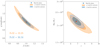 |
Fig. 1. Confidence areas of the scale parameter f and amplitude parameter g (left panel) and the confidence areas of the halo mass Mh and halo concentration c jointly derived from the constraints on the f and g parameters (right panel) for an analysis of the mock KiDS+GAMA area. Orange contours show the maximum likelihood fit on the stacked tangential shear profiles, and the blue contours the maximum likelihood fit as it was performed on the ellipticities of sources used directly, using all the galaxies in the mock field simultaneously. Shown are the best-fitting values for each method (orange and blue crosses) and the fiducial lens model (red circle). The contours correspond to the case with 50 lenses per deg2 in the simulated field. |
Best-fit values.
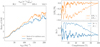 |
Fig. 2. Left panel: figure of merit as a function of lens number density in a simulated 1 deg2 field. The orange line shows the case where we consider all the galaxies in the field, and thus gives us an estimate of improvement in precision when using a two-dimensional method. The improvement levels off at a value of around 5, which indicates that in dense galaxy fields, the loss of signal-to-noise ratio due to the limited number of sources cannot be overcome. The blue line shows the case where we apply a typical KiDS survey mask to our mock catalogues. Right panel: relative shift of the halo mass Mh (top) and halo concentration c (bottom) derived from the constraints on the f and g parameters from the fiducial model as a function of completeness. Shown are the shift of the recovered parameters for the one-dimensional method (solid lines) and the shift of the recovered parameters for the two-dimensional method (dashed lines). Also shown is a typical completeness due to a mask in a KiDS like survey (vertical grey line). |
We now focus on the second question in our investigation, whether there is any bias introduced when not all lensing galaxies are accounted for. To this end, we use the same KiDS-like mock field with 720 lens galaxies, but now we remove one lens in each iteration, thus effectively accounting for the possible bias we might introduce in real observations by not accounting for galaxies just outside of our observed field or not accounting for lens galaxies that were masked out of the data. Figure 2 shows the shift of the best-fit parameters away from the fiducial model as a function of the field completeness, averaged over five different realisations of the lens distribution. What is immediately clear is that the NFW fit to the one-dimensional tangential shear profiles recovers the true input parameters (as it is essentially removing any configuration information from the sample by the tangential averaging), also for the cases of low completeness. The two-dimensional method can only do this successfully at high completeness values; any small deviation and unexpected features in the field caused by the presence of lenses not accounted for drives the recovered values of the input parameters away from the truth as the model tries to accommodate the missing lenses.
We also study the effect of the masking introduced by a realistic KiDS survey mask, shown in Fig. 3. We apply this mask to our mock catalogues and repeat the fitting of our model to the lenses and sources that remain in the mock catalogues. We again change the number of lenses in the field and the results of this exercise can be seen in Fig. 2 (blue line). What can be observed is that the two-dimensional method, even in the case of masking, is still more precise, and that the difference in precision is a direct result of the amount of masked area. The accuracy of the method due to masking behaves in a similar way to that shown in Fig. 2, but the observed bias is smaller because a larger number of lenses remain in the field. A typical KiDS survey mask reduces the number of lenses by about 20% (Kuijken et al. 2015; de Jong et al. 2015; Hildebrandt et al. 2017), which can bias the fitted parameters up to 10%, as shown in Fig. 2 (vertical grey line). This needs to be accounted for in an application to real data.
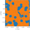 |
Fig. 3. Typical KiDS survey r-band mask used to evaluate the effect of masking on the inference of best-fit parameters, and the possible bias masking might introduce. |
Thus far we have ignored systematic biases in the galaxy shape measurements. They can be split into a multiplicative bias, which leads to an overall scaling of the signal, and an additive bias that manifests as a preferred orientation of galaxies. As the former simply scales the signal, the impact on the one-dimensional and two-dimensional analyses is the same. The situation is different in the case of additive bias: a constant signal will simply vanish when we consider the azimuthally averaged tangential shear (in the limit of no edge effects). Even a spatially varying additive bias is expected to vanish because it typically does not align with the line connecting the lens and the source. In contrast, in the two-dimensional case we expect the χ2 to become poor as the systematic signal contributes to it. To examine whether this has any impact on the recovered model parameters we mimic a systematic shape measurement error by adding a constant uniform shear to our mock dataset and repeat our analysis. We find that the overall χ2 surface indeed becomes offset by a constant (positive) value; however, we are nonetheless able to recover the input parameters exactly as in our fiducial case2.
5. Evaluation of the two methods with the EAGLE simulation
Motivated by the success of the two-dimensional galaxy–galaxy lensing method from the previous section, we now focus on more realistic tests using the EAGLE hydrodynamical simulation (Schaye et al. 2015; Crain et al. 2015; McAlpine et al. 2016) as our input data. Studying a simulation gives us the ability to compare our two-dimensional galaxy–galaxy lensing results against the truth, properties as measured directly from particle properties in the simulation. We note that for the purpose of this study we do not use a lightcone generated from the EAGLE simulation. Although we include complexities of neighbouring galaxies, we do not capture projections along the line of sight or missing galaxies, for example. We use the AGN simulation AGNdT9L0050N0752, which has 7523 dark matter particles and a box size of 50 comoving Mpc (Schaye et al. 2015), and it is calibrated in such a way that it reproduces global observables of our Universe. The EAGLE simulation was also shown to correctly predict the galaxy–galaxy lensing signal when compared to the KiDS+GAMA data (Velliscig et al. 2017), for both central and satellite galaxies. We take the full particle information in a box with a comoving size of 50 Mpc which is then binned to 8195 × 8195 × 8195 pixels. The box is then projected along the axes, yielding three different mass maps of the EAGLE simulation. To calculate the shear at each location, we first position the mass map at redshift of 0.2 (by scaling it comovingly), calculate the density map using the mean density of the Universe, and use the Kaiser & Squires (1993) prescription to calculate the shear, rolling the edges of the map. Because we want the sources to be positioned at a redshift that resembles the typical source redshift in the KiDS survey, we calculate the convergence map using the critical surface mass density at redshift of 0.7. A small portion of an EAGLE shear map is shown in Fig. 4. The whole EAGLE map corresponds to a 60 deg2 patch of sky.
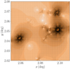 |
Fig. 4. Segment of the shear map derived from the EAGLE particle data. A number of notable features of weak lensing are visible in this plot. The ellipticites are tangentially aligned with the lenses and the strength of gravitational lensing diminishes with distance from the lens. The lens configuration creates a unique pattern that contains information about mass distribution that is otherwise lost when tangentially averaging the observed shears. |
Further information about the properties of the lens galaxies are queried from the public EAGLE database (McAlpine et al. 2016), such as the total halo mass, centre of mass, centre of potential, stellar mass, stellar mass within certain aperture, group memberships, and group properties. From the database we select galaxies with stellar masses ranging from 109.6 M⊙ to 1011.2 M⊙, which is a range that allows us to have enough galaxies in finer stellar mass bins (which we will use for our fiducial stacked tangential shear method) and ensures that the galaxies in EAGLE are well defined in terms of simulation particle mass. From this selection of galaxies we take both the centrals and satellite galaxies. Inclusion of satellite galaxies in the study is crucial for the two-dimensional method, as otherwise the results can be substantially biased (up to 10% for typical survey masks), as demonstrated in the previous section and in Fig. 2, and at the same time it allows their properties to be studied, as was previously done using the one-dimensional method, by Sifón et al. (2015), amongst others. In total, after applying all the selection criteria, we are left with 859 galaxies (520 centrals and 339 satellites).
We calculate the tangential shear signal for each galaxy in our sample using the tangential ϵt component of the source’s ellipticity around the position of the lens. The azimuthal average of the tangential ellipticity is then our unbiased estimate of the tangential shear. For the two-dimensional method, we use the ϵ1 and ϵ2 values directly. The tangential shear profiles and their averages for the 1010.8–1011.0 M⊙ stellar mass bin can be seen in Fig. 6. The noisiness of the individual profiles can be directly attributed to the fact that we are azimuthally averaging the data on a square grid.
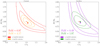 |
Fig. 7. Left panel: confidence areas of the halo mass Mh and concentration c of central galaxies for the analysis of the EAGLE simulation using the one-dimensional method and the two-dimensional method, scaled with the input stellar-to-halo mass relation and the concentration–mass relation. Right panel: confidence areas of the halo mass Mh and concentration c of satellite galaxies for the analysis of the EAGLE simulation using the one-dimensional method and the two-dimensional method, scaled with the input stellar-to-halo mass relation and the concentration–mass relation. The contours show the results of the maximum likelihood fit on the central galaxies (red and purple) and satellite galaxies (orange and green). Crosses (in corresponding colours) show the best-fitting values for each method and galaxy sample, and the red circles show the fiducial models. The contours are calculated from the contours obtained as a fit of the f and g parameters. |
The central and satellite galaxies in the EAGLE simulation follow a different stellar-to-halo mass relation, and we also account for this in the model. For this we use the same relation used in Sect. 3 and we fit it to the halo masses derived from the NFW fits to the convergence field of individual galaxies, both centrals and satellites (this is done in order to use the same definition of the halo mass for both galaxy types). The two stellar-to-halo mass relations are shown in Fig. 5, and the parameters obtained are listed in Table 2. The different stellar-to-halo mass relations are then accounted for in the modified lens model that differentiates between the central and satellite galaxies for the one-dimensional method and for the two-dimensional method. From the same fit we note that the concentrations of the haloes are generally lower than the prediction from Duffy et al. (2008). While they still follow the same trend, the normalisation of the relation is lower for both centrals and satellites, with a normalisation of 0.6 for centrals and 0.25 for satellites, with the lower values arising because we include all the haloes, not only the relaxed ones. This is consistent with what was found by Viola et al. (2015).
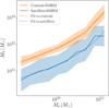 |
Fig. 5. Stellar-to-halo mass relation for the central galaxies in the EAGLE simulation (in orange) and for the satellites (in blue). Shown are the median stellar-to-halo mass relation (solid lines) with the corresponding scatter (filled areas). The dashed lines are the models for the stellar-to-halo mass relation used in the analysis. |
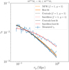 |
Fig. 6. Stacked tangential shear profiles for the lenses selected from the EAGLE simulation (blue lines) in the 1010.8 to 1011.0 M⊙ stellar mass bin. The dashed orange, red, and black lines show the signals predicted by our fiducial lens model using f = 1 and g = 1 for NFW, satellites, and centrals, respectively. The total best-fitting model is shown with the solid orange line and the best-fitting model for centrals and satellites in solid black and red lines, respectively. The corresponding halo masses and concentrations of input models and the best-fit results are listed in Table 3. |
Parameters of the stellar-to-halo mass relation.
Central values of the input and best-fit halo masses and concentrations.
We fit the two lens models3 to the mean tangential shear profiles per bin and to the full ellipticity data using Eqs. (5) and (7). To account for the uncertainty in our ellipticity measurements we again assign the standard deviation of 0.3, scaled to the typical number density of GAMA and KiDS set-up due to the size of the pixel in our mass maps. This results in an uncertainty of σϵ = 0.015. The gain in precision is 3.9, which is the ratio of the area of the 68% confidence level contours (FoM2D/FoM1D = 3.9). We show the separate credibility contours for the halo mass and concentration in Fig. 7 for the one-dimensional and two-dimensional methods, separated into contributions from central and satellite galaxies; both values are scaled with the input stellar-to-halo mass relation and the concentration–mass relation, which then show the relative change of the halo masses and concentration from fiducial values obtained from the simulation.
At first sight it might seem that the results are somewhat biased with regard to the actual measured scaling relation of the EAGLE galaxies, but we do observe an almost equal effect on the f and g parameters for the two methods. This is not necessarily due to a bias in the analysis. After all, the intrinsic scatter in the concentration–mass relation and in the stellar mass-to-halo mass relation are not accounted for in the model and are the most likely cause of small shifts in the methods presented. Both methods also give robust estimates for the properties of central and satellite galaxies and given the results, the two-dimensional method is much more precise in constraining the two fitted parameters than the one-dimensional method. Given the large uncertainty on the recovered parameters of the one-dimensional method for satellite galaxies, the one-dimensional method is unable to robustly capture the contribution from satellites in the KiDS+GAMA data, as was also demonstrated by Sifón et al. (2015). Given the results of this exercise, we expect to capture the contribution from satellites when we apply the two-dimensional method to the data.
6. Discussion and conclusions
We have investigated the precision and bias of one and two-dimensional galaxy–galaxy lensing analyses of weak lensing data, using tangential averaged shear profiles and ellipticities, respectively, keeping in mind current and upcoming state-of-the-art large weak lensing galaxy surveys. The main difference between the two methods lies in the fact that the two-dimensional approach uses all the available information in an observed field. While the one-dimensional method uses only the ellipticities of source galaxies to infer the stacked tangential shear signal, the two-dimensional method uses actual relative positions of all the lens galaxies in a field and the ellipticities of all the sources in the field. Because the two-dimensional galaxy–galaxy lensing accounts for spatial configuration of the lens galaxies, the unique signatures in the shear field caused by overlapping regions of influence contain more information about the halo properties of the lenses we want to study and result in a significant improvement over the traditional one-dimensional stacking methods.
We tested the method on mock observations generated in a semi-empirical way where we assumed a model with the gravitational lenses represented by the NFW profiles with properties determined from observable quantities such as stellar mass, taking into account a typical configuration and properties of KiDS and GAMA surveys. We find that the two-dimensional method gives better constraints on those same parameters: the FoM is more than three times larger compared to the results from stacked tangential shear profiles. This suggests that there can be an equal amount of information hidden in the exact configuration of the lenses and their overlaps, which is lost when a one-dimensional method is used. The precision gain also depends on the lens density. In denser fields of gravitational lenses, the gain in precision from using the two-dimensional method is larger, as the signal becomes more heavily influenced by neighbouring gravitational lenses. We also studied the case where we removed a significant fraction of galaxies present in a mock field from our analysis, and while the two-dimensional method still gives us better constraints on the NFW parameters, the accuracy of these parameters starts to suffer because the modelling of the lenses does not account for the contributions of shears that are caused by the galaxies we left out of our analysis. While this indeed produces a noticeable bias, and thus needs to be corrected to properly recover the true values of the parameters we study, the case where such a large fraction of galaxies would be missed is rather severe. This effect of correlated structure – undetected galaxies that are clustered with the observed galaxies and the matter distribution on group scale – is in reality negligibly small (as discussed in detail already by Hudson et al. 1998).
We assumed a model where lenses are represented by the NFW profiles, up to constant pre-factors for the lensing signal amplitude and scale. We used the same lens model as well for the study on the EAGLE simulation (Schaye et al. 2015; McAlpine et al. 2016). As we used the concentration–mass relation that closely describes the one measured in the EAGLE simulation and a stellar-to-halo mass relation of the EAGLE central and satellite galaxies in our lens model, we expected both methods to recover the input parameters values. We find that the two methods are able to almost perfectly recover these values, and the small differences can be attributed to the non-ideal modelling of the galaxies in the EAGLE simulation. The two-dimensional method does indeed perform better.
Given that the two-dimensional galaxy–galaxy lensing method requires knowledge of group (and/or cluster) membership, preferentially inferred from spectroscopic data, we identify two cases where using the two-dimensional method could be preferred over the one-dimensional method. The most obvious one is studying the group properties as a function of halo mass, where using the two-dimensional method can give better constraints on scaling relations of group halo mass with luminosity of central galaxies, their stellar mass, size, X-ray gas emission, and the concentration of such haloes. As we have precise membership information of galaxies in clusters and because of the increased number density of these galaxies, the second case is to study the sub-halo mass function of galaxy clusters to a high precision. The two-dimensional galaxy–galaxy lensing, together with the group or cluster membership information that is available by using highly complete spectroscopic surveys is an obvious choice for galaxy–galaxy studies on dense galaxy fields in general.
We first calculate the γ(θ, zs) and the κ(θ, zs), then use Eq. (13) to calculate the reduced shear.
This can be explicitly seen by writing out the χ2 with the added constant shear, χ2 ∝ (γt + c − m)2, where c is the constant shear and m the model prediction. The cross terms in the expanded form average to 0 and we gain a constant term c2, which worsens the overall χ2, but does not inhibit the ability to minimise the (γt − m)2 difference.
One for centrals and one for satellites, for a combined set of four parameters; each model has a set of (f, g) parameters.
Acknowledgments
We thank the anonymous referee for the very useful comments and suggestions. We thank Mike Hudson for the useful discussion on the topic. AD acknowledges support from grant number 614.001.541 and HH acknowledges support from Vici grant number 639.043.512, both financed by the Netherlands Organisation for Scientific Research (NWO). KK acknowledges support from the Alexander von Humboldt Foundation. This work has made use of Python (http://www.python.org), including the packages numpy (http://www.numpy.org) and scipy (http://www.scipy.org). The plots were produced with matplotlib (Hunter 2007).
References
- Bartelmann, M., & Schneider, P. 2001, Phys. Rep., 340, 291 [NASA ADS] [CrossRef] [Google Scholar]
- Brouwer, M. M., Cacciato, M., Dvornik, A., et al. 2016, MNRAS, 462, 4451 [NASA ADS] [CrossRef] [Google Scholar]
- Brouwer, M. M., Visser, M. R., Dvornik, A., et al. 2017, MNRAS, 466, 2547 [NASA ADS] [CrossRef] [Google Scholar]
- Cacciato, M., van Uitert, E., & Hoekstra, H. 2014, MNRAS, 437, 377 [NASA ADS] [CrossRef] [Google Scholar]
- Cooray, A., & Sheth, R. 2002, Phys. Rep., 372, 1 [NASA ADS] [CrossRef] [Google Scholar]
- Courteau, S., Cappellari, M., De Jong, R. S., et al. 2014, Rev. Mod. Phys., 86, 47 [NASA ADS] [CrossRef] [Google Scholar]
- Crain, R. A., Schaye, J., Bower, R. G., et al. 2015, MNRAS, 450, 1937 [NASA ADS] [CrossRef] [Google Scholar]
- de Jong, J. T. A., Verdoes Kleijn, G. A., Boxhoorn, D. R., et al. 2015, A&A, 582, A62 [NASA ADS] [CrossRef] [EDP Sciences] [Google Scholar]
- Driver, S. P., Hill, D. T., Kelvin, L. S., et al. 2011, MNRAS, 413, 971 [NASA ADS] [CrossRef] [Google Scholar]
- Duffy, A. R., Schaye, J., Kay, S. T., & Dalla Vecchia, C. 2008, MNRAS, 390, L64 [NASA ADS] [CrossRef] [Google Scholar]
- Dvornik, A., Hoekstra, H., Kuijken, K., et al. 2018, MNRAS, 479, 1240 [NASA ADS] [CrossRef] [Google Scholar]
- Geiger, B., & Schneider, P. 1999, MNRAS, 302, 118 [NASA ADS] [CrossRef] [Google Scholar]
- Han, J., Eke, V. R., Frenk, C. S., et al. 2015, MNRAS, 446, 1356 [NASA ADS] [CrossRef] [Google Scholar]
- Hildebrandt, H., Viola, M., Heymans, C., et al. 2017, MNRAS, 465, 1454 [Google Scholar]
- Hoekstra, H. 2003, MNRAS, 339, 1155 [NASA ADS] [CrossRef] [Google Scholar]
- Hoekstra, H. 2014, Proc. Int. Sch. Phys. Enrico Fermi, 186, 59 [Google Scholar]
- Hoekstra, H., Franx, M., Kuijken, K., Carlberg, R. G., & Yee, H. K. C. 2003, MNRAS, 340, 609 [NASA ADS] [CrossRef] [Google Scholar]
- Hoekstra, H., Yee, H. K. C., & Gladders, M. D. 2004, ApJ, 606, 67 [NASA ADS] [CrossRef] [Google Scholar]
- Hudson, M. J., Gwyn, S. D. J., Dahle, H., & Kaiser, N. 1998, ApJ, 503, 531 [NASA ADS] [CrossRef] [Google Scholar]
- Hunter, J. D. 2007, Comput. Sci. Eng., 9, 90 [NASA ADS] [CrossRef] [Google Scholar]
- Kaiser, N., & Squires, G. 1993, ApJ, 404, 441 [NASA ADS] [CrossRef] [Google Scholar]
- Kuijken, K., Heymans, C., Hildebrandt, H., et al. 2015, MNRAS, 454, 3500 [NASA ADS] [CrossRef] [Google Scholar]
- Leauthaud, A., Tinker, J., Behroozi, P. S., Busha, M. T., & Wechsler, R. H. 2011, ApJ, 738, 45 [NASA ADS] [CrossRef] [Google Scholar]
- Liske, J., Baldry, I. K., Driver, S. P., et al. 2015, MNRAS, 452, 2087 [NASA ADS] [CrossRef] [Google Scholar]
- Matthee, J., Schaye, J., Crain, R. A., et al. 2017, MNRAS, 465, 2381 [NASA ADS] [CrossRef] [Google Scholar]
- McAlpine, S., Helly, J., Schaller, M., et al. 2016, Astron. Comput., 15, 72 [NASA ADS] [CrossRef] [Google Scholar]
- McKay, M., Beckman, R., & Canover, W. 1979, Technometrics, 21, 239 [Google Scholar]
- Navarro, J. F., Frenk, C. S., & White, S. D. M. 1996, ApJ, 462, 563 [NASA ADS] [CrossRef] [Google Scholar]
- Peacock, J. A., & Smith, R. E. 2000, MNRAS, 318, 1144 [NASA ADS] [CrossRef] [Google Scholar]
- Planck Collaboration XVI. 2014, A&A, 571, A16 [NASA ADS] [CrossRef] [EDP Sciences] [Google Scholar]
- Robotham, A. S. G., Norberg, P., Driver, S. P., et al. 2011, MNRAS, 416, 2640 [NASA ADS] [CrossRef] [Google Scholar]
- Schaller, M., Frenk, C. S., Bower, R. G., et al. 2015, MNRAS, 451, 1247 [NASA ADS] [CrossRef] [Google Scholar]
- Schaye, J., Crain, R. A., Bower, R. G., et al. 2015, MNRAS, 446, 521 [Google Scholar]
- Schneider, P. 2003, ArXiv e-prints [arXiv: astro-ph/0306465] [Google Scholar]
- Schneider, P., & Rix, H.-W. 1997, ApJ, 474, 25 [NASA ADS] [CrossRef] [Google Scholar]
- Seljak, U. 2000, MNRAS, 318, 203 [NASA ADS] [CrossRef] [Google Scholar]
- Sifón, C., Cacciato, M., Hoekstra, H., et al. 2015, MNRAS, 454, 3938 [NASA ADS] [CrossRef] [Google Scholar]
- Sonnenfeld, A., & Leauthaud, A. 2018, MNRAS, 477, 5460 [NASA ADS] [CrossRef] [Google Scholar]
- van Uitert, E., Hoekstra, H., Velander, M., et al. 2011, A&A, 534, A14 [NASA ADS] [CrossRef] [EDP Sciences] [Google Scholar]
- van Uitert, E., Cacciato, M., Hoekstra, H., et al. 2016, MNRAS, 459, 3251 [NASA ADS] [CrossRef] [Google Scholar]
- Velander, M., van Uitert, E., Hoekstra, H., et al. 2014, MNRAS, 437, 2111 [NASA ADS] [CrossRef] [Google Scholar]
- Velliscig, M., Cacciato, M., Hoekstra, H., et al. 2017, MNRAS, 471, 2856 [NASA ADS] [CrossRef] [Google Scholar]
- Viola, M., Cacciato, M., Brouwer, M., et al. 2015, MNRAS, 452, 3529 [CrossRef] [Google Scholar]
- Wright, C. O., & Brainerd, T. G. 2000, ApJ, 534, 34 [NASA ADS] [CrossRef] [Google Scholar]
All Tables
All Figures
|
Fig. 1. Confidence areas of the scale parameter f and amplitude parameter g (left panel) and the confidence areas of the halo mass Mh and halo concentration c jointly derived from the constraints on the f and g parameters (right panel) for an analysis of the mock KiDS+GAMA area. Orange contours show the maximum likelihood fit on the stacked tangential shear profiles, and the blue contours the maximum likelihood fit as it was performed on the ellipticities of sources used directly, using all the galaxies in the mock field simultaneously. Shown are the best-fitting values for each method (orange and blue crosses) and the fiducial lens model (red circle). The contours correspond to the case with 50 lenses per deg2 in the simulated field. |
| In the text | |
|
Fig. 2. Left panel: figure of merit as a function of lens number density in a simulated 1 deg2 field. The orange line shows the case where we consider all the galaxies in the field, and thus gives us an estimate of improvement in precision when using a two-dimensional method. The improvement levels off at a value of around 5, which indicates that in dense galaxy fields, the loss of signal-to-noise ratio due to the limited number of sources cannot be overcome. The blue line shows the case where we apply a typical KiDS survey mask to our mock catalogues. Right panel: relative shift of the halo mass Mh (top) and halo concentration c (bottom) derived from the constraints on the f and g parameters from the fiducial model as a function of completeness. Shown are the shift of the recovered parameters for the one-dimensional method (solid lines) and the shift of the recovered parameters for the two-dimensional method (dashed lines). Also shown is a typical completeness due to a mask in a KiDS like survey (vertical grey line). |
| In the text | |
|
Fig. 3. Typical KiDS survey r-band mask used to evaluate the effect of masking on the inference of best-fit parameters, and the possible bias masking might introduce. |
| In the text | |
|
Fig. 4. Segment of the shear map derived from the EAGLE particle data. A number of notable features of weak lensing are visible in this plot. The ellipticites are tangentially aligned with the lenses and the strength of gravitational lensing diminishes with distance from the lens. The lens configuration creates a unique pattern that contains information about mass distribution that is otherwise lost when tangentially averaging the observed shears. |
| In the text | |
|
Fig. 7. Left panel: confidence areas of the halo mass Mh and concentration c of central galaxies for the analysis of the EAGLE simulation using the one-dimensional method and the two-dimensional method, scaled with the input stellar-to-halo mass relation and the concentration–mass relation. Right panel: confidence areas of the halo mass Mh and concentration c of satellite galaxies for the analysis of the EAGLE simulation using the one-dimensional method and the two-dimensional method, scaled with the input stellar-to-halo mass relation and the concentration–mass relation. The contours show the results of the maximum likelihood fit on the central galaxies (red and purple) and satellite galaxies (orange and green). Crosses (in corresponding colours) show the best-fitting values for each method and galaxy sample, and the red circles show the fiducial models. The contours are calculated from the contours obtained as a fit of the f and g parameters. |
| In the text | |
|
Fig. 5. Stellar-to-halo mass relation for the central galaxies in the EAGLE simulation (in orange) and for the satellites (in blue). Shown are the median stellar-to-halo mass relation (solid lines) with the corresponding scatter (filled areas). The dashed lines are the models for the stellar-to-halo mass relation used in the analysis. |
| In the text | |
|
Fig. 6. Stacked tangential shear profiles for the lenses selected from the EAGLE simulation (blue lines) in the 1010.8 to 1011.0 M⊙ stellar mass bin. The dashed orange, red, and black lines show the signals predicted by our fiducial lens model using f = 1 and g = 1 for NFW, satellites, and centrals, respectively. The total best-fitting model is shown with the solid orange line and the best-fitting model for centrals and satellites in solid black and red lines, respectively. The corresponding halo masses and concentrations of input models and the best-fit results are listed in Table 3. |
| In the text | |
Current usage metrics show cumulative count of Article Views (full-text article views including HTML views, PDF and ePub downloads, according to the available data) and Abstracts Views on Vision4Press platform.
Data correspond to usage on the plateform after 2015. The current usage metrics is available 48-96 hours after online publication and is updated daily on week days.
Initial download of the metrics may take a while.