| Issue |
A&A
Volume 627, July 2019
|
|
|---|---|---|
| Article Number | A165 | |
| Number of page(s) | 26 | |
| Section | Planets and planetary systems | |
| DOI | https://doi.org/10.1051/0004-6361/201935089 | |
| Published online | 18 July 2019 | |
A spectral survey of an ultra-hot Jupiter
Detection of metals in the transmission spectrum of KELT-9 b★
1
Observatoire de Genève, University of Geneva, Chemin des Maillettes, 1290 Sauverny,
Switzerland
e-mail: This email address is being protected from spambots. You need JavaScript enabled to view it.
2
Center for Space and Habitability, Universität Bern,
Gesellschaftsstrasse 6, 3012 Bern,
Switzerland
e-mail: This email address is being protected from spambots. You need JavaScript enabled to view it.
3
Leiden Observatory, Universiteit Leiden,
Niels Bohrweg 2, 2333 CA Leiden,
The Netherlands
4
Anton Pannekoek Institute of Astronomy, University of Amsterdam,
Science Park 904,
1098 XH Amsterdam,
The Netherlands
5
Cavendish Astrophysics Battcock Centre for Experimental Astrophysics, Cavendish Laboratory, Cambridge University, JJ Thomson Avenue, CB3 0HE Cambridge,
UK
6
MRC Laboratory of Molecular Biology, Francis Crick Avenue, Cambridge Biomedical Campus, Cambridge University, CB2 0QH Cambridge,
UK
7
Zentrum für Astronomie und Astrophysik, Technische Universität Berlin,
Hardenbergstrasse 36,
10623 Berlin,
Germany
8
Department of Chemistry and Environmental Science, Medgar Evers College, City University of New York, 1650 Bedford Avenue, Brooklyn, NY 11235,
USA
Received:
18
January
2019
Accepted:
3
May
2019
Abstract
Context. KELT-9 b exemplifies a newly emerging class of short-period gaseous exoplanets that tend to orbit hot, early type stars – termed ultra-hot Jupiters. The severe stellar irradiation heats their atmospheres to temperatures of ~4000 K, similar to temperatures of photospheres of dwarf stars. Due to the absence of aerosols and complex molecular chemistry at such temperatures, these planets offer the potential of detailed chemical characterization through transit and day-side spectroscopy. Detailed studies of their chemical inventories may provide crucial constraints on their formation process(es) and evolution history.
Aims. We aim to search the optical transmission spectrum of KELT-9 b for absorption lines by metals using the cross-correlation technique.
Methods. We analysed two transit observations obtained with the HARPS-N spectrograph. We used an isothermal equilibrium chemistry model to predict the transmission spectrum for each of the neutral and singly ionized atoms with atomic numbers between three and 78. Of these, we identified the elements that are expected to have spectral lines in the visible wavelength range and used those as cross-correlation templates.
Results. We detect (>5σ) absorption by Na I, Cr II, Sc II and Y II, and confirm previous detections of Mg I, Fe I, Fe II, and Ti II. In addition, we find evidence of Ca I, Cr I, Co I, and Sr II that will require further observations to verify. The detected absorption lines are significantly deeper than predicted by our model, suggesting that the material is transported to higher altitudes where the density is enhanced compared to a hydrostatic profile, and that the material is part of an extended or outflowing envelope. There appears to be no significant blue-shift of the absorption spectrum due to a net day-to-night side wind. In particular, the strong Fe II feature is shifted by 0.18 ± 0.27 km s−1, consistent with zero. Using the orbital velocity of the planet we derive revised masses and radii of the star and the planet: M* = 1.978 ± 0.023 M⊙, R* = 2.178 ± 0.011 R⊙, mp = 2.44 ± 0.70 MJ and Rp = 1.783 ± 0.009 RJ.
Key words: planets and satellites: gaseous planets / techniques: spectroscopic
Cross-correlation templates are available at the CDS via anonymous ftp to cdsarc.u-strasbg.fr (130.79.128.5) or via http://cdsarc.u-strasbg.fr/viz-bin/qcat?J/A+A/627/A165
CHEOPS Fellow.
© ESO 2019
1 Introduction
Hot Jupiters provide a unique window into the nature of the exoplanet population due to the combination of their size, high temperature and short orbital periodicity. Furthermore, their atmospheres are often inflated (Baraffe et al. 2010), making them especially amenable for transmission spectroscopy during transit events. During a transit some starlight passes through the upper atmosphere of the planet, where certain wavelengths are absorbed depending on its chemical composition. This wave- length-dependent absorption manifests itself as a wavelength-dependence of the apparent radius of the planet. The spectrum of the atmosphere generally has two components: line-absorption caused by discrete energy transitions in atoms and molecules, and continuum absorption or scattering caused by molecules or aerosol particles.
The identification and measurement of the relative strengths of spectral lines and bands in the transmission spectra of exoplanets have been used to put constraints on the atmospheric composition and thermal structure (see e.g. Vidal-Madjar et al. 2003; Redfield et al. 2008; Sing et al. 2008; Huitson et al. 2012; Wyttenbach et al. 2015; Nikolov et al. 2018; Spake et al. 2018), with the ultimate aim of providing constraints on their formation scenario and evolution (Madhusudhan et al. 2014; Kreidberg et al. 2015; Mordasini et al. 2016; Brewer et al. 2017). In addition, these lines may be used to probe atmospheric dynamics because velocity streams in the atmosphere cause the spectral lines to be Doppler-shifted away from the rest-frame velocity of the planet (Snellen et al. 2010; Miller-Ricci Kempton & Rauscher 2012; Showman et al. 2013; Kempton et al. 2014; Louden & Wheatley 2015; Brogi et al. 2016; Allart et al. 2018).
Access to the information contained in individual absorption lines requires high spectral resolution in the order of  . Such spectral resolution is generally limited to ground-based instrumentation, mostly in the form of optical and NIR echelle spectrographs. When seen in transmission, the spectral lines formed in the lower part of the atmosphere of a typical hot Jupiter can have depths of up to ~ 10−3 times the flux of the host star. To reach this sensitivity with high-resolution spectrographs on present-day telescopes, many targeted absorption lines can be combined using a form of cross-correlation. Besides raising the sensitivity by averaging out the photon noise, the use of cross-correlation has the advantage of providing additional robustness against spurious spectral features, because the distribution of absorption lines is unique for each species, and follows the radial velocity of the planet (Snellen et al. 2010; Brogi et al. 2012). As such, enhancements of the cross-correlation function arehard to mimic by systematic noise that is not correlated with the absorption line spectrum of the target species.
A theoretical study by Kitzmann et al. (2018) predicted the presence of absorption lines of iron (Fe) in the transmission spectrum of the ultra-hot Jupiter KELT-9 b. KELT-9 b orbits the bright A0 star HD 195689 with a periodicity of 1.48 days (Gaudi et al. 2017). Due to its close orbital distance of approximately 0.03 AU (Gaudi et al. 2017), it is heated to an equilibrium temperature of 4050 ± 180 K, similar to the photospheres of many dwarf stars. Such temperatures are high enough to justify simplifying assumptions of equilibrium chemistry and a nearly purely atomic gas at the dayside and terminator regions (Arcangeli et al. 2018; Kitzmann et al. 2018; Lothringer et al. 2018; Parmentier et al. 2018). Potentially, this greatly simplifies the interpretation of the transmission spectrum of KELT-9 b when compared to other hot Jupiters for which aerosols and non-equilibrium chemistry are important factors. However, the night-side of the planet is expected to be in a much cooler regime that is likely characterized by complex molecular chemistry and condensation. Condensed droplets and grains may rain out to the interior of the planet, potentially depleting these species from the atmosphere in what is known as a cold-trap (Spiegel et al. 2009). Depending on the circulation efficiency, these species may then be transported back to the hot day side where they can again evaporate into the gas phase and dissociate to produce atomic absorption lines that can be observed in the transmission spectrum (Showman et al. 2009; Fortney et al. 2010). The observed transmission spectrum is therefore expected to be linked to the chemistry elsewhere on the planet via the global circulation pattern. Regardless, chemical equilibrium is a valid assumption on the hot day-side and terminator region due to the efficiency of thermal reactions at these high temperatures, given the elementary abundances at these locations as set by global circulation processes (Kitzmann et al. 2018). Seeking to validate the predictions by Kitzmann et al. (2018) we previously applied the cross-correlation technique to transit observations obtained with the high-resolution HARPS-North (HARPS-N) spectograph and found the presence of absorption lines by neutral iron (Fe I), but also strong lines of ionized iron (Fe II) and titanium (Ti II) (Hoeijmakers et al. 2018a). In addition, Balmer lines of hydrogen where observed by Yan & Henning (2018) and Cauley et al. (2019) in the transmission spectrum of the same planet, as well as individual lines of Fe I, Fe II and the Mg I triplet (Cauley et al. 2019).
In July of 2018 we obtained a second transit observation with the HARPS-N spectrograph and proceeded to perform a survey for additional species that have absorption lines in the optical range of HARPS-N, using the high-resolution cross-correlation technique. This survey includes all neutral and singly ionized species with atomic numbers three to 78 (lithium to platinum)1 for which adequate line-list data is available. This paper proceeds to describe the observations and the analysis method in Sect. 2 (with a detailed description of our application of the cross-correlation operation in Appendix A), the cross-correlation templates in Sect. 3 and the results of the survey in Sect. 4.
Overview of the observations with HARPS-N.
2 Observations and cross-correlation analysis
We have observed two transits with the HARPS-North spectrograph mounted on the 3.58-m Telescopio Nazionale Galileo (TNG) in La Palma, Spain, on 31-07-2017 (programme A35DDT4, hereafter Night 1) and on 20-07-2018 (programme OPT18A-38, hereafter Night 2). Both programmes have been carried out in the frame work of the “Sensing Planetary Atmospheres with Differential Echelle Spectroscopy” (SPADES) survey. Results from Night 1 have been previously published in Hoeijmakers et al. (2018a).
HARPS-North is an optical spectrograph that covers wavelengths between 387.4 and 690.9 nm at a spectral resolution of R ~ 115 000, corresponding to a Doppler velocity of ~ 2.7 km s−1. The observations were obtained during both 3.9-h transits, as well as during 5.0 and 4.5 h baseline before and after the transit events. The exposure time was fixed to 600 s, yielding runs of 49 and 46 exposures, 19 of which took place during either transit (see Table 1). The observations of the second night were affected by a loss of flux in the bluest orders caused by an error in the control software of the Atmospheric Dispersion Corrector (ADC). Figure 1 shows the average one-dimensional spectrum of the KELT-9 system as observed by HARPS-N.
The raw spectra were reduced using the HARPS Data Reduction Software (DRS, version 3.8) which interpolates the extracted spectra on a uniform grid with a spacing of 0.01 Å. Absorption lines of the Earth atmosphere (telluric contamination) were corrected for using the MOLECFIT package (Smette et al. 2015) following Allart et al. (2017), and the subsequent analysis followed the general procedure from previous studies that use the high-resolution cross-correlation technique (e.g. Snellen et al. 2010; Brogi et al. 2012), in particular the analyses used in Hoeijmakers et al. (2018a) for the data of Night 1, and Hoeijmakers et al. (2018b).
For reasons of computational efficiency, we sub-divided the one-dimensional spectra in 15 sections of 20 nm width (each containing 20 000 spectral pixels)2, and performed the following analysis on each section individually. To isolate the signature of the planet, each spectrum was normalized to its median value and divided through the mean of the out-of-transit spectra, F(λ, tout). We then constructed an outlier-mask by flattening each spectrum using a median filter (to remove broadband continuum variations) followed by applying a running standard deviation, both with a width (in wavelength) of 75 pixels. All values that were more than 5σ away were flagged as NaNs and the previous normalization and removal of the mean out-of-transit spectrum were repeated. The resulting residuals were then filtered using a Gaussian high-pass filter with a 1σ width of 75 pixels, and any remaining 5σ outliers were again flagged and added to the outlier mask. This amounted to a total of 1729 and 8712 spectral pixels in nights 1 and 2 respectively.In addition, we masked out selected regions with systematic residuals inside strong telluric absorption lines (notably residuals caused by the O2 bands) and regions with low signal-to-noise. In this way 23 226 and 72 542 pixels were removed additionally. In total, 0.38% of all spectral pixels were masked out.
This procedure effectively yields the transmission spectrum  , as the ratio between each spectrum obtained at time t divided by the average out-of-transit spectrum.
The cross-correlation, c, is performed using a weighted mask (template), T, that acts to co-add the individual spectral pixels in the transmission spectrum observed at time, t, for velocity shifts between ± 1000 km s−1 in steps of 2 km s−1. This procedure follows the practise of Baranne et al. (1996), Pepe et al. (2002), Allart et al. (2017) a.o. and is prescribed in Eq. (1):
 (1)
(1)
Here xi(t) are each of the N spectral points in the transmission spectrum obtained at time t, Ti (v) are the corresponding values of the template that is Doppler shifted to a radial velocity, v. T takes on non-zero values inside a spectral line of interest, and zero in the continuum. Furthermore, T is normalized such that  . This operation thus effectively computes a weighted average of the absorption in the transmission spectrum at the location of the spectral lines included in the template. Because c(v, t) is computed for each 20 nm bin and each exposure of the time-series, we co-add these into a one-dimensional measurement of the average line profile in-transit. This average is weighted for the signal-to-noise ratio (S/N) obtained in each exposure, in each spectral bin,as detailed in Appendix A. This procedure is consistent with the approach applied in Hoeijmakers et al. (2018a).
We follow Hoeijmakers et al. (2018a) in producing an empirical model of the Doppler shadow that is caused by the obscuration of only part of the stellar absorption lines, effectively deforming them during the planetary transit (see Fig. 2). We characterize the shadow by cross-correlating the data with a continuum-normalized PHOENIX model of the stellar photosphere corresponding to an effective temperature of 10 000 K, log(g) = 4.5 and solar metallicity (Husser et al. 2013). The resulting cross-correlation profile is fit independently in each exposure using a Gaussian model. The resulting two-dimensional profile of c(v, t) is then modelled by fitting low-order polynomials through the obtained Gaussian fit parameters (centre position, amplitude and width), essentially requiring that the fit parameters of the Doppler shadow vary smoothly in time. Initially, this is only done for those exposures in which the signature of the Doppler shadow does not overlap with the signature of the atmosphere of the planet (the velocity of these overlap during part of the transit). This model is then subtracted, allowing the residual signature of the planet to bemodelled. The initial Doppler-shadow is fit again after subtracting the signature of the planet, this time including the region where the radial velocity of the planet and the Doppler shadow overlap. The same procedure is done for four additional signatures that may be associated with stellar pulsations, though these mostly occur at velocities that do not coincide with the velocity of the planet at any time during the transit (see Fig. 2).
The resulting two-dimensional model of the Doppler-shadow is subtracted from the cross-correlation profiles obtained for each of the various cross-correlation templates, multiplied by a scaling factor that minimizes the sum of the squared residuals – but ignoring cross-correlation values at which the planet signature is expected to be present. The values of these scaling factors are provided in Table C.1.
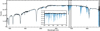 |
Fig. 1 Mean out-of-transit spectrum of the KELT-9 system as observed by HARPS-N, produced by stitching together the individual spectral orders after correction of the blaze function. The blue and black lines show the spectrum before and after telluric correction. The smaller panel shows the telluric water band that is highlighted in grey in detail, demonstrating the effect of the telluric correction. The outlying points are residuals of deep telluric absorption and a small number of emission lines that have remained uncorrected. |
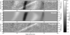 |
Fig. 2 Removal of the Doppler shadow for the first night of data. Top panel: two-dimensional cross-correlation function as obtained when using a PHOENIX 10 000 K stellar atmosphere model template. The dark feature near − 40 km s−1 is the Doppler shadow caused by the planet obscuring part of the disc-integrated stellar line, that is broadened by v sin i = 111.4 km s−1 (Gaudi et al. 2017). The bright linear slanted feature is the signature of the atmosphere of the planet. It appears in this cross-correlation because the star and the planet have ionized lines in common (Hoeijmakers et al. 2018a). It is ignored when constructing and fitting the model of the Doppler shadow. Besides these, there are significant cross-correlation residuals due to stellar line-shape variations that we tentatively attribute to pulsations of KELT-9 that are not characterized in the literature as of yet, but seem to resemble those that have been observed in hot δ Scuti stars such as β Pictoris (Koen et al. 2003) and Wasp-33 (Collier Cameron et al. 2010). Middle panel: full model as fit to this cross-correlation function, where the dashed line indicates the polynomial fit to the centroid velocities of the main shadow feature in each exposure. Bottom panel: residuals after removal. |
3 Cross-correlation templates
To compute the cross-correlation function, a mask is needed that defines the weights by which spectral pixels are co-added as per Eq. (1). We construct a mask for each species by forward modelling the transmission spectrum of KELT-9 b, assuming that it contains line-absorption of each species individually.
3.1 Opacity functions
Line-opacity functions are computed using HELIOS-K (Grimm & Heng 2015), adopting the transition tables from Kurucz (2018). As the partition functions in the database by Kurucz are not complete up to high atomic number, the partition functions were instead computed using the energy levels and statistical weights provided by the NISTdatabase when needed (Kramida et al. 2018a). Continuum opacity functions due to collision-induced absorption of H-He, H2 -H2 and H2-He were adopted from HITRAN (Richard et al. 2012), and H− bound–free and free–free absorption from John (1988). The Kurucz (2018) database includes broadening by radiation dampening, but not pressure broadening. This limitation does not significantly affect the analysis because the high-resolution transmission spectrum probes low pressures and the pressure-broadened wings are masked by the H− continuum which occurs at a pressure of around 3.5 mbar in these simulations (Kitzmann et al. 2018).
3.2 Chemistry
Chemistry calculations are done with the open source code FastChem (Stock et al. 2018). FastChem calculates the chemical equilibrium composition (i.e. assuming that all reaction rates are dominated by thermal timescales), and natively includes 560 chemical species. In addition, we add approximately 180 new ions to the set of species, that is, singly and doubly ionized atoms as well as some anions, for most elements lighter than neptunium (Z = 93). Because many of the required equilibrium constants are not available in the usual chemical databases (e.g. Chase et al. 1998), we calculate them using the Saha equation when needed (Saha 1920).
For the ionization reaction of, for example, caesium,
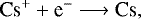 (2)
(2)
the corresponding temperature-dependent equilibrium constant for Cs+ is given by
 (3)
(3)
where n are the corresponding number densities of Cs, Cs+, and the free electrons, respectively.
To compute the right-hand side of Eq. (3) we employ the Saha equation, that describes the relation between the number densities n of two ionization levels i and i+ 1 at a given temperature,
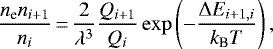 (4)
(4)
where λ is the thermal de Broglie wavelength of the electron, Q the corresponding partition function, and ΔE the energy difference between the two ionization levels. The partition functions are calculated based on the line transition database by Kurucz & Bell (1995) where available, and from those in the NIST Atomic Spectra Database (Kramida et al. 2018b), otherwise. The ionization energies are taken from the Lide (2004).
For doubly ionized species, the Saha equation is applied twice: once to evaluate the ratio
 (5)
(5)
and once more for the corresponding equation (Eq. (3)) for the number density of the singly ionized species. In the case of anions, ΔE in the Saha equation is replaced by the electron affinity.
The resulting mass action constants are fitted as a function of temperature according to the equation used within FastChem
 (6)
(6)
where  is the mass action constant with respect to a reference pressure of 1 bar (see Stock et al. 2018 for details). The resulting calculated coefficients for temperatures between 100 and 6000 K can be found in Table C.2. Solar elemental abundances are taken from Asplund et al. (2009), either based on their solar photospheric value where available, or from their meteoritic abundance otherwise.
To calculate the cross-correlation templates, we assume elemental abundances equivalent to solar metallicity and an isothermal profile of 4000 K between pressures of 10 bar to 10−15 bar. At thistemperature, the abundances of molecules are low and atoms are partially ionized (see Fig. 3). Significant abundances of doubly ionized species only occur at pressures below about 10−12 bars (see Fig. 3), where the density and optical depth are small. In this model, the abundances of the neutral elements plus their first ionized state therefore approximately correspond to the assumed metallicity value, consistent with Kitzmann et al. (2018), and we consider only neutral and singly ionized species in this analysis.
 |
Fig. 3 Abundance profiles modelled with FastChem for a selection of neutral atoms (solid lines) and ions (dashed lines), as well as molecules, H− and electrons. The model assumes an isothermal structure at 4000 K and solar metallicity. Over most of the modelled pressure region, molecules tend to be dissociated and metals tend to be singly ionized. The decrease of ion abundances towards higher altitudes (pressures below ~ 10−12 bars) indicates the emergence of doubly ionized species at low pressures. The effects of photo-ionization are not included, as these are predicted to be small in the denser parts of the atmosphere (Kitzmann et al. 2018). |
3.3 Model transmission spectra
The model transmission spectra are simulated using a custom-built raytracing algorithm following the method described in Gaidos et al. (2017). We assume a variable-gravity, isothermal atmosphere at a temperature of 4000 K between pressures of 10 to 10−15 bars, and single-elemental abundances correponding to the solar metallicity value for each of the species included in this survey, along with continuum absorption by H− and scattering by H and H2. A sample of the thus computed spectra for Fe I, Fe II, Ti I and Ti II is shown in Fig. 4, and Fig. C.1shows the computed transmission spectra of the full survey. Application of the cross-correlation function is limited to species that have multiple absorption lines protruding through the continuum in the observed waveband. Of the species between atomic numbers 3 and 78, we selected Na I, Mg I, Si I, Ca I, Sc I Sc II, Ti I, Ti II, V I, V II, Cr I, Cr II, Mn I, Mn II, Fe I, Fe II, Co I, Ni I, Sr II, Y I, Y II, Zr I, Zr II, Nb I, Nb II, Ru I, Ba II, La II, Ce II, Pr II, Nd II, Sm II, Eu II, Gd II, Tb II, Dy II, Er II, W I and Os I as candidates with significant line absorption in the HARPS-N waveband. These are highlighted in Fig. C.1. We note that several atoms and ions in this list have been previously reported in different exoplanet atmospheres: for instance, multiple detections of Na I (e.g. Snellen et al. 2010; Wyttenbach et al. 2017; Seidel et al. 2019), Ca I and more tentatively Sc II (Astudillo-Defru & Rojo 2013), Mg II and other heavy metals (Fossati et al. 2010).
The model spectra of these species are convolved with a Gaussian kernel with a full width at half maximum (FWHM) width of 0.8 km s−1 to match the approximate wavelength sampling of HARPS-N. They are then converted to cross-correlation templates by fitting and subtracting the continuum with a third-order polynomial and applying a threshold filter that sets any value smaller than 0.5% of the maximum absorption line to zero. Finally, they are interpolated onto the wavelength grid of the data (xi), multiplied by a Doppler-factor 1 + v∕c to shift over a range of radial velocities during cross-correlation, and normalized to unity. Through the CDS (Genova et al. 2000) we make a subset of these cross-correlation templates publicly available (see Sect. 4).
3.4 Model injection
Like in previous works (Hoeijmakers et al. 2015, 2018b), the simulated transmission spectra are also used as forward-models by injecting them into the pipeline-reduced data using the known system parameters as published by Gaudi et al. (2017), and processing this contaminated data in the same way as the data without injected model (i.e. the “un-contaminated” data). The retrieved cross-correlation strengths of the injected spectra inform the weights of the co-addition of the cross-correlation values for each wavelength bin and exposure (see Appendix A). In addition, this injection of the model templates provides measurements of the average spectral lines as predicted by the models of Kitzmann et al. (2018), against which any detected signals can be compared. Prior to injection, the model templates are rotation-broadened assuming a rotation period consistent with the orbital period of the planet (i.e. assuming tidal locking). The rotation profile simultaneously models rigid-body rotation and the spectral resolution of the HARPS-N instrument, following the formalism used by Brogi et al. (2018). In addition, we perform a box-smooth3 to account for the changing radial velocity of the planet during a single 600 s exposure. After correlation, the contaminated and un-contaminated cross-correlation functions obtained in this way are subtracted, yielding the excess absorption due to the injected model.
 |
Fig. 4 Sample of model spectra of Fe I, Fe II, Ti I and Ti II in green, brown, red and blue respectively, over a 13 nm slice of the HARPS-N spectral range. These spectra are calculated assuming an isothermal atmosphere at 4000 K between pressures of 10 to 10−15 bars and abundances correponding to the solar metallicity value (Sect. 3.3). A full overview of all the calculated model spectra is provided in Fig. C.1. Together, these figures serve to show the rich absorption spectra caused by the presence of these atoms in the atmosphere of KELT-9 b. |
4 Results and discussion
Figure C.2 shows the cross-correlation functions obtained when cross-correlating the observations of both nights with templates of all the selected species. We detect significant (> 5σ) excess absorption at the rest-frame velocity of the planet in the cross-correlation functions of Na I, Mg I, Sc II, Ti II, Cr II, Fe I, Fe II and Y II (see Fig. 5). Of these species, Mg I, Ti II, Fe I and Fe II have previously been reported in the literature (Hoeijmakers et al. 2018a; Cauley et al. 2019) and are confirmed by this analysis. In addition, we find tentative evidence of excess absorption by Ca I, Cr I, Co I, and Sr II (see Fig. C.2), which appear to be located at the expected radial velocity of the planet and significant at the > 3σ level, but are irregularly shaped. Future observations will be needed to confirm or rule out the presence of these and possibly other absorbers in the spectrum of KELT-9 b. The cross-correlation templates used to detect Na I, Mg I, Sc II, Ti II, Cr II, Fe I, Fe II and Y II are made available through the CDS (Genova et al. 2000). Templates of other species may be provided upon request.
We fit the detected absorption lines by approximating them as Gaussian profiles. The error bars on the individual correlation values are empirically set to the standard deviation of c(v) measured at velocities 200 < |v| < 1000 km s−1, away from the extrema of the radial velocity of the planet. The best-fit parameters obtained in this way are listed inTable 2. We perform a bootstrap analysis on the weakest detections of Y II and Sc II to determine the false-positive rate of these signatures. To this end, the CCF values away from the planet signal are permuted randomly 500 000 times before fitting a Gaussian, requiring a centroid position within 20 km s−1 of the expected radial velocity of the planet and a FWHM greater than 8 km s−1. By fitting the tail of the resulting distribution as a power law, we find that signals with a strength corresponding to the detected Y II and Sc II lines are expected to occur randomly at rates of one in 1.6 × 10⁴ and one in 1.7 × 10⁴, respectively.To make sure that the detected signatures are not caused by weak residuals of the subtracted of the Dopplershadow, for example due to differences in the centre-to-limb variation between neutrals and ions (Yan et al. 2017), we repeated the analysis by masking the radial velocities that are affected by the main shadow feature altogether. This did not significantly affect the strengths of the detected absorption lines.
The fits summarized in Table 2 signify a parametrization of a weighted average of the absorption lines of the species in this waveband over the duration of the transit. Injection of the templates into the data (as described inSect. 3.4) allows these fitted profiles to be compared with the forward models of the atmosphere4.
We caution that the measurement of a weighted average line function depends strongly on the weights attributed to each line. This point extends not only to the question of which lines are present in the cross-correlation template and their modelled relative depths, but also to the weights by which spectral bins and exposures are co-added, as well as any weighting or masking of individual spectral pixels. Comparison with an injected model provides consistency within the analysis, but these dependencies on the choices of weights make quantitative comparisons across the literature difficult. It could therefore be useful if standard templates defined over certain wavelength ranges be publicly available to the community. Regardless, our best-fit parameters are broadly consistent with the values found by Cauley et al. (2019) for their selections of lines of Mg I, Ti II and Fe II.
4.1 Line depth and atmospheric pressure
The best-fit parameters provided in Table 2 reveal a discrepancy between the observed and the modelled line-depths. It appears that the presence of these strong ion lines is anomalous from the point of view of a hydrostatic, isothermal, equilibrium-chemistry model. Notably the Fe II profile spans 0.1091 ± 0.0024 planetary radii above the continuum under the assumption of a hydrostatic atmosphere, which is a factor of about 8.7 stronger than predicted by the model. Our model predicts that absorption by H− causes the atmosphere to become optically thick to continuum radiation at a pressure of 3.5 mbar. This continuum pressure level can be used to break the normalization degeneracy of the transit radius that is inherent to transmission spectra of exoplanets (Benneke & Seager 2012; Griffith 2014; Heng & Kitzmann 2017; Fisher & Heng 2018). We can therefore determine the pressure level corresponding to the peaks of the measured average absorption lines. These are reported in the last column of Table 2. In this way, we determine that the core of the Fe II line becomes optically thick at a pressure of  . As this constitutes a weighted average of many lines, the deepest Fe II lines necessarily become optically thick at even higher altitudes. We explore the model-dependency of the peak pressure levels by varying the temperature and metallicity, and find that the pressure level of the continuum varies from 2 to 6 mbar for most of the parameter space between 3000 and 6000 K and 0.1 to 10× solar metallicity (see Fig. 6). We therefore conclude that the peak pressures obtained in Table 2 are robust against errors in the assumed temperature and metallicity to within a factor of order unity.
Our chemistry model does not include photochemistry, so one could be tempted to explain the strong discrepancy between the observed line strengths and the injected model by the neglect of photo-ionization5. However, the chemistry model suggests that thermal reactions by themselves are sufficient to nearly completely ionize Fe I below pressures of 3.5 mbar (see Fig. 3). An additional source of ionization could therefore act to further deplete the neutral Fe I population, but this would only marginally increase that of Fe II. Therefore, we conclude that deviations from the assumed ion chemistry cannot easily explain the observed discrepancy in the absorption lines of ions.
A similar reasoning applies to vertical mixing, which is neglected in our model because of the short thermal timescale at a temperatureof 4000 K. The abundances would be quenched if the vertical mixing timescale would be short at the pressures probed in the transmission spectrum, and this would result in abundance profiles that are constant with pressure/altitude (see e.g. Tsai et al. 2017). Although this effect would work to increase the abundances of neutral elements at higher altitudes, the abundances of singly ionized species are already nearly constant between pressures of 0.1 and 10−14 bars (see Fig. 3). Quenching can therefore not be invoked to significantly increase the line depths of the ionized species, and the same reasoning applies to horizontal transport. However, as disequilibrium chemistry driven by transport may be relevant for the abundances of the neutral trace species (Mendonça et al. 2018), future studies should treat the effects of three-dimensional transport.
A fourth simplifying assumption in our model is that the abundances of metals in the atmosphere correspond to solar metallicity, equivalent to the metallicity of the star (Gaudi et al. 2017). If the metallicity of the planet is significantly enhanced, this would increase the optical depth inside the absorption lines of all elements. However, the altitude at which the atmosphere becomes optically thick in transmission scales with the logarithm of the elemental abundance (Lecavelier Des Etangs et al. 2008; de Wit & Seager 2013; Heng & Kitzmann 2017). Increasing the line-depth by a factor of eight to ten would require an increase in the metallicity of four to five orders of magnitude. For a high metallicity atmosphere, the scale height would be decreased due to the higher mean particle weight, reducing the line depths rather than increasing them. In addition, gas giant exoplanets with masses greater than Jupiter are not expected to have metallicities that are orders of magnitude greater than stellar (e.g. Arcangeli et al. 2018).
Fifthly, the model assumes an isothermal atmosphere. If parts of the atmosphere are significantly hotter than 4000 K, this would increase the scale height and therefore inflate the observed absorption lines. In previous studies, this effect has been used to measure the temperature-pressure profile using the line profile of the strong sodium D-doublet (see e.g. Vidal-Madjar et al. 2011; Heng et al. 2015; Wyttenbach et al. 2015; Pino et al. 2018a). Although the isothermal assumption is not likely to accurately describe the atmosphere over a wide range of pressures, explaining the observed discrepancy of the observed and predicted Cr II and Fe II lines by invoking higher temperatures would imply an unrealistically strong thermal inversion: to increase the scale-height H by a factor of ten, the temperature of the isothermal atmosphere would need to be increased to ~ 40 000 K because line-depth in transmission scales approximately linearly with H.
A sixth assumption is that of local thermodynamic equilibrium, resulting in the atomic level populations being determined by thermal collisions. At the low pressures where some of the stronger lines are formed, the atomic energy levels may be significantly populated via non-thermal processes. It is not immediately evident how deviations from LTE distributions of the level populations would affect the observed spectra of the different species, and this is a topic deserving of further theoretical study that is beyond the scope of this paper (along the lines of e.g. Huang et al. 2017; Oklopčić & Hirata 2018).
Deep absorption lines by neutral and ionized elements have previously been observed in the transmission spectra of other hot Jupiters, where they are associated with outflowing material that is escaping from the planet atmosphere (Vidal-Madjar et al. 2003, 2004, 2011; Ben-Jaffel & Sona Hosseini 2010; Fossati et al. 2010; Linsky et al. 2010; Schlawin et al. 2010; Ehrenreich et al. 2012, 2015; Haswell et al. 2012; Kulow et al. 2014; Bourrier et al. 2015; Spake et al. 2018; Allart et al. 2018; Nortmann et al. 2018; Salz et al. 2018; Allart, in prep.). An evaporation outflow effectively enhances the density of the atmosphere at higher altitudes, lifting absorbing species above what would be expected from hydrostatic equilibrium. KELT-9 b is also believed to possess an outflowing envelope, as evidenced by strong H-α absorption in the optical transmission spectrum (Yan & Henning 2018). Therefore, we interpret these deep ion lines as originating from the evaporation outflow that increases their density at higher altitudes than expected from our model that is in hydrostatic equilibrium. The strength of such a potential outflow is still a topic of discussion (see e.g. Fossati et al. 2018), and future studies will be directed at modelling this outflow over the pressure ranges probed in the high-resolution transmission spectrum.
 |
Fig. 5 Cross-correlation signatures of Na I, Mg I, Sc II, Ti II, Cr II, Fe I, Fe II and Y II averaged over both nights of observation. Each row of panels is associated with one species. Left panel in each row: two-dimensional cross-correlation function c(v, t), in which thesignature of the transiting planet atmosphere has a slanted shape, as is most evident in the case of Fe I, Fe II and Ti II that were previously reported in Hoeijmakers et al. (2018a). Middle panel in each row: co-addition obtained by summing the in-transit exposures to the rest-frame velocity of the planet, assuming a range of orbital velocities, Kp. The white dashed lines indicate the expected systemic velocity, vsys (see Sect. 4.3) and orbital velocity (see Sect. 4.4). Right-most panel: one-dimensional cross-correlation function co-added in the rest-frame corresponding to the expected orbital velocity of the planet. The green line denotes the average cross-correlation over both observing nights. The dashed black line is a Gaussian fit to the profiles, with the resulting best-fit parameters provided in Table 2. The dotted red line is the signature of the injected model template. Apart from Fe I, all observed absorption lines appear to be significantly deeper than predicted for a 4000 K solar metallicity model in chemical equilibrium. The cross-correlation enhancement ~ 80 km s−1 redward of the Mg I line is caused by a strong Fe II line, which is also indicated in Fig. 7. |
Best-fit parameters of the detected cross-correlation signatures.
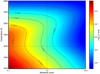 |
Fig. 6 Predicted pressure at which the atmosphere becomes optically thick to continuum radiation along the transit chord due to absorption by H−, averaged over the HARPS waveband, as a function of atmospheric temperature and metallicity. The dashed lines indicate the metallicity and temperature chosen in this study, for which the continuum is predicted to become optically thick at a pressure of 3.5 mbar. For solar metallicity, the continuum is formed between 3 and 4 mbar for temperatures between 3500 and 5500 K. For most of this parameter space, the continuum is formed between pressures of 2 and 6 mbar. This indicates that the peak pressures obtained in Table 2 are robust against errors in the assumed temperatureand metallicity to within a factor of order unity. |
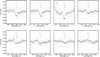 |
Fig. 7 Transmission spectrum of KELT-9 b at the location of eight strong lines of Fe II that were observed by Cauley et al. (2019). The grey points show the transmission spectrum at the native sampling of the HARPS-N instrument, while the black points are binned by 20 points. The transmission spectrum is obtained following the procedure of Wyttenbach et al. (2015), and combining all in-transit exposures of the two nights. The Doppler-shadow is removed by fitting the model described in Sect. 2 at the expected locations of the individual lines. The presence of these lines appears to be confirmed by our HARPS-N observations, but non-Gaussian systematic noise occurs at the ~ 10−3 level. This hinders the identification of all but the strongest Fe II lines. |
4.2 Individual lines of Fe II, Mg I and Na I
Strong absorption lines of Mg I and Fe II have already been observed directly in the transmission spectrum of KELT-9 b by Cauley et al. (2019) using the PEPSI spectrograph on the Large Binocular Telescope (LBT). We therefore used these HARPS-N observations to obtain the transmission spectrum of KELT-9 b using the same methods as described by Wyttenbach et al. (2015), but using a low-order polynomial to normalize the continuum (similar to Allart et al. 2017), and correcting for the Doppler-shadow in the same way as was done for the cross-correlation functions (see Sect. 2).
Figures 7 and 8 show the transmission-spectrum obtained in this way, at the location of eight strong Fe II lines also observed by Cauley et al. (2019), the Mg I triplet and the Na I-D doublet6. The strongest lines of Fe II are detected individually in the transmission spectrum, but systematic variations are present on the 10−3 level7. Excess absorption also appears around the Na I doublet, but the detection of these lines in the transmission spectrum is not robust. This highlights the advantage of using cross-correlation, in which many lines (if available) are co-added to diminish the photon noise and other noise sources that are not correlated with the target spectrum. In the optical, Na I has tradionally only been targeted through its strong resonant doublet, but at high temperatures additional transitions are also common, producing the multitude of lines that were combined in the present analysis, yielding a detection that is significantly stronger than would have been possible using only the doublet.
In addition, neutral aluminium (Al I) and ionized calcium (Ca II) have strong doublets near 390 nm (see Fig. C.1). However these were not detected because the noise at the blue edge of the HARPS-N waveband is naturally high, aggravated by the malfunction of the ADC that caused a strong loss of flux at short wavelengths in the second night of observations. Besides these two doublets, the spectra of most other species appear to be more rich at blue optical and UV wavelengths (see Fig. C.1) and we propose that future spectroscopic observations at blue/NUV wavelengths (notably with HST/STIS) have a strong potential to reveal additional absorbers in the transmission spectrum of the atmosphere of KELT-9 b.
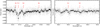 |
Fig. 8 Similar to Fig. 7, this figure shows the transmission spectrum of KELT-9 b at the location of the Mg I triplet that was observed by Cauley et al. (2019), and the Na I-D doublet, which was not covered by the observations by Cauley et al. (2019). The systematic noise at the ~ 10−3 level hampers the detection of these individual lines. |
4.3 The systemic velocity and high-altitude winds
The HARPS-N spectrograph is routinely used to monitor the radial velocity of stars with a long-term precision at the m s−1 level (Cosentino et al. 2012). For this purpose the pipeline automatically cross-correlates the spectrum of the target star with a standard binary mask, in this case a mask tailored to the spectrum of an A0 main sequence star (Nielsen et al., in prep.). Using the cross-correlation functions provided by the pipeline, we measure the radial velocity of the star in the exposures obtained before and after the transit8. For the twonights, this yields measurements of the systemic radial velocity of − 17.63 ± 0.14 and − 17.88 ± 0.16 km s−1 respectively.
Gaudi et al. (2017) report a systemic velocity of − 20.565 ± 0.1 km s−1, which is significantly discrepant from our measurements. The reason for such a discrepancy at the km s−1 level is not immediately evident, but may well be explained by differences in the cross-correlation masks used to derive the radial velocity, as well as the radial-velocity zero-points of the spectrographs. For the purpose of this study we adopted a systemic velocity of − 17.74 ± 0.11 km s−1 as the average of our two measurements.
The strong signatures of Na I, Mg I, Ti II, Cr II, Fe I and Fe II in this survey appear to have symmetrical line profiles at velocities that are consistent with the measured systemic velocity to within 3σ. Especially the Fe II line, although spanning a large range of altitudes, is consistent with the systemic velocity as it deviates from the planet rest frame velocity by 0.18 ± 0.27 km s−1. Similarly, the Fe I line is shifted by 0.84 ± 0.37 km s−1. Our detections therefore do not indicate the presence of a strong net day-to-night-side wind (the second circulation regime of Showman et al. 2013), nor a tail-like flow of the envelope material over the range of pressures probed by these lines – i.e. from the millibar to the microbar level.
4.4 The stellar mass
The detection of the absorption lines in the transmission spectrum of the planet yields a measurement of the radial velocity of the planet as a function of time during transit. Assuming a circular orbit and the known orbital period, this yields the projected orbital velocity of the planet. This was first used by Brogi et al. (2012) to measure the true orbital velocity of the non-transiting hot Jupiter τ Boo b, which was first known only up until a factor sini because the inclination of the orbit was unknown. Assuming a circular orbit, we fit the radial velocity v(t) of the peak of the cross-correlation function of Fe II in each exposure during the transit to obtain the orbital velocity vorb, up to the projection angle sini:
 (7)
(7)
where t − t0 and P are the time from transit centre time and the orbital period as provided by Gaudi et al. (2017). The resulting fit is shown in Fig. 9, and yields a projected orbital velocity of  km s−1.
Because KELT-9 b is a transiting planet, knowledge of the orbital inclination, the orbital period and the orbital velocity may be used to retrieve the true mass of the star. Rewriting Keplers third law for a circular orbit, the stellar mass M* is given by
 (8)
(8)
where mp is the mass of the planet. Filling in the measured orbital velocity and the inclination, orbital period and planet massreported by Gaudi et al. (2017), we obtain a revised measurement of the stellar mass of M* = 1.978 ± 0.023 M⊙. The uncertainty on this value is approximately ten times lower than reported by Gaudi et al. (2017), and takes into account the uncertainties on P, i and mp. The stellar density and planet-to-star radius ratio were obtained by Gaudi et al. (2017) as direct observables from the shape and depth of the transit lightcurve (Seager & Mallén-Ornelas 2003), who reported values of ρ* = 0.2702 ± 0.0029 g cm−3 and  . We are therefore able to revise the stellar radius to R* = 2.178 ± 0.011 R⊙ and the planet radius to Rp = 1.783 ± 0.009 RJ. Finally, with the revised stellar mass we also revise the mass of the planet, which is derived from the radial velocity semi-amplitude K of the star provided by Gaudi et al. (2017), assuming a circular orbit:
 (9)
(9)
which yields a mass of 2.44 ± 0.70 MJ9.
 |
Fig. 9 Radial velocity of the planet as a function of orbital phase. It is obtained by fitting the average Fe II line as a Gaussian in each exposure of each of the two nights. The blue line signifies our fit of Eq. (7), which yields a best-fit projected orbital velocity of 234.24 ± 0.90 km s−1. |
5 Conclusion
This paper presents a survey of the transmission spectrum of KELT-9 b for absorption signatures of 76 atomic species and their ions, as observed by the high-resolution echelle spectrograph HARPS-N. Of these 76 species, 18 neutrals and 21 ions are expected to have significant line absorption in the HARPS-N waveband. We modelled the absorption spectra of these species using the FastChem code (Stock et al. 2018) to model the expected composition of the atmosphere at 4000 K, and used these model spectra as cross-correlation templates to co-add the individual absorption lines of these species into average line-profiles. By doing so, we are able to report on new detections of Na I, Sc II, Cr II and Y II in the atmosphere of KELT-9 b, while confirming previous detections of Mg I, Ti I, Fe I and Fe II (Hoeijmakers et al. 2018a; Cauley et al. 2019). In addition, we find cross-correlation enhancements of Ca I, Cr I, Co I, and Sr II near the expected orbital velocity of the planet but these have low significance and/or non-Gaussian profiles. These tentative signatures will require further observations to verify.
The injection of the model templates into the data allows the strength of the cross-correlation functions to be compared to the models. From this we conclude that equilibrium chemistry at solar metallicity and 4000 K comes close to adequately explaining the observed line-depths of Fe I and Sc II. However, the strong absorption lines of the other species appear to be anomalous, especially those of Cr II and Fe II, which are both underpredicted by a factor of eight to ten. Our atmospheric model predicts that the atmosphere becomes opaque to continuum radiation at a pressure of 3.5 mbar. We could therefore derive the pressure level corresponding to the observed line-depths and find that these occur between the mbar and microbar levels. We tentatively ascribe the discrepancy between our isothermal, hydrostatic thermal equilibrium model and the data to the presence of a hydrodynamic outflow that lifts the absorbing species to higher altitudes. The presence of an escaping envelope surrounding KELT-9 b has already been confirmed by recent observations of the H-α line by Yan & Henning (2018).
From the cross-correlation performed by the HARPS-N pipeline, we constrain the systemic velocity of the KELT-9 system to − 17.74 ± 0.11 km s−1, significantly deviant from the value of − 20.565 ± 0.1 km s−1 reported by Gaudi et al. (2017). The observed absorption lines in the transmission spectrum of the planet atmosphere do not show a significant net blue-shift from the systemic velocity that would indicate a global day-to-night side wind or a tail-like structure of the envelope material at the pressures probed.
We measured the variation of the radial velocity of the planet during transit using the strong Fe II lines, and find a projected orbital velocity of 234.24 ± 0.90 km s−1. Treating thesystem like a spectroscopic binary and using the transit parameters reported by Gaudi et al. (2017), we revise the stellar mass and radius to M* = 1.978 ± 0.023 M⊙ and R* = 2.178 ± 0.011 R⊙, and the planet mass and radius to mp = 2.44 ± 0.70 MJ and Rp = 1.783 ± 0.009 RJ.
Acknowledgements
This project has received funding from the European Research Council (ERC) under the European Union’s Horizon 2020 research and innovation programme (projects Four Aces and EXOKLEIN with grant agreement numbers 724427 and 771620, respectively). This work has been carried out in the framework of the PlanetS National Centre of Competence in Research (NCCR) supported by the Swiss National Science Foundation (SNSF). Based on observations made with the Italian Telescopio Nazionale Galileo (TNG) operated on the island of La Palma by the Fundación Galileo Galilei of the INAF (Istituto Nazionale di Astrofisica) at the Spanish Observatorio del Roque de los Muchachos of the Instituto de Astrofisica de Canarias. This project has received funding from the European Union’s Horizon 2020 research and innovation programme under grant agreement No 730890 (OPTICON). This material reflects only the authors views and the Commission is not liable for any use that may be made of the information contained therein. A.W acknowledges the support of the SNSF with grant number P2GEP2_178191.
Appendix A The weighted cross-correlation
The cross-correlation c(v, t) provides an independent measurement of the average line profile for each exposure in the time-series of the observations. Hence, c(v, t) is a function of both the time of observation (or equivalently the orbital phase of the planet) and the radial velocity to which the template is shifted. This yields the two-dimensional cross-correlation maps that are regularly presented in studies that use the cross-correlation technique, for example Figs. 5, 8 and 12 in Brogi et al. (2018), Birkby et al. (2017) and Hoeijmakers et al. (2018b) respectively. c(v, t) is computedindependently for each of the wavelength bins. In our study these are 20 nm-wide sections of the stitched 1D spectra as produced by the HARPS-N pipeline, but they could also be the individual spectral orders of the echelle spectrograph. To combine these, we first take the weighted mean of c(v) over the Nb = 15 bins to produce the two-dimensional cross-correlation function over the entire spectral range, followed by a second weighted mean over the Ne = 19 exposures in-transit, yielding a one-dimensional cross-correlation C(v) function that corresponds to the mean line profile over the entire dataset:
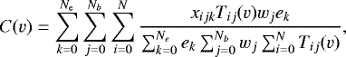 (A.1)
(A.1)
where ek is the weight assigned to the value of c(v) in exposure k, wj is the weight assigned to c(v) of each of the 15 bins, xijk is spectral data point i in bin j and exposure k, and Tij (v) is the template corresponding to each of these xijk shifted to radial velocity v.
The weights wj and ek are based on the signal-to-noise of the signal retrieved when injecting the template T into the data, broadened by the expected rotational velocity of the planet assuming tidal locking (see Sect. 3.3). The weights are thus effectively optimized to retrieve a transmission spectrum of the planet that corresponds to T, and this is done for each species independently. This assures that the spectral pixels are all co-added based on not only the expected position and strengths of the absorption lines (as follows from the forward-model of the atmosphere), but also implicitly accounting for the wavelength-dependence of noise over the spectral range. Regions with high flux and deep planetary absorption lines are thus naturally favoured over regions where the noise is higher (such as at the edges of spectral orders, at blue wavelengths and in deep stellar absorption lines), or where the planet has fewer or shallower lines.
The cross-correlation of the injected template is denoted as CI, and its absolute signal is obtained by subtracting CI − C. The peak S/N of this cross-correlation signal occurs at the radial velocity of the planet at which the template T was injected(corresponding with the true expected radial velocity of the planet in-transit), and is denoted as sjk, for each bin j and exposure k. ek is now obtained by taking the mean of s2 over j, and wj is obtained by taking the mean of s2 over k.
Appendix B Notes onnomenclature
As already noted by Pino et al. (2018b), the functional form of what is referred to as “cross-correlation” varies between fields, and the distinction is not always made clear in the exoplanet literature. Snellen et al. (2010), Brogi et al. (2012), Hoeijmakers et al. (2015) a.o. use the Pearson correlation coefficient, which is similar to Eq. (1), but normalizes xi and Ti by subtracting their mean, and carries an additional normalization over xi in the denominator. As such, this cross-correlation coefficient is unitless and bounded between −1 and 1. Its magnitde can therefore not be related directly to the amplitude of the target spectral lines, because this information has been normalized out. Relating the amplitude of the Pearson cross-correlation to a physical line-stregth therefore relies on injection (as in e.g. Hoeijmakers et al. 2015) or subtraction (as in e.g. Brogi et al. 2017) of the model template to compare the real and injected cross-correlation amplitudes.
Allart et al. (2017) and Hoeijmakers et al. (2018a) as well as the present work refer to Eq. (1) as the cross-correlation, although it is functionally identical to a weighted mean of spectral pixels, and more closely related to the cross-covariance. This function preserves the physical unit of the data (in the present case: transit depth), allowing a direct interpretation of the amplitude of the cross-correlation signal as the average line-depth (Pino et al. 2018b). The cross-covariance can also be incorporated into an expression of the likelihood function L, allowing it to be used to derive posterior distributions (Brogi et al. 2018).
Appendix C The full survey
Besides the detected species shown in Fig. 5, in Fig. C.1 we present the modelled absorption spectra of all species between atomic number three and 78 for which line-list data was available. We chose not to include elements with atomic number above 78 because the modelled spectra were mostly devoid of lines and line-list data was sparse. Figure C.2 shows the cross-correlation signature of each of the species in the same way as Fig. 5. Table C.1 shows the scaling factors by which the model of the Doppler shadow was multiplied before subtraction. Finally, Table C.2 shows the coefficients of our fits to the mass action constants used to compute the equilibrium chemistry model of the atmosphere using FastChem.
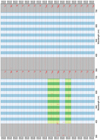 |
Fig. C.1 Modelled spectra of all neutral and singly ionized species in our survey, with the atomic number increasing downwards. The spectra are computed at solar metallicity and a temperature of 4000 K, with a continuum set by H−. The y-axis denotes transit depth, with unity equal to the out-of-transit flux of the star. The shaded grey areas demarcate the edges of the HARPS-N waveband. The alternating shaded colours indicate the 20 nm wide bands for which the cross-correlation analysis is performed independently. Green and lime highlighted species are species with significant expected line opacity and that were selected for cross-correlation. Species for which no spectrum is plotted were lacking in line-list data. |
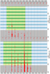 |
Fig. C.1 continued. |
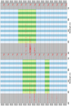 |
Fig. C.1 continued. |
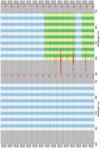 |
Fig. C.1 continued. |
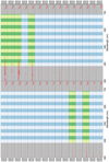 |
Fig. C.1 continued. |
 |
Fig. C.2 Cross-correlation functions of all surveyed species highlighted in Fig. C.1. The colours indicate detections (green) and non-detections (red), as well as tentative signatures that occur at the expected radial and orbital velocities of the planet, but at low confidence and/or with an irregular structure (brown). |
 |
Fig. C.2 continued. |
 |
Fig. C.2 continued. |
Scaling factors by which the model of the Doppler shadow was multiplied before subtracting it from the cross-correlation functions of each of the individual species, averaged over the two nights.
Coefficients for the fit of the temperature-dependent mass action constants of ions (including anions).
References
- Allart, R., Lovis, C., Pino, L., et al. 2017, A&A, 606, A144 [NASA ADS] [CrossRef] [EDP Sciences] [Google Scholar]
- Allart, R., Bourrier, V., Lovis, C., et al. 2018, Science, 362, 1384 [NASA ADS] [CrossRef] [Google Scholar]
- Arcangeli, J., Désert, J.-M., Line, M. R., et al. 2018, ApJ, 855, L30 [NASA ADS] [CrossRef] [Google Scholar]
- Asplund, M., Grevesse, N., Sauval, A. J., & Scott, P. 2009, ARA&A, 47, 481 [NASA ADS] [CrossRef] [Google Scholar]
- Astudillo-Defru, N., & Rojo, P. 2013, A&A, 557, A56 [NASA ADS] [CrossRef] [EDP Sciences] [Google Scholar]
- Baraffe, I., Chabrier, G., & Barman, T. 2010, Rep. Prog. Phys., 73, 016901 [NASA ADS] [CrossRef] [Google Scholar]
- Baranne, A., Queloz, D., Mayor, M., et al. 1996, A&AS, 119, 373 [NASA ADS] [CrossRef] [EDP Sciences] [Google Scholar]
- Ben-Jaffel, L., & Sona Hosseini, S. 2010, ApJ, 709, 1284 [NASA ADS] [CrossRef] [Google Scholar]
- Benneke, B., & Seager, S. 2012, ApJ, 753, 100 [NASA ADS] [CrossRef] [Google Scholar]
- Birkby, J. L., de Kok, R. J., Brogi, M., Schwarz, H., & Snellen, I. A. G. 2017, AJ, 153, 138 [NASA ADS] [CrossRef] [Google Scholar]
- Bourrier, V., Lecavelier des Etangs, A., & Vidal-Madjar, A. 2015, A&A, 573, A11 [NASA ADS] [CrossRef] [EDP Sciences] [Google Scholar]
- Brewer, J. M., Fischer, D. A., & Madhusudhan, N. 2017, AJ, 153, 83 [NASA ADS] [CrossRef] [Google Scholar]
- Brogi, M., Snellen, I. A. G., de Kok, R. J., et al. 2012, Nature, 486, 502 [NASA ADS] [CrossRef] [PubMed] [Google Scholar]
- Brogi, M., de Kok, R. J., Albrecht, S., et al. 2016, ApJ, 817, 106 [NASA ADS] [CrossRef] [Google Scholar]
- Brogi, M., Line, M., Bean, J., Désert, J.-M., & Schwarz, H. 2017, ApJ, 839, L2 [NASA ADS] [CrossRef] [Google Scholar]
- Brogi, M., Giacobbe, P., Guilluy, G., et al. 2018, A&A, 615, A16 [NASA ADS] [CrossRef] [EDP Sciences] [Google Scholar]
- Cauley, P. W., Shkolnik, E. L., Ilyin, I., et al. 2019, AJ, 157, 69 [NASA ADS] [CrossRef] [Google Scholar]
- Chase, M., & Unidos, T. E. 1998, NIST-JANAF Thermochemical Tables, Journal of physical and chemical reference data: Monograph (Washington: American Chemical Society) [Google Scholar]
- Collier Cameron, A., Guenther, E., Smalley, B., et al. 2010, MNRAS, 407, 507 [NASA ADS] [CrossRef] [Google Scholar]
- Cosentino, R., Lovis, C., Pepe, F., et al. 2012, Proc. SPIE, 8446, 84461V [Google Scholar]
- de Wit, J., & Seager, S. 2013, Science, 342, 1473 [NASA ADS] [CrossRef] [Google Scholar]
- Ehrenreich, D., Bourrier, V., Bonfils, X., et al. 2012, A&A, 547, A18 [NASA ADS] [CrossRef] [EDP Sciences] [Google Scholar]
- Ehrenreich, D., Bourrier, V., Wheatley, P. J., et al. 2015, Nature, 522, 459 [Google Scholar]
- Fisher, C., & Heng, K. 2018, MNRAS, 481, 4698 [Google Scholar]
- Fortney, J. J., Shabram, M., Showman, A. P., et al. 2010, ApJ, 709, 1396 [NASA ADS] [CrossRef] [Google Scholar]
- Fossati, L., Bagnulo, S., Elmasli, A., et al. 2010, ApJ, 720, 872 [NASA ADS] [CrossRef] [Google Scholar]
- Fossati, L., Koskinen, T., Lothringer, J. D., et al. 2018, ApJ, 868, L30 [NASA ADS] [CrossRef] [Google Scholar]
- Gaidos, E., Kitzmann, D., & Heng, K. 2017, MNRAS, 468, 3418 [NASA ADS] [CrossRef] [Google Scholar]
- Gaudi, B. S., Stassun, K. G., Collins, K. A., et al. 2017, Nature, 546, 514 [NASA ADS] [Google Scholar]
- Genova, F., Egret, D., Bienaymé, O., et al. 2000, A&AS, 143, 1 [NASA ADS] [CrossRef] [EDP Sciences] [Google Scholar]
- Griffith, C. A. 2014, Phil. Trans. R. Soc. London, Ser. A, 372, 20130086 [Google Scholar]
- Grimm, S. L., & Heng, K. 2015, ApJ, 808, 182 [NASA ADS] [CrossRef] [Google Scholar]
- Gurvich, L. V., Veits, I. V., Medvedev, V. A., et al. 1982, Thermodynamic Properties of Individual Substances, 4, ed. V. P. Glushko (Nauka: Moscow) [Google Scholar]
- Haswell, C. A., Fossati, L., Ayres, T., et al. 2012, ApJ, 760, 79 [NASA ADS] [CrossRef] [Google Scholar]
- Heng, K., & Kitzmann, D. 2017, MNRAS, 470, 2972 [NASA ADS] [CrossRef] [Google Scholar]
- Heng, K., Wyttenbach, A., Lavie, B., et al. 2015, ApJ, 803, L9 [Google Scholar]
- Hoeijmakers, H. J., de Kok, R. J., Snellen, I. A. G., et al. 2015, A&A, 575, A20 [NASA ADS] [CrossRef] [EDP Sciences] [Google Scholar]
- Hoeijmakers, H. J., Ehrenreich, D., Heng, K., et al. 2018a, Nature, 560, 453 [NASA ADS] [CrossRef] [Google Scholar]
- Hoeijmakers, H. J., Snellen, I. A. G., & van Terwisga, S. E. 2018b, A&A, 610, A47 [NASA ADS] [CrossRef] [EDP Sciences] [Google Scholar]
- Huang, C., Arras, P., Christie, D., & Li, Z.-Y. 2017, ApJ, 851, 150 [NASA ADS] [CrossRef] [Google Scholar]
- Huitson, C. M., Sing, D. K., Vidal-Madjar, A., et al. 2012, MNRAS, 422, 2477 [NASA ADS] [CrossRef] [Google Scholar]
- Husser, T.-O., Wende-von Berg, S., Dreizler, S., et al. 2013, A&A, 553, A6 [NASA ADS] [CrossRef] [EDP Sciences] [Google Scholar]
- John, T. L. 1988, A&A, 193, 189 [NASA ADS] [Google Scholar]
- Kempton, E. M.-R., Perna, R., & Heng, K. 2014, ApJ, 795, 24 [NASA ADS] [CrossRef] [Google Scholar]
- Kitzmann, D., Heng, K., Rimmer, P. B., et al. 2018, ApJ, 863, 183 [NASA ADS] [CrossRef] [Google Scholar]
- Koen, C., Balona, L. A., Khadaroo, K., et al. 2003, MNRAS, 344, 1250 [NASA ADS] [CrossRef] [Google Scholar]
- Kramida, A., Ralchenko, Y., Nave, G., & Reader, J. 2018a, APS Meeting Abstracts, M01.004 [Google Scholar]
- Kramida, A., Ralchenko, Y., Reader, J., & NIST ASD Team 2018b, NIST Atomic Spectra Database (ver. 5.6.1), https://physics.nist.gov/asd (2015, April 16), National Institute of Standards and Technology, Gaithersburg, MD. [Google Scholar]
- Kreidberg, L., Line, M. R., Bean, J. L., et al. 2015, ApJ, 814, 66 [NASA ADS] [CrossRef] [Google Scholar]
- Kulow, J. R., France, K., Linsky, J., & Loyd, R. O. P. 2014, ApJ, 786, 132 [NASA ADS] [CrossRef] [Google Scholar]
- Kurucz, R. L. 2018, ASP Conf. Ser., 515, 47 [NASA ADS] [Google Scholar]
- Kurucz, R. L., & Bell, B. 1995, Atomic Line List (Cambridge, MA: Smithsonian Astrophysical Observatory) [Google Scholar]
- Lecavelier Des Etangs, A., Pont, F., Vidal-Madjar, A., & Sing, D. 2008, A&A, 481, L83 [NASA ADS] [CrossRef] [Google Scholar]
- Lide, D. R. 2004, CRC Handbook of Chemistry and Physics, 85th edn. (Boca Raton: CRC Press) [Google Scholar]
- Linsky, J. L., Yang, H., France, K., et al. 2010, ApJ, 717, 1291 [NASA ADS] [CrossRef] [Google Scholar]
- Lothringer, J. D., Barman, T., & Koskinen, T. 2018, ApJ, 866, 27 [NASA ADS] [CrossRef] [Google Scholar]
- Louden, T., & Wheatley, P. J. 2015, ApJ, 814, L24 [NASA ADS] [CrossRef] [Google Scholar]
- Madhusudhan, N., Amin, M. A., & Kennedy, G. M. 2014, ApJ, 794, L12 [Google Scholar]
- Mendonça, J. M., Tsai, S.-m., Malik, M., Grimm, S. L., & Heng, K. 2018, ApJ, 869, 107 [NASA ADS] [CrossRef] [Google Scholar]
- Miller-Ricci Kempton, E., & Rauscher, E. 2012, ApJ, 751, 117 [NASA ADS] [CrossRef] [Google Scholar]
- Mordasini, C., van Boekel, R., Mollière, P., Henning, T., & Benneke, B. 2016, ApJ, 832, 41 [NASA ADS] [CrossRef] [Google Scholar]
- Nikolov, N., Sing, D. K., Fortney, J. J., et al. 2018, Nature, 557, 526 [NASA ADS] [CrossRef] [Google Scholar]
- Nortmann, L., Pallé, E., Salz, M., et al. 2018, Science, 362, 1388 [NASA ADS] [CrossRef] [EDP Sciences] [Google Scholar]
- Oklopčić, A., & Hirata, C. M. 2018, ApJ, 855, L11 [NASA ADS] [CrossRef] [Google Scholar]
- Parmentier, V., Line, M. R., Bean, J. L., et al. 2018, A&A, 617, A110 [NASA ADS] [CrossRef] [EDP Sciences] [Google Scholar]
- Pepe, F., Mayor, M., Galland, F., et al. 2002, A&A, 388, 632 [NASA ADS] [CrossRef] [EDP Sciences] [Google Scholar]
- Pino, L., Ehrenreich, D., Wyttenbach, A., et al. 2018a, A&A, 612, A53 [NASA ADS] [CrossRef] [EDP Sciences] [Google Scholar]
- Pino, L., Ehrenreich, D., Allart, R., et al. 2018b, A&A, 619, A3 [NASA ADS] [CrossRef] [EDP Sciences] [Google Scholar]
- Redfield, S., Endl, M., Cochran, W. D., & Koesterke, L. 2008, ApJ, 673, L87 [NASA ADS] [CrossRef] [MathSciNet] [Google Scholar]
- Richard, C., Gordon, I. E., Rothman, L. S., et al. 2012, J. Quant. Spectr. Rad. Transf., 113, 1276 [NASA ADS] [CrossRef] [Google Scholar]
- Saha, M. 1920, London Edinburgh Dublin Philos. Mag. J. Sci., 40, 472 [CrossRef] [Google Scholar]
- Salz, M., Czesla, S., Schneider, P. C., et al. 2018, A&A, 620, A97 [NASA ADS] [CrossRef] [EDP Sciences] [Google Scholar]
- Schlawin, E., Agol, E., Walkowicz, L. M., Covey, K., & Lloyd, J. P. 2010, ApJ, 722, L75 [NASA ADS] [CrossRef] [Google Scholar]
- Seager, S., & Mallén-Ornelas, G. 2003, ApJ, 585, 1038 [NASA ADS] [CrossRef] [Google Scholar]
- Seidel, J. V., Ehrenreich, D., Wyttenbach, A., et al. 2019, A&A, 623, A166 [NASA ADS] [CrossRef] [EDP Sciences] [Google Scholar]
- Showman, A. P., Fortney, J. J., Lian, Y., et al. 2009, ApJ, 699, 564 [NASA ADS] [CrossRef] [Google Scholar]
- Showman, A. P., Fortney, J. J., Lewis, N. K., & Shabram, M. 2013, ApJ, 762, 24 [NASA ADS] [CrossRef] [Google Scholar]
- Sing, D. K., Vidal-Madjar, A., Lecavelier des Etangs, A., et al. 2008, ApJ, 686, 667 [NASA ADS] [CrossRef] [Google Scholar]
- Smette, A., Sana, H., Noll, S., et al. 2015, A&A, 576, A77 [NASA ADS] [CrossRef] [EDP Sciences] [Google Scholar]
- Snellen, I. A. G., de Kok, R. J., de Mooij, E. J. W., & Albrecht, S. 2010, Nature, 465, 1049 [NASA ADS] [CrossRef] [PubMed] [Google Scholar]
- Spake, J. J., Sing, D. K., Evans, T. M., et al. 2018, Nature, 557, 68 [NASA ADS] [CrossRef] [EDP Sciences] [Google Scholar]
- Spiegel, D. S., Silverio, K., & Burrows, A. 2009, ApJ, 699, 1487 [NASA ADS] [CrossRef] [Google Scholar]
- Stock, J. W., Kitzmann, D., Patzer, A. B. C., & Sedlmayr, E. 2018, MNRAS, 479, 865 [NASA ADS] [Google Scholar]
- Tsai, S.-M., Lyons, J. R., Grosheintz, L., et al. 2017, ApJS, 228, 20 [NASA ADS] [CrossRef] [Google Scholar]
- Vidal-Madjar, A., Lecavelier des Etangs, A., Désert, J.-M., et al. 2003, Nature, 422, 143 [NASA ADS] [CrossRef] [PubMed] [Google Scholar]
- Vidal-Madjar, A., Désert, J.-M., Lecavelier des Etangs, A., et al. 2004, ApJ, 604, L69 [NASA ADS] [CrossRef] [Google Scholar]
- Vidal-Madjar, A., Sing, D. K., Lecavelier Des Etangs, A., et al. 2011, A&A, 527, A110 [Google Scholar]
- Wyttenbach, A., Ehrenreich, D., Lovis, C., Udry, S., & Pepe, F. 2015, A&A, 577, A62 [NASA ADS] [CrossRef] [EDP Sciences] [Google Scholar]
- Wyttenbach, A., Lovis, C., Ehrenreich, D., et al. 2017, A&A, 602, A36 [NASA ADS] [CrossRef] [EDP Sciences] [Google Scholar]
- Yan, F., & Henning, T. 2018, Nat. Astron., 2, 714 [NASA ADS] [CrossRef] [Google Scholar]
- Yan, F., Pallé, E., Fosbury, R. A. E., Petr-Gotzens, M. G., & Henning, T. 2017, A&A, 603, A73 [NASA ADS] [CrossRef] [EDP Sciences] [Google Scholar]
We chose to limit the survey to elements lighter than platinum because spectral data becomes sparse and elemental abundances diminish for elements with higher atomic numbers. Helium is not expected to feature strong lines in the optical, and the strong hydrogen lines will be treated in a separate study.
The HARPS range is divided into 15 bins of 20 nm each, with the reddest few nm being ignored due to the presence of the strong oxygen band near 687 nm.
A box-smooth or top-hat filter in velocity space is equivalent to convolution with a normalized kernel that has a non-zero value for velocities smaller than some limiting velocity, i.e. |v| < vlimit, and is equal to zero elsewhere.
Ideally, the spectra produced by the forward-models would be fit directly to the high-resolution spectra. However, an efficient sampling of parameter space is currently not computationally tractable due to the size of the high-resolution spectra.
In this high-temperature regime the term photo-chemistry loosely equates to photo-ionization because molecules are predominantly dissociated.
Single lines and simple line systems like doublets and triplets are more amenable for a targeted analysis that is applied directly to the transmission-spectrum (like e.g. Wyttenbach et al. 2015) rather than cross-correlation, because cross-correlation relies on the co-addition of many individual lines.
The origin of these systematic variations is presently unknown and may be related to the malfunction of the ADC. The magnitude of the variations exceeds the magnitude of the Doppler shadow, meaning that inaccuracies in the removal of the Doppler shadow effect cannot (fully) account for this systematic noise.
The in-transit exposures are left out as to prevent the presence of the planet to bias the velocity measurement.
The planet mass mp recurs in Eq. (8) for the mass of the star, but the adjustment in the planet mass compared to Gaudi et al. (2017) is so small that it has no effect on the initial outcome for M*. Had the planet been significantly heavier, M* and mp would have been derived iteratively.
All Tables
Scaling factors by which the model of the Doppler shadow was multiplied before subtracting it from the cross-correlation functions of each of the individual species, averaged over the two nights.
Coefficients for the fit of the temperature-dependent mass action constants of ions (including anions).
All Figures
|
Fig. 1 Mean out-of-transit spectrum of the KELT-9 system as observed by HARPS-N, produced by stitching together the individual spectral orders after correction of the blaze function. The blue and black lines show the spectrum before and after telluric correction. The smaller panel shows the telluric water band that is highlighted in grey in detail, demonstrating the effect of the telluric correction. The outlying points are residuals of deep telluric absorption and a small number of emission lines that have remained uncorrected. |
| In the text | |
|
Fig. 2 Removal of the Doppler shadow for the first night of data. Top panel: two-dimensional cross-correlation function as obtained when using a PHOENIX 10 000 K stellar atmosphere model template. The dark feature near − 40 km s−1 is the Doppler shadow caused by the planet obscuring part of the disc-integrated stellar line, that is broadened by v sin i = 111.4 km s−1 (Gaudi et al. 2017). The bright linear slanted feature is the signature of the atmosphere of the planet. It appears in this cross-correlation because the star and the planet have ionized lines in common (Hoeijmakers et al. 2018a). It is ignored when constructing and fitting the model of the Doppler shadow. Besides these, there are significant cross-correlation residuals due to stellar line-shape variations that we tentatively attribute to pulsations of KELT-9 that are not characterized in the literature as of yet, but seem to resemble those that have been observed in hot δ Scuti stars such as β Pictoris (Koen et al. 2003) and Wasp-33 (Collier Cameron et al. 2010). Middle panel: full model as fit to this cross-correlation function, where the dashed line indicates the polynomial fit to the centroid velocities of the main shadow feature in each exposure. Bottom panel: residuals after removal. |
| In the text | |
|
Fig. 3 Abundance profiles modelled with FastChem for a selection of neutral atoms (solid lines) and ions (dashed lines), as well as molecules, H− and electrons. The model assumes an isothermal structure at 4000 K and solar metallicity. Over most of the modelled pressure region, molecules tend to be dissociated and metals tend to be singly ionized. The decrease of ion abundances towards higher altitudes (pressures below ~ 10−12 bars) indicates the emergence of doubly ionized species at low pressures. The effects of photo-ionization are not included, as these are predicted to be small in the denser parts of the atmosphere (Kitzmann et al. 2018). |
| In the text | |
|
Fig. 4 Sample of model spectra of Fe I, Fe II, Ti I and Ti II in green, brown, red and blue respectively, over a 13 nm slice of the HARPS-N spectral range. These spectra are calculated assuming an isothermal atmosphere at 4000 K between pressures of 10 to 10−15 bars and abundances correponding to the solar metallicity value (Sect. 3.3). A full overview of all the calculated model spectra is provided in Fig. C.1. Together, these figures serve to show the rich absorption spectra caused by the presence of these atoms in the atmosphere of KELT-9 b. |
| In the text | |
|
Fig. 5 Cross-correlation signatures of Na I, Mg I, Sc II, Ti II, Cr II, Fe I, Fe II and Y II averaged over both nights of observation. Each row of panels is associated with one species. Left panel in each row: two-dimensional cross-correlation function c(v, t), in which thesignature of the transiting planet atmosphere has a slanted shape, as is most evident in the case of Fe I, Fe II and Ti II that were previously reported in Hoeijmakers et al. (2018a). Middle panel in each row: co-addition obtained by summing the in-transit exposures to the rest-frame velocity of the planet, assuming a range of orbital velocities, Kp. The white dashed lines indicate the expected systemic velocity, vsys (see Sect. 4.3) and orbital velocity (see Sect. 4.4). Right-most panel: one-dimensional cross-correlation function co-added in the rest-frame corresponding to the expected orbital velocity of the planet. The green line denotes the average cross-correlation over both observing nights. The dashed black line is a Gaussian fit to the profiles, with the resulting best-fit parameters provided in Table 2. The dotted red line is the signature of the injected model template. Apart from Fe I, all observed absorption lines appear to be significantly deeper than predicted for a 4000 K solar metallicity model in chemical equilibrium. The cross-correlation enhancement ~ 80 km s−1 redward of the Mg I line is caused by a strong Fe II line, which is also indicated in Fig. 7. |
| In the text | |
|
Fig. 6 Predicted pressure at which the atmosphere becomes optically thick to continuum radiation along the transit chord due to absorption by H−, averaged over the HARPS waveband, as a function of atmospheric temperature and metallicity. The dashed lines indicate the metallicity and temperature chosen in this study, for which the continuum is predicted to become optically thick at a pressure of 3.5 mbar. For solar metallicity, the continuum is formed between 3 and 4 mbar for temperatures between 3500 and 5500 K. For most of this parameter space, the continuum is formed between pressures of 2 and 6 mbar. This indicates that the peak pressures obtained in Table 2 are robust against errors in the assumed temperatureand metallicity to within a factor of order unity. |
| In the text | |
|
Fig. 7 Transmission spectrum of KELT-9 b at the location of eight strong lines of Fe II that were observed by Cauley et al. (2019). The grey points show the transmission spectrum at the native sampling of the HARPS-N instrument, while the black points are binned by 20 points. The transmission spectrum is obtained following the procedure of Wyttenbach et al. (2015), and combining all in-transit exposures of the two nights. The Doppler-shadow is removed by fitting the model described in Sect. 2 at the expected locations of the individual lines. The presence of these lines appears to be confirmed by our HARPS-N observations, but non-Gaussian systematic noise occurs at the ~ 10−3 level. This hinders the identification of all but the strongest Fe II lines. |
| In the text | |
|
Fig. 8 Similar to Fig. 7, this figure shows the transmission spectrum of KELT-9 b at the location of the Mg I triplet that was observed by Cauley et al. (2019), and the Na I-D doublet, which was not covered by the observations by Cauley et al. (2019). The systematic noise at the ~ 10−3 level hampers the detection of these individual lines. |
| In the text | |
|
Fig. 9 Radial velocity of the planet as a function of orbital phase. It is obtained by fitting the average Fe II line as a Gaussian in each exposure of each of the two nights. The blue line signifies our fit of Eq. (7), which yields a best-fit projected orbital velocity of 234.24 ± 0.90 km s−1. |
| In the text | |
|
Fig. C.1 Modelled spectra of all neutral and singly ionized species in our survey, with the atomic number increasing downwards. The spectra are computed at solar metallicity and a temperature of 4000 K, with a continuum set by H−. The y-axis denotes transit depth, with unity equal to the out-of-transit flux of the star. The shaded grey areas demarcate the edges of the HARPS-N waveband. The alternating shaded colours indicate the 20 nm wide bands for which the cross-correlation analysis is performed independently. Green and lime highlighted species are species with significant expected line opacity and that were selected for cross-correlation. Species for which no spectrum is plotted were lacking in line-list data. |
| In the text | |
|
Fig. C.1 continued. |
| In the text | |
|
Fig. C.1 continued. |
| In the text | |
|
Fig. C.1 continued. |
| In the text | |
|
Fig. C.1 continued. |
| In the text | |
|
Fig. C.2 Cross-correlation functions of all surveyed species highlighted in Fig. C.1. The colours indicate detections (green) and non-detections (red), as well as tentative signatures that occur at the expected radial and orbital velocities of the planet, but at low confidence and/or with an irregular structure (brown). |
| In the text | |
|
Fig. C.2 continued. |
| In the text | |
|
Fig. C.2 continued. |
| In the text | |
Current usage metrics show cumulative count of Article Views (full-text article views including HTML views, PDF and ePub downloads, according to the available data) and Abstracts Views on Vision4Press platform.
Data correspond to usage on the plateform after 2015. The current usage metrics is available 48-96 hours after online publication and is updated daily on week days.
Initial download of the metrics may take a while.