| Issue |
A&A
Volume 627, July 2019
|
|
|---|---|---|
| Article Number | A166 | |
| Number of page(s) | 9 | |
| Section | Interstellar and circumstellar matter | |
| DOI | https://doi.org/10.1051/0004-6361/201834430 | |
| Published online | 18 July 2019 | |
Nonthermal emission from the reverse shock of the youngest Galactic supernova remnant G1.9+0.3
1
DESY,
15738 Zeuthen, Germany
e-mail: robert.brose@mail.de
2
Institute of Physics and Astronomy, University of Potsdam,
14476 Potsdam, Germany
3
Centre for Space Research, North-West University,
2520 Potcheftroom, South Africa
4
Astronomical Observatory of Ivan Franko National University of L’viv,
vul. Kyryla i Methodia, 8,
L’viv 79005, Ukraine
5
Western Sydney University,
Locked Bag 1797, Penrith NSW 2751, Australia
6
Sorbonne University,
4 place Jussieu, 75005 Paris, France
7
Université de Versailles Saint-Quentin-en-Yvelines,
45 rue des États-Unis, 78000 Versailles, France
Received:
15
October
2018
Accepted:
29
May
2019
Context. The youngest Galactic supernova remnant G1.9+0.3 is an interesting target for next-generation gamma-ray observatories. So far, the remnant is only detected in the radio and the X-ray bands, but its young age of ≈100 yr and inferred shock speed of ≈14 000 km s−1 could make it an efficient particle accelerator.
Aims. We aim to model the observed radio and X-ray spectra together with the morphology of the remnant. At the same time, we aim to estimate the gamma-ray flux from the source and evaluate the prospects of its detection with future gamma-ray experiments.
Methods. We performed spherical symmetric 1D simulations with the RATPaC code, in which we simultaneously solved the transport equation for cosmic rays, the transport equation for magnetic turbulence, and the hydro-dynamical equations for the gas flow. Separately computed distributions of the particles accelerated at the forward and the reverse shock were then used to calculate the spectra of synchrotron, inverse Compton, and pion-decay radiation from the source.
Results. The emission from G1.9+0.3 can be self-consistently explained within the test-particle limit. We find that the X-ray flux is dominated by emission from the forward shock while most of the radio emission originates near the reverse shock, which makes G1.9+0.3 the first remnant with nonthermal radiation detected from the reverse shock. The flux of very-high-energy gamma-ray emission from G1.9+0.3 is expected to be close to the sensitivity threshold of the Cherenkov Telescope Array. The limited time available to grow large-scale turbulence limits the maximum energy of particles to values below 100 TeV, hence G1.9+0.3 is not a PeVatron.
Key words: acceleration of particles / turbulence / ISM: supernova remnants / gamma rays: ISM
© ESO 2019
1 Introduction
The approximately 100-yr-old supernova remnant (SNR) G1.9+0.3 is presumably the youngest SNR in our Galaxy. It was first detected in the radio band by Green & Gull (1984) and in X-rays by Reynolds et al. (2008). The measured gas column density places the remnant close to the Galactic center at about 8.5 kpc and strong absorption in the optical band led to the nondetection of the supernova explosion. The seemingly circular shell has a radius of about 1.75 pc and an inferred expansion velocity of about 11 000 km s−1 at this distance (Green et al. 2008).
The radio shell of G1.9+0.3 shows a strong north-south (N-S) asymmetry with the brighter rim towards the north and the dimmer rim towards the south. Radio measurements showed a brightening of G1.9+0.3 with an annual flux increase of about 1.2% yr−1 (Murphy et al. 2008) that seems to be ongoing (Luken et al., in prep.). Radio observations of G1.9+0.3 now span roughly one third of the lifespan of the SNR, promising unique insight into the underlying processes.
The X-ray structure of G1.9+0.3 consists of a main shell with a radius of about 2 pc and symmetric extensions on the E and W sides that extend to about 2.2 pc (Reynolds et al. 2008). Proper-motion measurements of the X-ray features revealed a highly anisotropic expansion of the remnant with the fastest expansion in the east-west (E-W) direction at speeds up to 15 000 km s−1 (Borkowski et al. 2017). Thermal emission from intermediate-mass elements and iron reveals an asymmetric distribution with prominent Fe Kα emission from the northern, radio-bright rim (Borkowski et al. 2013). The asymmetric distribution of ejecta hints at a highly asymmetric explosion, which could explain the radio N-S asymmetry. A gradient in the density of the ambient medium would be an alternative explanation.
So far no detection of gamma-ray emission has been reported by H.E.S.S. or Fermi (H.E.S.S. Collaboration 2014) which constrains the average magnetic-field strength inside the remnant to B > 17 μG.
Aharonian et al. (2017) analyzed the acceleration efficiency of particles in G1.9+0.3 using the synchrotron emission and found that it is only 5% of the efficiency expected for Bohm-like diffusion, whereas values close to 100% were deduced for the slightly older SNRs Cas A (Zirakashvili et al. 2014) and RX J1713.4-3946 (Zirakashvili & Aharonian 2010).
Modeling of the particle acceleration in G1.9+0.3 by Pavlović (2017) showed that the spectral-energy distribution and the brightening rate of the remnant can be explained using nonlinear diffusive shock acceleration (NDSA). However, the injection fraction of nonthermal particles entering the NDSA process must be rather high, otherwise the shock modification is too weak to reproduce the observed radio spectral index. Both published models assume that there is only one population of particles accelerated at one shock, which is in tension with the observed morphology of the remnant as the X-ray emission would peak right at the shock and the radio-emission would peak slightly inward by a few percent of the shock radius, Rs. The observed separation of the two intensity peaks is on the order of 0.25 Rsh (Reynolds et al. 2008).
Efficient particle acceleration to PeV-energies might only take place during the very early stages of SNR evolution (Bell et al. 2013, and references therein). The very young age of G1.9+0.3 combined with the high expansion velocity of about 14 000 km s−1 make this Galactic SNR a prime PeVatron candidate and a primary target for observations of the Cherenkov Telescope Array (CTA; Cherenkov Telescope Array Consortium 2017).
The aim of this paper is to model the broadband emission of G1.9+0.3 and to explain the morphology and the observed radio-brightening. To do so we combine high-resolution hydrodynamical simulations based on the Pluto code (Mignone et al. 2007) with time-dependent 1D simulations of the particle acceleration at forward and reverse shock of the SNR, as well as the transport of magnetic turbulence using our RATPaC (Radiation Acceleration and Transport Parallel Code) framework. We show that the large radial separation between the intensity peaks of radio and X-ray emission indicates that a sizable fraction of the emission originates at the reverse shock, as expected for young SNRs (Telezhinsky et al. 2012a).
In Sects. 2.1, 2.2, and 2.4 we describe our treatment of particle acceleration, magnetic turbulence, and hydrodynamical flow profiles. In Sect. 3.1 we discuss a simple one-shock model and in Sect. 3.2 a two-shock model including the self-consistent amplification of turbulence at the forward shock. Our findings are then summarized in Sect. 4.
2 Modeling
2.1 Particle acceleration
We model the acceleration of cosmic rays using a kinetic approach in the test-particle approximation (Telezhinsky et al. 2012a,b, 2013), always keeping the cosmic-ray pressure below 10% (Kang & Ryu 2010) of the shock ram pressure. The time-dependent transport equation for the differential number density of cosmic rays N (Skilling 1975) is given by
 (1)
(1)
where Dr denotes the spatial diffusion coefficient, u the advective velocity, ṗ energy losses, and Q the source of thermal particles.
We solve this transport equation in spherical symmetry and in a frame co-moving with the shock. The radial coordinate is transformed according to , where x = r∕Rsh and Rsh is the shock radius. For an equidistant binning of x* this transformation guarantees a very fine resolution close to the shock, where Δr = 10−6 × Rsh. At the same time the outer grid-boundary extends to several tens of shock-radii upstream for x* ≫ 1. Thus, all accelerated particles can be kept in the simulation domain.
The injection of particles is determined by the source term,
 (2)
(2)
where η is the injection efficiency parameter, nu is the plasma number density in the upstream region, Vsh is the shock speed, Vu is the plasma velocity in the upstream region, and pinj = ξpth is the injection momentum, defined as a multiple of the mean thermal momentum of the plasma-particles with the temperature Td,  . For cosmic-ray protons we use the parametrization of Blasi et al. (2005) for the thermal-leakage injection model. Here pinj is the minimum momentum above which particles can cross the shock and participate in the acceleration process. For a strong shock with a compression ratio of 4, the injection efficiency is determined by
 (3)
(3)
We inject all particles with momentum pinj at the position of the shock. The injection parameter ξ determines the normalization of the resulting particle spectra and, in the case of a self-consistent treatment of Alfvénic turbulence, the maximum energy of the cosmic rays (CR). If ξ were the same forelectrons and for protons, the resulting electron-to-proton ratio at high energies would be determined by the mass ratio, 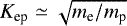 (Pohl 1993). Strictly speaking, thermal leakage cannot be the only injection mechanism for electrons. The shock thickness is commensurate with the gyro radius of the incoming protons, that is, rL = Vsh ∕ Ωp, and only particles with Larmor radii a few times that see the shock as a discontinuity and can be accelerated by DSA. For typical SNR shock speeds, electrons only get injected into the DSA process if their momentum is above a few tens of MeV c−1, that is, their momentum is larger than the thermal momentum of the protons and ξe ≫ξp. However, a fraction of the electrons might be pre-accelerated at the shock, for instance by shock-surfing acceleration or shock drift acceleration (Matsumoto et al. 2012; Matsumoto et al. 2017; Bohdan et al. 2017), enabling their participation in DSA. Thermal leakage of electrons is hence a gross simplification of complicated processes, but as the relevant parameters in our model are the number of injected particles and the electron-to-proton-ratio, a detailed account of the electron pre-acceleration is not needed, and we treat the initial pre-acceleration at the shock like DSA.
We separately solve the transport equations for the forward and reverse shock. We treat both shocks independently as there is little exchange of CRs through the contact discontinuity. The two particle distributions are then combined to calculate the total emission from the remnant.
Here, we consider two realizations of the diffusion coefficient. The first option is to assume Bohm diffusion close to the shock and in the downstream region, and to have a transition to the Galactic diffusion coefficient further upstream. In this case the diffusion coefficient is given by
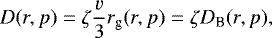 (4)
(4)
where rg is the gyro-radius of the particle, v the particles velocity, ζ a free scaling parameter, and DB the diffusion coefficient in the Bohm-limit. Here, ζ = 1 represents the lowest diffusion coefficient possible in a given magnetic field and ζ > 1 might be a more common situation. Alternatively, the amplification of Alfvénic turbulence can be explicitly treated by solving a separate wave transport equation and thus calculating the diffusion coefficient self-consistently (Brose et al. 2016).
2.2 Magnetic turbulence
There are potentially a number of wave modes that can scatter CRs inside and upstream of SNRs. While small-scale nonresonant modes can be produced very efficiently (Lucek & Bell 2000; Bell 2004), they are not able to scatter the most energetic particles in the system via resonant interactions unless efficient mode-conversion is established. This makes it unclear whether or not these modes can support the increase of the maximum energy of the CRs in the SNR.
Alfvén waves have been discussed as scattering centers for CRs in SNRs for a long time. In this paper we consider isotropic Alfvén waves as scattering centers for CRs. The transport of magnetic turbulence can be described by a continuity equation for the spectral energy density, Ew = Ew(r, k, t),
![\begin{align*} & \frac{\partial E_{\textrm{w}}{{(r,k,t)}}}{\partial t} + \mathbf{u} \cdot (\nabla E_{\textrm{w}}) + (\nabla \cdot \mathbf{u})E_{\textrm{w}} + k\frac{\partial}{\partial k}\left( \mathbf{k^2} D_{\textrm{k}} \frac{\partial}{\partial k} \frac{E_{\textrm{w}}}{k^3}\right)\nonumber\\[2pt] &\quad =2(\Gamma_{\textrm{g}}-\Gamma_{\textrm{d}})E_{\textrm{w}},\end{align*}](/articles/aa/full_html/2019/07/aa34430-18/aa34430-18-eq8.png) (5)
(5)
where Dk is the diffusion coefficient in wavenumber space representing cascading and Γg and Γd are the growth and the damping rates, respectively (Brose et al. 2016, and references therein).
We are thus able to track the growth and damping, the cascading, compression, and the propagation of the Alfvénic turbulence in the CR precursor and inside the SNR. The transport equation for the magnetic turbulence Eq. (5) is solved in parallel to the CR transport Eq. (1) for cosmic rays and the hydrodynamic equations. It is also transformedto a frame co-moving with the shock and solved in 1D under spherical symmetry, leading to a system of coupled equations which we numerically solve using implicit finite-difference methods provided by FiPy (Guyer et al. 2009).
We onlyconsider resonant interactions between waves and CRs. The resonance condition is
 (6)
(6)
where kres is the wavenumber, q the particle charge, and B0 the amplitude of the background magnetic field.
Alfvén waves can be generated by particles streaming faster than the Alfvén speed, vA. The generated waves have wavelengths similar to the gyro-radii of the particles (Wentzel 1974, and references therein). This mechanism, known as resonant amplification of Alfvén waves, is the only wave-driving process considered in this work. In the diffusion limit, the growth rate of the waves can be related to the pressure gradient of the CRs. The growth rate due to resonant amplification is given as (Skilling 1975; Bell 1978)
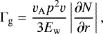 (7)
(7)
where Eq. (6) provides the link between p and k. For wave damping we consider only ion-cyclotron damping, as the young age of the remnant and the absence of a region with a low temperaturemakes neutral-charge collisions an inefficient damping process. The interaction of Alfvén is strongest at small scales,
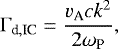 (8)
(8)
where ωP is the ion plasma frequency (Threlfall et al. 2011). This mechanism should heat the plasma, which is not included in this work, though we are aware that it might modify the spectrum near the injection momentum.
The energy transfer between turbulence of different scales is not yet fully understood and is the subject of ongoing research. If shocks are not involved, this energy transfer can be empirically described as a diffusion process in wavenumber space (Zhou & Matthaeus 1990; Schlickeiser 2002). Given our assumption of isotropic turbulence, the corresponding diffusion coefficient is
 (9)
(9)
If cascading is the dominant process, this phenomenological treatment will result in a Kolmogorov-like turbulence spectrum, Ew ∝ k−2∕3.
The term for the amplification of turbulence in Eq. (5) requires some sort of seed turbulence for which we derive a spectrum from an assumed diffusion coefficient as initial condition,
 (10)
(10)
The value of D0 is lower by a factor 100 than the ISM diffusion coefficient found in studies of Galactic CR propagation to improve the numerical stability of the code (e.g. Trotta et al. 2011).
The amplified turbulence contributes to the overall magnetic field in the remnant and can play a crucial role in the acceleration and the emission processes. The effective magnetic-field strength, Btot, is given by
![\begin{align*} &B_{\mathrm{tot}}^2 = B_0^2+\langle \delta b^2\rangle,\\[0pt]\end{align*}](/articles/aa/full_html/2019/07/aa34430-18/aa34430-18-eq14.png) (11)
where
(11)
where
 (12)
(12)
We are aware that we overestimate the guide magnetic field experienced by high-energy particles and long-wavelength waves in this way. Both effects have little impact and additionally act in a way to partially compensate each other.
It has been shown that additional magnetic turbulence can be generated downstream of the SNR shock by various MHD processes (Fraschetti 2014, and references therein). We included the possibility of such mechanisms by injecting large-scale turbulence downstream of the shock as a delta function in wave-number space.
 (13)
(13)
where κ ≈ 1% determines the fraction of the downstream thermal energy that is transferred to magnetic-field energy, and ki = 3.1 × 10⁻¹⁷ cm−1 and Δr = 0.015 × Rsh have fixed values. We inject this post-shock turbulence downstream of both shocks.
2.3 Magnetic field
We solve the induction equation for the large-scale magnetic field following Telezhinsky et al. (2013). The resulting magnetic field peaks at the forward shock and falls off toward the contact discontinuity. The far and immediate upstream magnetic fields are free parameters. In all cases we set B0 = 20 μG for the far-upstream magnetic field. We allow for a possible amplification of the magnetic field upstream of the forward shock that is either parametrized or derived by explicit consideration of the transport equation for magnetic turbulence superimposed on a spatially constant homogeneous magnetic field in the upstream region. The immediate upstream magnetic field gets compressed at the shock by a factor of  .
.
For the interior of the remnant we assume that the surface magnetic field of the star is frozen into the ejecta, leading to about 0.02 μG immediately upstream of the reverse shock at the age of 140 yr.
2.4 Hydrodynamical model
We model the hydrodynamic evolution of G1.9+0.3 by solving the standard gas-dynamical equations

where ρ is the density of the thermal gas, v the plasma velocity, m = vρ the momentum density, P the thermal pressure, and E the total energy of the ideal gas with γ = 5 ∕ 3. This system of equations is solved under the assumption of spherical symmetry in 1D using the PLUTO code (Mignone et al. 2007). We ignore the possible feedback from the CRs onto the shock structure as the ratio of the CR pressure to the shock ram pressure is always below 10% in our simulations (Kang & Ryu 2010). Hence our hydro simulations are independent of the cosmic-ray and turbulence calculations and can be used as a pre-calculated input. We used the ausm+ solver implemented in PLUTO and a Courant-Friedrichs-Lewy (CFL) value of 0.1.
We initialized the temperature to be 104 K and calculated the initial pressure using an adiabatic equation of state with γ = 5 ∕ 3. Any variation in the initial pressure or temperature will be rapidly changed and dominated by the heating through the shock.
2.5 The case of G1.9+0.3
The high X-ray expansion speed and the absence of any evidence for a central compact object or a pulsar wind nebula are consistent with a type-Ia scenario for G1.9+0.3 (Reynolds et al. 2008). We therefore applied the initial conditions suggested by Dwarkadas & Chevalier (1998),

Here, ti is the time that has passed since the SN explosion, Mej the ejecta mass, Eex the explosion energy, and r the spatial coordinate. For our simulations, we choose an initial age of about three months, for which the solution quickly converges against solutions with a lower initial age. At that time the ejecta profile terminates at ≈ 1017 cm, beyond which the gas density is that of the ISM. The cosmic-ray and turbulence calculations start with a ten-year-old remnant, when the two-shock system is well established in the hydro profiles. We used approximately 500 000 grid points in our simulation domain that was initially spanning 3 pc.
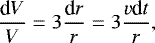
We used the canonical values for Type-1a explosions of Mej = 1.4 M⊙ and Eex = 1051 erg. The constant ambient density around the progenitor star then solely influences the evolution of the remnant. A value of n = 0.03 cm−3 leads to a forward-shock radius of Rfs = 2.2 pc at an age of 105 yr with a forward shock speed of vfs = 14 000 km s−1, which is in agreement with the extension of the bright X-ray ears measured with Chandra in 2008 (Reynolds et al. 2008). The extension of the reverse shock is Rrs = 1.85 pc at this age, which gives a ratio of  . The reverse shock speed is vrs = 11 000 km s−1 in the observer frame and 5650 km s−1 in the plasma frame. The time evolution of the shock properties is shown in Fig. 1. At this early stage of evolution the density immediately downstream of the reverse shock is still three times higher than the density downstream of the forward shock.
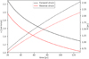 |
Fig. 1 Evolution of the speed (solid lines) and radius (dashed lines) of the forward and reverse shock in G1.9+0.3. |
3 Results
We constructed two different models for the particle acceleration in G1.9+0.3. The first assumes that all the radio and X-ray emission of the SNR is produced only at the forward shock under the assumption of Bohm-like diffusion in an amplified field. The second model takes the self-consistent amplification of turbulence at the forward shock into account and includes emission from the reverse shock.
3.1 One-shock model
Figure 2 shows the observed spectral energy distribution (SED) together with model curves representing the simulated emission from the remnant. Here we assumed Bohm-like diffusion in the downstream and in the upstream of the remnant up to a radius of 1.1 × Rsh. From 2 × Rsh we used the Galactic diffusion coefficient, and an exponential profile connects the two regimes in the intermediate range.
To simultaneously reproduce the flux of radio and X-ray emission, a very strong magnetic field, Bd ≈ 1.1 mG (Bu≈ 330 μG), is needed to produce sufficient synchrotron cooling to significantly modify the electron spectrum at the young age of the remnant.
To reproduce the observed synchrotron cutoff-energy, the diffusion coefficient must be increased by a factor of 30 compared to Bohm-like diffusion, implying ζ = 30 in Eq. (4), in agreement with Aharonian et al. (2017) who concluded that the diffusion upstream of G1.9+0.3 cannot be Bohm-like. Generally, Bohm-like diffusion is considered to be the most effective diffusion regime in SNRs, and the older remnants Cas A and RX J1713.4-3946 might well be within this regime (Zirakashvili & Aharonian 2010; Zirakashvili et al. 2014). A deviation towards a less efficient diffusion regime might indicate slow growth of magnetic turbulence at the largest scales.
Even though this model in principle explains the observed SED, the implied magnetic-field parameters are highly implausible. The downstream field corresponds to an energy density of
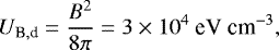 (18)
(18)
which is a sizable fraction of the energy density of the thermal plasma,
 (19)
(19)
The energy density of CRs in the immediate downstream region is
 (20)
(20)
and is considerably lower than that of the magnetic field.
Usually,just a few percent of the thermal energy of the plasma is assumed to be transformed to magnetic-field energy – otherwise the evolution of SNRs should considerably deviate from purely hydrodynamical predictions – whereas here an β ≈0.3 is needed. Themagnetic-field value obtained in this way is also a factor four higher than that derived assuming equipartition with CRs ≈ 270 μG (De Horta et al. 2014). In the case of equipartition, the energy density in CRs would be ≈ 1.8 × 10³eV cm−3, which is about 1.7% of the energy density of the thermal plasma.
The strong synchrotron cooling also affects the morphology of the remnant. In the emission profiles, the X-ray peak is always close behind the forward shock, as only recently accelerated electrons have sufficient energy to emit X-ray photons. Radio photons on the other hand can be emitted by all previously accelerated electrons in the downstream, leading to an offset of about 6% of the forward shock radius between the radio and the X-ray peaks in the emission profile. The observed separation between the peaks in the radio and the X-ray profiles is of the order 25% Rsh and hence incompatible with the one-shock scenario. None of the findings discussed above rely on a specific choice of turbulence modeling. They arise for both parametrized turbulence spectra and the solution of the transport equation for turbulence (cf. Eq. (5)). In the following, we explore the possibility of a two-shock scenario.
 |
Fig. 2 Model SED for the forward shock only in a uniform upstream medium. |
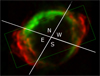 |
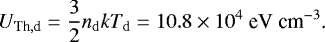
Fig. 3 Composite image of X-ray (red, Borkowski et al. 2017) and radio (green, Luken et al., in prep.) observations of G1.9+0.3, both from 2017. The green box marks the region from which we extracted the emission profiles. The bulk of the X-ray emission is concentrated in the E and W cones. The radio emission is brightest in the N and dimmer in the S. |
3.2 Two-shock model
As the simple one-shock scenario fell short of explaining the morphology of the emission of G1.9+0.3 and raised further questions related to the apparently nonBohm-like diffusion regime, we built a second model taking the reverse-shock of G1.9+0.3 into account.
Figure 3 illustrates the observed morphology of G1.9+0.3. We associate the X-ray emission with the forward shock because of its larger extension. The X-ray emission is concentrated in two cones in the east and west of the remnant, while the radio emission is more spherically symmetric. Possible reasons for the concentration of the emission in the cones are discussed in Sect. 3.2.1. The half-opening angle of the cones is ≈ 37.5° in projection, which gives a volume filling factor of about 20% for the X-ray bright and thus acceleration-efficient regions of the forward shock. As in a supersonic radial outflow there is little lateral transfer of energy or momentum, and we can treat the cones as sections of a spherically symmetric model. Hence, we scale all emission from the forward shock in our spherical symmetric model with the factor 20% to take into account the different radio and X-ray morphologies.
A proper description of shock acceleration requires that the transport equation for CRs be calculated on a grid that provides very high resolution at the shock where particles are injected. Hence we need to solve it separately for particles injected at the forward and reverse shock, respectively. The transport equation for magnetic turbulence, which includes the contributions of the streaming instability and turbulent dynamo action at the shocks, requires knowledge of the CR distribution for the streaming-instability term. As we must treat CRs accelerated at the forward and reverse shock separately, the full CR distribution is available only a posteriori. Typically, the forward shock provides the dominant contribution to the streaming instability, and hence we calculate the streaming contribution for particle acceleration at the forward shock. Large-scale MHD turbulence arising from a turbulent dynamo is added both downstream of the forward and downstream of the reverse shock.
The magnetic field immediately behind the forward shock is therefore not an independent parameter as in the one-shock model and is determined by the injectionparameter, ξ, and the conversion efficiency of the flow energy to magnetic field in the downstream of the shock, κ = 1.5%.
The streaming of particles from the forward shock only provides a very weak magnetic field at the reverse shock; its contributionto the total field strength is about 1%. For particles accelerated at the reverse shock we assume Bohm-like energy scaling for the diffusion coefficient for the particles accelerated at the reverse shock. The Larmor radius is calculated assuming that the total magnetic field near the reverse shock, which is obtained from the forward-shock calculation, can be interpreted as large-scale background magnetic field. This approximation appears justified for the low energy, and hence small Larmor radii, that particles accelerated at the reverse shock can attain. The scaling parameter for the diffusion coefficient, ζ in Eq. (4), with ζ = 5000, has the highest value that still permits a synchrotron cutoff higher than typical radio frequencies. The diffusion coefficient applied upstream of the reverse shock is about 1∕275 of the interstellar diffusion coefficient for particles of 1 GeV.
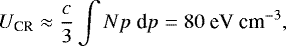
The particle spectra obtained from both shocks are then combined to calculate the emission from the remnant. The results for this model are shown in Fig. 4.
We use an injection parameter of ξ = 3.65 for the forward shock and a value of ξ = 3.5 for the reverse shock, which corresponds to a three-times-higher probability of injection there. The choice of different injection parameters is necessary to reproduce the measured flux ratio of the radio and the X-ray emission. Another way of reproducing the observed emission would be to use different values for the injection efficiency of post-shock turbulence, κ, at the two shocks. The higher injection efficiency at the reverse shock might be attributed to the lower shock speed there,as it is easier for particles to catch up to the shock there. We assume an electron-to-proton ratio1 of one eighth for both shocks and scale the emission of the forward-shock by one fifth to account for the observed X-ray morphology, as discussed above.
The peak magnetic-field value behind the forward shock is 180 μG, and we find about 120 μG downstreamof the reverse shock. The magnetic energy density downstream of both shocks is therefore only about 0.75% of the thermal energy density. Theother 0.75% of the thermal energy density that was converted into magnetic field is damped following cascading and converted back to thermal energy of the plasma. For both shocks, the ratio of CR pressure to shock ram pressure remains at ≈ 8.5%, justifying the test-particle assumption. About 70 μG from the 180 μG in the downstream is provided by the streaming of cosmic rays. This puts the ratio of δB∕B for the streaming instability at one, which is its supposed saturation level.
In this model the radio emission is dominated by the reverse shock, whereas the X-ray synchrotron emission is dominated by the forward shock. The high plasma density at the reverse shock during the current stage of remnant evolution naturally explains the high number density of accelerated particles there. The relatively large diffusion coefficient at the reverse shock is still sufficient to accelerate CRs to energies high enough to explain the bulk of the radio emission of G1.9+0.3. The exact value of the diffusion coefficient at the reverse shock is not important, as long as the maximum frequency of synchrotron emission does not fall below the observed radio frequencies and the CR-pressure does not exceed the test-particle limit. We illustrate the spatial distribution of high- and low-energetic electrons together with the magnetic-field structure in Fig. 5.
The magnetic-field profile we obtain strongly resembles the damped magnetic-field structure suggested by Pohl et al. (2005) and is shaped by the cascading of turbulence to smaller scales. Although no TeV-scale electrons are produced at the reverse shock, they can diffuse there in the damped turbulence, and their number density is still 6% of that at the forward shock.
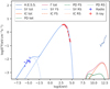 |
Fig. 4 Combined SED from the forward and reverse shocks. The letters FS (RS) denote emission from acceleration at the forward (reverse) shock, and SY, PD, and IC denote emission from synchrotron, pion decay, and inverse-Compton scattering, respectively. |
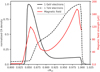 |
Fig. 5 Spatial distribution of the density of cosmic-ray electrons and the magnetic-field strength. |
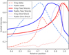 |
Fig. 6 Morphology of the remnant in X-rays and the radio band. The X-ray data are taken from Borkowski et al. (2017) and the radio-data are from Luken et al. (in prep.). The dashed lines indicate the intensity integrated in a rectangular region in the N-S direction covering the X-ray ears and projected onto the E-W axis. A similar method was applied to the theoretical data. |
3.2.1 Radio and X-ray morphology
The strong radio emission of electrons accelerated at the reverse shock significantly increases the separation between theradio and the X-ray peak in the emission profiles. A comparison is shown in Fig. 6. The observed separation of the two peaks is about 25% of the forward-shock radius, and accounting for two shocks increases the peak-separation in the model from 6.5% in the one-shock scenario to about 15% Rsh of the shock radius. The two-shock scenario may also explain the different morphology of the X-ray and the radio emission. The bipolar structure in X-rays is similar to the emission structure in SN1006 and may reflect the orientation of the local magnetic field by either limiting the acceleration efficiency at a perpendicular shock or limiting the injection efficiency (Völk et al. 2003). If so, the reverse shock would be unaffected by the magnetic field of the ISM. The magnetic-field structure expected in the unshocked ejecta would favor similar injection conditions over the entire reverse-shock surface.
The observed azimuthal variation in the intensity around the reverse-shock region can in this scenario still be attributed to a density gradient in the ISM with a higher density towards the north or alternatively an anisotropic explosion as indicated by the inhomogeneous distribution of heavier elements in the ejecta (Borkowski et al. 2013). Both scenarios would lower (enhance) the expansion speed of the remnant towards the north (south) and lead to a higher (lower) density at the reverse shock. Thus the brightness difference between north and south would be attributed to the presence of more or less electrons that can be accelerated.
There are several potential explanations for why in our model the intensity peaks in the radio and the X-ray band are closer together by 5% Rsh than they are observed to be. First, if the supernova explosion was anisotropic, our assumed ejecta distribution could be inappropriate or not be independent of direction. If the ejecta distribution were shallower, the position of the reverse shock would be further inward. A lower ejecta mass in one direction of the supernova expansion could result in faster deceleration of the forward shock with the consequence that the separation between forward and reverse shocks would be larger. Second, an asymmetric explosion or expansion in a inhomogeneous medium leads to a displacement of the geometric center of the remnantfrom the explosion site, and hence to a false estimate of the shock radius, yielding a different shock radius in each direction from the center of the explosion. It follows that the relative separation of the two shocks measured from the geometrical center of the explosion will be different in all directions. Modeling of an anisotropic explosion is beyond the scope of this paper, and we tried to minimize the impact of this distortion by averaging the E-W profile in the N-S direction, but as the exact geometry of the explosion is unknown, there might still be a remaining effect. Third, as the emission of the forward and the reverse shock is decoupled, there is no reason why the effects determining the morphology of the X-ray – the ambient magnetic-field structure – and the radio emission – the density gradient or the structure of the explosion – should be aligned. If they are not aligned, then projection effects might result in a higher separation between the peaks of the X-ray and the radio emission. If, for example, the X-ray emission is aligned with the plane of the sky, then a tilt of the density gradient by 25° is enough to shift the apparent position of the reverse shock from 84% of the forward shock radius to 75%.
It is important to note that the morphological difference between radio and X-ray emission makes G1.9+0.3 the first SNR for which nonthermal emission can be clearly attributed to the reverse shock. Nonthermal emission from the reverse shock has been discussed for RX J1713.7-3946 (Zirakashvili & Aharonian 2010) and Cas A (Zirakashvili et al. 2014; Helder & Vink 2008) as well but on a much more tenuous basis than in the case of G1.9+0.3. The model of Zirakashvili & Aharonian (2010) for RX J1713.7-3946 requires a sizable nonthermal emission from the reverse shock only for a hadronic model of the gamma-ray emission of the remnant. If the gamma-ray emission is leptonic, an enhanced magnetic field towards the Rayleigh–Taylor unstable contact discontinuity can explain the observed radio and X-ray morphology of the remnant. However, the low-density environment around RX J1713.7-3946 makes a leptonic scenario more likely unless a clumpy medium around the remnant provides enough target material (Inoue et al. 2012) and there is a way to avoid emitting a detectable flux of X-rays (Federici et al. 2015). For Cas A, Zirakashvili et al. (2014) argue that a contribution from particles accelerated at the reverse shock is possible, but the radio morphology might also be attributed to an enhanced magnetic field towards the contact discontinuity. Although an association of X-ray emission with the reverse shock was suggested by earlier data (Helder & Vink 2008), the hard X-ray emission from Cas A appears to come from knots and filaments that are not well correlated with the reverse shock (Grefenstette et al. 2015). However, these knots appear to be moving inwards far faster than expected for the reverse shock of Cas-A given its stage of evolution (Sato et al. 2018).
The lack of X-ray emission from the position of the radio shell of G1.9+0.3 is not in line with an enhanced magnetic field near the contact discontinuity, because high-energy electrons accelerated at the forward shock should be able to diffuse there and produce intense X-ray emission which is not observed.
3.2.2 Radio brightening
The large dataset collected by MOST shows a brightening of the total radio flux at 843 MHz at a rate of  % yr−1 (Murphy et al. 2008). This brightening can be attributed either to an increase of the magnetic field strength or to an increase of the number of radiating electrons.
For a type-Ia supernova the relative increase in the number of radiating particles can be estimated as
 (21)
(21)
resulting in 1.9% yr−1 for the forward shock and 1.6% yr−1 for the reverse shock.
In our simulations we obtain a value of 0.75% yr−1, which is compatible within 2σ with the observed rate, but lower than the brightening expected for a constant magnetic-field strength and a constant upstream density. Figure 7 shows the simulated and measured time evolution of the radio flux. However, the density upstream of the reverse shock is decreasing with a rate of ≈ 0.7% yr−1 which reduces the expected analytic brightening rate to ≈ 0.9% yr−1.
Alternatively, if the evolution of the number of electrons is well known, the observed brightening rate can provide a measurement of the change of the magnetic-field strength in the remnant. The observed value of about 1.2% yr−1 would be reproduced if the magnetic-field strength increased by 0.15% yr−1. At this time, the uncertainty in the rate of radio brightening is too large to establish a nonzero evolution of the magnetic-field strength.
None of the observed properties of G1.9+0.3, except the radio brightening, depend on our parametrization of the post-shock turbulence. A significant fraction of the magnetic field is assumed to arise from MHD instabilities at the shock. If we coupled the injection of turbulence dynamically to the energy density in the post-shock flow, the magnetic field would decrease over time, because the shock velocity decreases at both shocks and so does the plasma density at the reverse shock. Taking this at face value, the radio brightness of G1.9+0.3 would decrease by 0.23% yr−1. The data suggest otherwise, and so we implemented a fixed injection of large-scale turbulence, leading to an almost constant magnetic field. In reality, part of the MHD turbulence may be triggered by cosmic-ray interactions in the precursor that need time to build up (Beresnyak et al. 2009; del Valle et al. 2016), and the efficiency of MHD-turbulence injection may have a nontrivial time profile.
As the X-ray emission originates at the forward shock, we expect its brightening rate to be different from that of the radio emission. Our model yields a brightening rate of 1.5% yr−1, which is slightly below the analytic value we expect for a constant magnetic field and is close to the observed values of 1.9 ± 0.4% yr−1 (Borkowski et al. 2014) and 1.3 ± 0.8% yr−1 (Borkowski et al. 2017).
We did not account for an amplification of magnetic field at the reverse shock through, for example, processes driven by accelerated cosmic rays or Rayleigh–Taylor and Helmholtz instabilities that will develop at the contact discontinuity. This would provide additional magnetic field at or close to the reverse shock and allow to fit the SED with fewer particles injected at the reverse shock. Likewise, the structure of the medium encountered by the shock is decisive for the development of post-shock turbulence. For example, an inhomogeneous distribution of the ejecta may increase the conversion efficiency of flow energy to magnetic field at the reverse shock. Our coupling of the energy density transferred to post-shock turbulence to the energy density of the flow is likely an over-simplified parametrization of the physics at play.
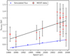 |
Fig. 7 Time evolution of the radio flux at 843 MHz. |
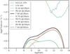 |
Fig. 8 Gamma-ray spectrum from G1.9+0.3 in 2007 (gray line) and 2032 (black line). The letters IC and PD denote emission from inverse-Compton scattering and pion decay, respectively, while FS (RS) denotes emission from the forward (reverse) shock. |
3.2.3 Prospects for CTA
The TeV-band gamma-ray emission from G1.9+0.3 is dominated by inverse Compton scattering of CMB and IR photons off high-energy electrons accelerated at the forward shock. We approximated the IR-radiation field from Porter et al. (2006) at the location of G1.9+0.3 with a gray-body distribution with temperature TIR = 55 K and energy density UIR = 1.5 eV cm−3. Figure 8 shows that our predictions for the gamma-ray flux are in close agreement with the H.E.S.S upper limits and are about six times below the design sensitivity of CTA south for 50 h of observations.
Given that G1.9+0.3 is located within the survey field of the Galactic center with more than 500 h of observations planned for that region, a 3σ detection of the signal from G1.9+0.3 could still be possible in the event of future improvements in sensitivity over the original design specifications.
We expect the gamma-ray flux to increase by about 25% in the epoch between 2007 and 2032. The gamma-ray luminosity of G1.9+0.3 above 1 TeV would be ≈ 1.0 ⋅ 1032 erg s−1, which is well within the range found by H.E.S.S. in their SNR population study (H.E.S.S. Collaboration 2018).
4 Conclusions
We modeledthe broadband nonthermal emission from the SNR G1.9+0.3 with a view to analyzing the observed SED, the morphology,and the brightening rate at radio frequencies, and to elucidate the prospects for detecting the remnant with CTA. For that purpose we solved the transport equations for cosmic rays and Alfvénic turbulence together with the standard gas-dynamical equations, and we subsequently calculated the emission spectra from the forward and the reverse shock under the assumption of spherical symmetry.
We showed that a scenario involving only the forward shock needs a very strong magnetic field in order to explain the SED of the remnantand falls short of explaining the separation between the peaks of radio and X-ray emission. The required magnetic-field strength in this scenario is well above the equipartition value and implies the same energy density in the magnetic field and in the thermal plasma, which is very unlikely.
Allowing for electron acceleration at the reverse shock reproduces the SED with lower magnetic-field strength and decouples the X-ray and radio emission, the former arising from multi-TeV electrons accelerated at the forward shock and the latter produced bythe large number of lower-energy electrons energized at the reverse shock. While the bipolar X-ray morphology might be the result of a variation in acceleration efficiency due to the magnetic-field structure, the radio morphology would be unaffected by this. A density gradient in the ambient medium towards the north or an asymmetric explosion is sufficient to explain the radio N-S asymmetry. It would also account for the difference in expansion velocity measured between X-ray and radio features in the E-W direction and better reproduce the separation between the radio and X-ray peaks.
The observed radio brightening rate is consistent with a magnetic field that is constant over time. Our model predicts a brightening rate of 0.75% yr−1, compatible within 2σ with the observed  % yr−1.
The limited time available to drive large-scale turbulence in the upstream region naturally causes super-Bohmian diffusion and hence an acceleration efficiency well below that expected for Bohm diffusion. The maximum energy of particles is below 100 TeV, and so G1.9+0.3 is not a PeVatron.
We further evaluated the prospects of detecting G1.9+0.3 with the CTA observatory. Our model predicts a brightening of G1.9+0.3 by ≈ 25% between 2007 and 2032 and a gamma-ray flux that is approximately six times below the design sensitivity of CTA for 50 h of observations. Essentially all of the TeV-scale gamma-ray flux is produced by particles accelerated at the forward shock, and the majority comes from inverse-Compton scattering. Pion-decay radiation contributes about 20% of the flux.
Our model indicates that G1.9+0.3 is the first SNR with detected nonthermal emission that can be clearly attributed to the reverse shock.
References
- Aharonian, F., Sun, X.-n., & Yang, R.-z. 2017, A&A, 603, A7 [NASA ADS] [CrossRef] [EDP Sciences] [Google Scholar]
- Bell, A. R. 1978, MNRAS, 182, 147 [NASA ADS] [CrossRef] [Google Scholar]
- Bell, A. R. 2004, MNRAS, 353, 550 [Google Scholar]
- Bell, A. R., Schure, K. M., Reville, B., & Giacinti, G. 2013, MNRAS, 431, 415 [NASA ADS] [CrossRef] [Google Scholar]
- Beresnyak, A., Jones, T. W., & Lazarian, A. 2009, ApJ, 707, 1541 [NASA ADS] [CrossRef] [Google Scholar]
- Blasi, P., Gabici, S., & Vannoni, G. 2005, MNRAS, 361, 907 [NASA ADS] [CrossRef] [Google Scholar]
- Bohdan, A., Niemiec, J., Kobzar, O., & Pohl, M. 2017, ApJ, 847, 71 [NASA ADS] [CrossRef] [Google Scholar]
- Borkowski, K. J., Reynolds, S. P., Hwang, U., et al. 2013, ApJ, 771, L9 [NASA ADS] [CrossRef] [Google Scholar]
- Borkowski, K. J., Reynolds, S. P., Green, D. A., et al. 2014, ApJ, 790, L18 [NASA ADS] [CrossRef] [Google Scholar]
- Borkowski, K. J., Gwynne, P., Reynolds, S. P., et al. 2017, ApJ, 837, L7 [NASA ADS] [CrossRef] [Google Scholar]
- Brose, R., Telezhinsky, I., & Pohl, M. 2016, A&A, 593, A20 [NASA ADS] [CrossRef] [EDP Sciences] [Google Scholar]
- Cherenkov Telescope Array Consortium 2017, Science with the Cherenkov Telescope Array (Singapore: World Scientific) [Google Scholar]
- De Horta, A. Y., Filipovic, M. D., Crawford, E. J., et al. 2014, Serb. Astron. J., 189, 41 [NASA ADS] [Google Scholar]
- del Valle, M. V., Lazarian, A., & Santos-Lima, R. 2016, MNRAS, 458, 1645 [NASA ADS] [CrossRef] [Google Scholar]
- Dwarkadas, V.V., & Chevalier, R. A. 1998, ApJ, 497, 807 [NASA ADS] [CrossRef] [Google Scholar]
- Federici, S., Pohl, M., Telezhinsky, I., Wilhelm, A., & Dwarkadas, V. V. 2015, A&A, 577, A12 [NASA ADS] [CrossRef] [EDP Sciences] [Google Scholar]
- Fraschetti, F. 2014, Nucl. Instrum. Methods Phys. Res. A, 742, 169 [NASA ADS] [CrossRef] [Google Scholar]
- Green, D. A., & Gull, S. F. 1984, Nature, 312, 527 [NASA ADS] [CrossRef] [Google Scholar]
- Green, D. A., Reynolds, S. P., Borkowski, K. J., et al. 2008, MNRAS, 387, L54 [NASA ADS] [CrossRef] [Google Scholar]
- Grefenstette, B. W., Reynolds, S. P., Harrison, F. A., et al. 2015, ApJ, 802, 15 [NASA ADS] [CrossRef] [Google Scholar]
- Guyer, J. E., Wheeler, D., & Warren, J. A. 2009, Comput. Sci. Eng., 11, 6 [CrossRef] [Google Scholar]
- Helder, E. A., & Vink, J. 2008, ApJ, 686, 1094 [NASA ADS] [CrossRef] [Google Scholar]
- H.E.S.S. Collaboration (Abramowski, A., et al.) 2014, MNRAS, 441, 790 [NASA ADS] [CrossRef] [Google Scholar]
- H.E.S.S. Collaboration (Abdalla, H., et al.) 2018, A&A, 612, A3 [NASA ADS] [CrossRef] [EDP Sciences] [Google Scholar]
- Inoue, T., Yamazaki, R., Inutsuka, S.-i., & Fukui, Y. 2012, ApJ, 744, 71 [NASA ADS] [CrossRef] [Google Scholar]
- Kang, H., & Ryu, D. 2010, ApJ, 721, 886 [NASA ADS] [CrossRef] [Google Scholar]
- Lucek, S. G., & Bell, A. R. 2000, MNRAS, 314, 65 [NASA ADS] [CrossRef] [Google Scholar]
- Matsumoto, Y., Amano, T., & Hoshino, M. 2012, ApJ, 755, 109 [NASA ADS] [CrossRef] [Google Scholar]
- Matsumoto, Y., Amano, T., Kato, T. N., & Hoshino, M. 2017, Phys. Rev. Lett., 119, 105101 [CrossRef] [Google Scholar]
- Mignone, A., Bodo, G., Massaglia, S., et al. 2007, ApJS, 170, 228 [Google Scholar]
- Murphy, T., Gaensler, B. M., & Chatterjee, S. 2008, MNRAS, 389, L23 [NASA ADS] [CrossRef] [Google Scholar]
- Pavlović, M. Z. 2017, MNRAS, 468, 1616 [NASA ADS] [Google Scholar]
- Pohl, M. 1993, A&A, 270, 91 [NASA ADS] [CrossRef] [Google Scholar]
- Pohl, M., Yan, H., & Lazarian, A. 2005, ApJ, 626, L101 [NASA ADS] [CrossRef] [Google Scholar]
- Porter, T. A., Moskalenko, I. V., & Strong, A. W. 2006, ApJ, 648, L29 [NASA ADS] [CrossRef] [Google Scholar]
- Reynolds, S. P., Borkowski, K. J., Green, D. A., et al. 2008, ApJ, 680, L41 [NASA ADS] [CrossRef] [Google Scholar]
- Sato, T., Katsuda, S., Morii, M., et al. 2018, ApJ, 853, 46 [NASA ADS] [CrossRef] [Google Scholar]
- Schlickeiser, R. 2002, Cosmic Ray Astrophysics (Berlin: Springer Science & Business Media) [CrossRef] [Google Scholar]
- Skilling, J. 1975, MNRAS, 172, 557 [NASA ADS] [CrossRef] [Google Scholar]
- Telezhinsky, I., Dwarkadas, V. V., & Pohl, M. 2012a, Astropart. Phys, 35, 300 [NASA ADS] [CrossRef] [Google Scholar]
- Telezhinsky, I., Dwarkadas, V. V., & Pohl, M. 2012b, A&A, 541, A153 [NASA ADS] [CrossRef] [EDP Sciences] [Google Scholar]
- Telezhinsky, I., Dwarkadas, V. V., & Pohl, M. 2013, A&A, 552, A102 [NASA ADS] [CrossRef] [EDP Sciences] [Google Scholar]
- Threlfall, J., McClements, K. G., & De Moortel, I. 2011, A&A, 525, A155 [NASA ADS] [CrossRef] [EDP Sciences] [Google Scholar]
- Trotta, R., Jóhannesson, G., Moskalenko, I. V., et al. 2011, ApJ, 729, 106 [NASA ADS] [CrossRef] [Google Scholar]
- Völk, H. J., Berezhko, E. G., & Ksenofontov, L. T. 2003, A&A, 409, 563 [NASA ADS] [CrossRef] [EDP Sciences] [Google Scholar]
- Wentzel, D. G. 1974, ARA&A, 12, 71 [NASA ADS] [CrossRef] [Google Scholar]
- Zhou, Y., & Matthaeus, W. H. 1990, J. Geophys. Res., 95, 14881 [NASA ADS] [CrossRef] [Google Scholar]
- Zirakashvili, V. N., & Aharonian, F. A. 2010, ApJ, 708, 965 [NASA ADS] [CrossRef] [Google Scholar]
- Zirakashvili, V. N., Aharonian, F. A., Yang, R., Oña-Wilhelmi, E., & Tuffs, R. J. 2014, ApJ, 785, 130 [NASA ADS] [CrossRef] [Google Scholar]

All Figures
|
Fig. 1 Evolution of the speed (solid lines) and radius (dashed lines) of the forward and reverse shock in G1.9+0.3. |
| In the text | |
|
Fig. 2 Model SED for the forward shock only in a uniform upstream medium. |
| In the text | |
|
Fig. 3 Composite image of X-ray (red, Borkowski et al. 2017) and radio (green, Luken et al., in prep.) observations of G1.9+0.3, both from 2017. The green box marks the region from which we extracted the emission profiles. The bulk of the X-ray emission is concentrated in the E and W cones. The radio emission is brightest in the N and dimmer in the S. |
| In the text | |
|
Fig. 4 Combined SED from the forward and reverse shocks. The letters FS (RS) denote emission from acceleration at the forward (reverse) shock, and SY, PD, and IC denote emission from synchrotron, pion decay, and inverse-Compton scattering, respectively. |
| In the text | |
|
Fig. 5 Spatial distribution of the density of cosmic-ray electrons and the magnetic-field strength. |
| In the text | |
|
Fig. 6 Morphology of the remnant in X-rays and the radio band. The X-ray data are taken from Borkowski et al. (2017) and the radio-data are from Luken et al. (in prep.). The dashed lines indicate the intensity integrated in a rectangular region in the N-S direction covering the X-ray ears and projected onto the E-W axis. A similar method was applied to the theoretical data. |
| In the text | |
|
Fig. 7 Time evolution of the radio flux at 843 MHz. |
| In the text | |
|
Fig. 8 Gamma-ray spectrum from G1.9+0.3 in 2007 (gray line) and 2032 (black line). The letters IC and PD denote emission from inverse-Compton scattering and pion decay, respectively, while FS (RS) denotes emission from the forward (reverse) shock. |
| In the text | |
Current usage metrics show cumulative count of Article Views (full-text article views including HTML views, PDF and ePub downloads, according to the available data) and Abstracts Views on Vision4Press platform.
Data correspond to usage on the plateform after 2015. The current usage metrics is available 48-96 hours after online publication and is updated daily on week days.
Initial download of the metrics may take a while.