| Issue |
A&A
Volume 626, June 2019
|
|
|---|---|---|
| Article Number | A84 | |
| Number of page(s) | 20 | |
| Section | Interstellar and circumstellar matter | |
| DOI | https://doi.org/10.1051/0004-6361/201834998 | |
| Published online | 18 June 2019 | |
Analysis and test of the central-blue-spot infall hallmark
1
Departament de Física Quàntica i Astrofísica, Institut de Ciències del Cosmos, Universitat de Barcelona, IEEC-UB,
Martí i Franquès 1,
08028
Barcelona,
Spain
e-mail: robert.estalella@ub.edu
2
Instituto de Astrofísica de Andalucía, CSIC,
Glorieta de la Astronomía, s/n,
18008
Granada,
Spain
Received:
30
December
2018
Accepted:
13
April
2019
Aims. The infall of material onto a protostar, in the case of optically thick line emission, produces an asymmetry in the blue- and red-wing line emissions. For an angularly resolved emission, this translates in a blue central spot in the first-order moment (intensity weighted velocity) map.
Methods. An analytical expression for the first-order moment intensity as a function of the projected distance was derived, for the cases of infinite and finite infall radius. The effect of a finite angular resolution, which requires the numerical convolution with the beam, was also studied.
Results. This method was applied to existing data of several star-forming regions, namely G31.41+0.31 HMC, B335, and LDN 1287, obtaining good fits to the first-order moment intensity maps, and deriving values of the central masses onto which the infall is taking place (G31.41+0.31 HMC: 70–120 M⊙; B335: 0.1 M⊙; Guitar Core of LDN 1287: 4.8 M⊙). The central-blue-spot infall hallmark appears to be a robust and reliable indicator of infall.
Key words: ISM: jets and outflows / ISM: individual objects: G31.41+0.31 HMC / ISM: individual objects: B335 / stars: formation / ISM: individual objects: LDN 1287
© ESO 2019
1 Introduction
The early phases of star formation are characterized by infall motions of ambient material onto a central protostellar object. However, obtaining unequivocal observational evidence for these motions constitutes a long-standing problem. Rotation, infall and outflow motions can be present simultaneously in the early phases of star formation, and may produce similar observational features in the line profiles, making an unambiguous interpretation of the observations difficult.
The most common method used so far to search for evidence of infall is based on the so-called “blue asymmetry”. This signature consists in the appearance of two peaks in the spectral line profiles, with the blueshifted peak stronger than the redshifted peak (e.g., Zhou et al. 1994; Klaassen & Wilson 2007; Wu et al. 2007). However, the effect of protostellar infall on molecular line profiles cannot be easily isolated from those of other dynamical processes, resulting in ambiguities (e.g., Purcell et al. 2006; Szymczak et al. 2007). Inverse P-Cygni profiles, which consist in the detection of absorption at redshifted velocities against a bright background continuum source, have been observed in molecular lines against a bright background HII region (e.g., Keto et al. 1987; Zhang et al. 1998) or against the bright dust continuum emission of the hot protostellar core itself (e.g., Di Francesco et al. 2001; Girart et al. 2009), and have been interpreted as infall motions of the surrounding envelope. Nevertheless, it uniquely indicates that foreground matter is moving toward a hotter source, no matter how or if it is indeed gravitationally bound. See Mayen-Gijon et al. (2014) and Mayen-Gijon (2015) for a thorough review of infall signatures.
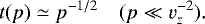
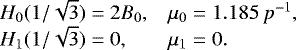
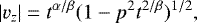
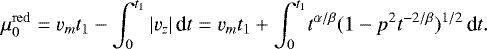
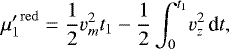
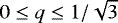
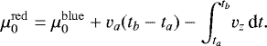
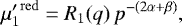
Anglada et al. (1991) introduce a more complete signature, the “3D spectral imaging infall signature”, which is based on the spatial distribution of the line emission intensity in the images as a function of the line-of-sight (LOS) velocity (i.e., the channel maps). This signature, appropriate for angularly resolved sources, results as an extension of the formalism initially developed by Anglada et al. (1987) for the study of an angularly unresolved infalling core. These signatures are focused on relatively high velocities, in order to avoid confusion with emission from the ambient cloud at low velocities. With the assumption of gravitational infall motions dominating the kinematics over turbulent and thermal motions, and spherical symmetry with an infall velocity increasing inwards, it can be shown that the points of the infalling core with the same LOS velocity form closed surfaces. The equal-LOS-velocity surfaces are a nested set of surfaces with the same shape, decreasing in size with increasing absolute value of the LOS velocity, and converging to the position of the core center (see Fig. 1).
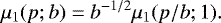
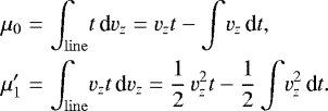
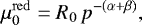
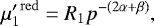
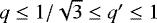
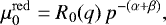
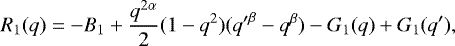
Because the equal-LOS-velocity surfaces are closed surfaces, a given LOS, in general, intersects the same surface twice. However, if the opacity is high enough, only a narrow layer at the front side of the equal-LOS-velocity surface is observable. Hence, the intensity map at a given LOS velocity is an image of the excitation temperature distribution in the side of the equal-LOS-velocity surface facing the observer (thick lines in Fig. 1), while the emission from the rear side remains hidden (thin lines in Fig. 1). Thus, the shapes of the blueshifted and redshifted emitting regions1 are different. Since the temperature increases inwards, the integrated blueshifted emission comes from a region closer, on average, to the central protostar (and, therefore, hotter) than the corresponding redshifted emission, resulting in asymmetric line profiles, with the blueshifted wing stronger than the redshifted wing (Anglada et al. 1987). The difference is still more remarkable for a pair of blueshifted–redshifted channel maps. Assuming that the maps are centered on the position of the protostar, for the redshifted channel the intensity is slightly lower at the center of the map than at the edges, because toward the center the side of the equal-LOS-velocity surface facing the observer is slightly farther away from the center of the core and thus, colder than the rest of the surface. For the blueshifted channel, the intensity increases sharply toward the center of the image since this emission comes from a region very close to the center of the core and, therefore, very hot (see Fig. 2). In addition, since the size of the equal-LOS-velocity surfaces decreases with increasing absolute value of the LOS velocity, the emission becomes more compact for increasing absolute value of the LOS velocity (see Fig. 2).
This behavior of the intensity maps for redshifted and blueshifted LOS velocities produces a characteristic signature in the intensity-weighted mean velocity (first-order moment) map, which was pointed out by Mayen-Gijon et al. (2014), in other words, that the central region of the first-order map appears blueshifted because of the higher weight of the strong blueshifted emission. Additionally, the integrated intensity, (zeroth-order moment) peaks toward the central position. At larger distances from the center, the integrated intensity decreases, the blue andredshifted intensities become similar, and the intensity-weighted mean velocity approaches the systemic velocity of the cloud. Therefore, the first-order moment of an infalling envelope is characterized by a compact spot of blueshifted emission toward the position of the zeroth-ordermoment peak. This infall hallmark is designated as the “central blue spot” (Mayen-Gijon et al. 2014; Mayen-Gijon 2015). One of the advantages of the central-blue-spot infall hallmark is that its detection does not require a beforehand knowledge of the systemic velocity of the cloud. An accurate knowledge of the systemic velocity is critical in searching for infall through the analysis of asymmetries in the line profiles.
Mayen-Gijon et al. (2014) and Mayen-Gijon (2015) identify both the 3D spectral imaging infall signature and the central-blue-spot hallmark in high-angular resolution maps of the emission of several NH3 transitions toward G31.41+0.31 HMC, and compare the observed emission with the predictions of a spherically symmetric model with full transport of radiation calculation (Osorio et al. 2009).
If there is rotation, the LOS velocity has contributions from both the infalling velocity and the rotation velocity. Mayen-Gijon et al. (2014) and Mayen-Gijon (2015), in the analysis of the NH3 data of G31.41+0.31 HMC, discuss qualitatively how rotation affects the channel maps of an infalling core. These authors find that the radial intensity profile of the image for a given LOS-velocity channel is stretched toward the side where rotation has the same sign than the channel velocity, and it is shrunk on the opposite side. Nevertheless, as in the non-rotating case, the images in blue-shifted channels present a centrally peaked intensity distribution, while in the red-shifted channels they present a flatter intensity distribution. Thus, the rotation signature makes the spatial intensity profiles asymmetric with respect to the central position but it does not mask the 3D spectral imaging infall signature of Anglada et al. (1991).
Regarding the first-order moment map, Mayen-Gijon (2015) explores how the central-blue-spot hallmark of an infalling core is modified by the presence of rotation. He finds that rotation makes the central-blue-spot even bluer and moves it off the center toward the half of the core where rotation tends to shift velocities to the blue. Additionally, a dimmer red spot appears symmetrically located on the opposite side of the rotation axis.
In the present paper we studied quantitatively the central-blue-spot infall hallmark, restricted to the spherically symmetric case without rotation, taking as a basis the work of Anglada et al. (1987, 1991). Using the same assumptions than in these papers, we derived analytical expressions for the intensity profiles (Sect. 2), the line profiles (Sect. 3), and the first-order moment of the intensity profile (Sect. 4) as functions of the angular distance from the center. This was done for the case of an infinite infall radius, without considering the effect of a finite angular resolution. The details of the derivation for arbitrary values of the power-law indices are given in Appendix A. The effect of a finite spectral resolution is addressed in Sect. 4.2 and Appendix C, while the effect of a finite angular resolution is studied in Sect. 4.3 and Appendix D. The case of a finite infall radius is presented in Sect. 5, where an analytical expression for the first-order moment is obtained. The details of the derivation for arbitrary values of the power-law indices are given in Appendix B. The transformation between reduced units and practical units is described in Sect. 6. The results are applied to several cases (G31.41+0.31 HMC, B335, LDN 1287) in Sect. 7, with the analysis of pre-existing data that show the central-blue-spot infall hallmark. Finally, the conclusions are given in Sect. 8.
2 Intensity profile
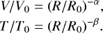
Based on Anglada et al. (1987, 1991), we are assuming an infalling molecular gas core, with infall velocity and temperature given by power laws of the radius (Eq. (1) of Anglada et al. 1987),
 (1)
(1)
where R0 is a reference radius. The power-law indices of the infall velocity and temperature are taken with a value α = β = 1∕2, that is, free-fall velocity, and optically thin dust heating from a central protostar, which are characteristic of the main accretion phase in the Larson collapse model (Larson 1972) or in the Shu (1977) inside-out collapse model. In the Appendices A and B the case of arbitrary values of the power-law indices is developed.
Let the coordinate z be along the line of sight, positive outwards from the observer, and p the impact parameter, that is, the distance to the center projected on the plane of the sky (see Fig. 1). All coordinates are lengths in units of R0, so that the distance to the center in units of R0 is
 (2)
(2)
Let us define the reduced line-of-sight (LOS) velocity and temperature
 (3)
(3)
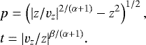
Equations (9) and (10) of Anglada et al. (1991) can be expressed in reduced variables as
![\begin{eqnarray*}&& \hspace*{-6pt} p = \left[ |z/v_z|^{4/3} - z^2\right]^{1/2}, \nonumber\\ &&\hspace*{-6pt} t = |v_z/z|^{1/3}. \end{eqnarray*}](/articles/aa/full_html/2019/06/aa34998-18/aa34998-18-eq4.png) (4)
(4)
For a given |vz| Eq. (4) gives the parametric equation (with z as parameter) of the intensity profile, t(p). We are assuming that the intensity observed at a given LOS velocity comes from the part of the equal-LOS-velocity surface facing the observer. Thus, the blue-wing intensity profile (vz < 0) is obtained for 0 < z < zm, while the red-wing intensity profile (vz > 0) is obtained for − z* < z < −zm, where zm is the value of z for which p is maximum for a given vz, p = pm (see Fig. 1), and z* is the maximum value of z for a given equal-LOS-velocity surface. The value of z* is obtained from Eq. (4) for p = 0, z* = |vz|−2. The value of zm can be obtained from the derivative of p(z) given in Eq. (4), and the values obtained for zm and pm are
 (5)
(5)
The ratio zm∕pm is independentof vz,  , meaning that the points (zm, pm) are aligned along a straight line passing through the center, with a slope of
  (see Fig. 1).
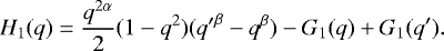
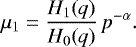
For any LOS-velocity the emission is confined inside a projected distance p < pm. For blueshifted LOS-velocities (vz < 0) the intensity increases sharply for small projected distances p, while for redshifted LOS-velocity (vz > 0) the intensityis almost flat up to pm (see Figs. 3 and 4). This can be seen in Fig. 2, where we show the intensity maps, for LOS pairs of positive and negative LOS velocities.
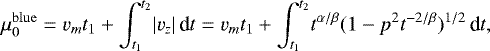
For the maximum projected distance pm the red-wing intensity is maximum, and equal to the minimum blue-wing intensity (see Fig. 3),
 (6)
(6)
The blue wing intensity for small projected distances is very high, and for the adimensional temperature and LOS velocity t ≫ vz we obtain the asymptotic behavior (see Fig. 3)
 (7)
(7)
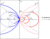 |
Fig. 1 Intersection of the surfaces of equal line-of-sight (LOS) velocity, vz, for a collapsing protostellar core, with the plane (p, z) (see Sect. 2). The LOS-velocities are different pairs of negative and positive velocities (vz = ±2−1∕2, ±1, ±21∕2, ±2). The blue lines are the contours for vz < 0, and the red lines for vz > 0. The observer, located to the right, at p = 0, z = −∞, sees the emission coming from the part of the surfaces of equal LOS-velocity facing the observer, traced with thick lines. The dashed lines indicate the position of (zm, pm) for each contour, where pm is the maximum value of p, and zm the corresponding value of z. The square frame is drawn at p = ±1, z = ±1. |
 |
Fig. 2 Intensity maps for pairs of LOS-velocities, Vz = ±0.8 km s−1 (top), ± 1.1 km s−1 (middle), and ± 1.4 km s−1 (bottom), calculated for a a mass M* = 1 M⊙, a distance of 140 pc, and a beam of 0.′′1. The axes are position offsets labeled in arcsec. The intensity scale is the same for all maps. We note the sharp peak at the center of the blueshifted LOS-velocity maps (left), and the flat, slightly concave shape of the redshifted LOS-velocity maps (right), and the more compact emission for high values |Vz | (bottom) than for low values of |Vz| (top). |
3 Line profile
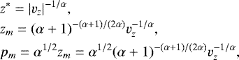
In order to calculate the first-order moment intensity, we need to obtain the line intensity for any value of p. Thus, we want to derive the intensity and LOS velocity for a given projected distance p. From Eq. (4) we can obtain easily the LOS velocity and temperature as functions of p and z,
![\begin{eqnarray}&&\hspace*{-6pt} v_z = \frac{-z}{(p^2+z^2)^{3/4}}, \nonumber\\[3pt] &&\hspace*{-6pt} t = \frac{1}{(p^2+z^2)^{1/4}}. \end{eqnarray}](/articles/aa/full_html/2019/06/aa34998-18/aa34998-18-eq10.png) (8)
(8)
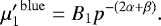
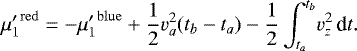
These equations can be interpreted as the parametric equation (with z as parameter) of the line profile t(vz) for a given projected distance p (see Figs. 5 and 6).
The line of sight with a given p intersects equal-LOS-velocity surfaces of decreasing size, down to that corresponding to pm = p. For this equal-LOS-velocity surface, the blueshifted velocity is minimum (maximum absolute value) and the redshifted velocity is maximum (see Fig. 1). This occurs at the points with coordinate  .
.
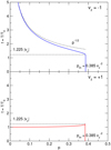 |
Fig. 3 Intensity profiles t(p) for vz = −1 (top panel, blue) and vz = +1 (bottom panel, red). The different dashed lines indicate the blue and red wing temperature at the maximum value of p, p = pm, and the blue wing asymptotic behavior for p ≪ 1. |
3.1 Blue wing
The observable intensity at blueshifted velocities (vz < 0) is obtained for 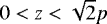 . For a given value of p, the minimum blueshifted intensity
  and minimum velocity
  (maximum absolute value) are obtainedat the point
 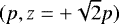 ,
,
![\begin{eqnarray*}&&\hspace*{-6pt} t^{\mathrm{blue}}_{\mathrm{min}} \equiv t_1 = 3^{-1/4}\,p^{-1/2}= 0.760\,p^{-1/2}, \nonumber\\[3pt] &&\hspace*{-6pt} v^{\mathrm{blue}}_{\mathrm{min}} \equiv -v_m = -2^{1/2}3^{-3/4}\,p^{-1/2}= -0.620\,p^{-1/2},\vspace*{-2pt} \end{eqnarray*}](/articles/aa/full_html/2019/06/aa34998-18/aa34998-18-eq16.png) (9)
(9)
while the maximum blueshifted intensity  and maximum velocity
  are obtained at the point (p, z = 0)
![\begin{eqnarray*}&&\hspace*{-6pt} t^{\mathrm{blue}}_{\mathrm{max}} \equiv t_2 = p^{-1/2}, \nonumber\\[3pt] &&\hspace*{-6pt} v^{\mathrm{blue}}_{\mathrm{max}} = 0.\vspace*{-2pt} \end{eqnarray*}](/articles/aa/full_html/2019/06/aa34998-18/aa34998-18-eq19.png) (10)
(10)
3.2 Red wing
The observable intensity at redshifted velocities (vz > 0) is obtained for  . For a given value of p, the minimum redshifted intensity
  and minimum velocity
  are obtained at the point (p, z = +∞),
![\begin{eqnarray*}&&\hspace*{-6pt} t^{\mathrm{red}}_{\mathrm{min}} = 0, \nonumber\\[3pt] &&\hspace*{-6pt} v^{\mathrm{red}}_{\mathrm{min}} = 0,\vspace*{-2pt} \end{eqnarray*}](/articles/aa/full_html/2019/06/aa34998-18/aa34998-18-eq23.png) (11)
(11)
while the maximum redshifted intensity  and maximum velocity
  are obtained at the point
  ,
,
![\begin{eqnarray*}&&\hspace*{-6pt} t^{\mathrm{red}}_{\mathrm{max}} \equiv t_1 = 3^{-1/4}\,p^{-1/2}= 0.760\,p^{-1/2}, \nonumber\\[3pt] &&\hspace*{-6pt} v^{\mathrm{red}}_{\mathrm{max}} \equiv v_m = 2^{1/2}3^{-3/4}\,p^{-1/2}= 0.620\,p^{-1/2}. \end{eqnarray*}](/articles/aa/full_html/2019/06/aa34998-18/aa34998-18-eq27.png) (12)
(12)
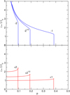 |
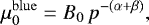
Fig. 4 Intensity profiles t(p) for pairs of positive and negative velocities, vz = ±1, ±21∕2, ±2. |
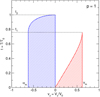 |
Fig. 5 Line profile showing the emission at a projected distance p as a function of LOS velocity. The blue wing emission encompasses LOS velocities from − vm to 0, and its peak value (at vz = 0) is t2 = p−1∕2. The red wing emission encompasses LOS velocities from 0 to vm = 0.620 p−1∕2, and its peak value (at vz = vm) is t1 = 0.760 p−1∕2. |
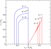 |
Fig. 6 Line profiles for values of p = 1, 21∕2, 2. |
4 First-order moment for an infinite infall radius
4.1 Dependence on the projected distance
We are interested in calculating the first-order normalized moment of the line profile as a function of the projected distance,
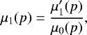 (13)
(13)
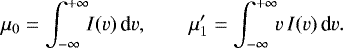
where μ0 and μ1 are the zeroth-order and unnormalized first-order moments,
 (14)
(14)
The moment μ0 has units of intensity times velocity, while μ1 has units of velocity.
From Eq. (8) we can obtain vz as an explicit function of t,
 (15)
(15)
where the blue-wing profile is obtained for 3−1∕4 p−1∕2 < t < p−1∕2, and the red-wing profile for 0 < t < 3−1∕4 p−1∕2. Since we know theinverse function vz(t), we can evaluate the integrals by integration by parts,
 (16)
(16)
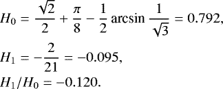
The details of the calculation of these integrals are given in Appendix A. As described inthe appendix, the final results obtained can be summarized as follows. The moments μ0,  , and μ1 are power laws of the projected distance p, and given by
![\begin{eqnarray*}\mu_0(p) &=& H_0\,p^{-1}, \nonumber\\ \mu'_1(p) &=& H_1\,p^{-3/2},\\ \mu_1(p) &=& [H_1/H_0]\,p^{-1/2}, \nonumber \end{eqnarray*}](/articles/aa/full_html/2019/06/aa34998-18/aa34998-18-eq33.png) (17)
(17)
A plot of the zeroth- and first-order moments can be seen in Fig. 7.
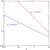 |
Fig. 7 Log–log plot of the moments μ0 and − μ1, as a functionof projected distance p. |
4.2 Effect of a finite spectral resolution
Let us assume that we are observing the lines with an spectrometer with a finite spectral resolution. The response of the spectrometer can be represented by the convolution of the “real” line profile with the instrumental response, which has a width equal to the spectral resolution. In general, we can assume that instrumental response is symmetric with respect to velocity. As shown in Appendix C, in this case the first-order moment of the line is not modified by the spectrometer.
4.3 Effect of a finite angular resolution
Let us assume that we are observing with a telescope with a circularly symmetric Gaussian beam with half-power beamwidth (HPBW) θb. In the following we will use the beamwidth in units of R0, that is, b ≡ D θb∕R0, where D is the distanceto the source.
The observed intensity as a function of projected distance will be the 2D convolution of t(p), given by Eq. (4), with the beam. Since the moments μ0 and  (but not μ1) depend linearly on the line profile t(p) (Eq. (14)), the convolution (a linear operator) can be performed onto μ0 and
  , and after that, obtain the normalized first-order moment
 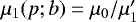 .
.
The 2D convolution of the power-law functions μ0 and  with a Gaussian beam has to be done numerically. However, it has to be done only once, because the result can be scaled for any value of b. For instance, if the numerical calculation has been done for b = 1 and μ1(p;1) is obtained, then for any value of b we have
 (19)
(19)
The function − μ1(p;1) is shown as a blue solid line in the log–log plot of Fig. 8.
However, since both μ0 and  are power laws of p, as shown in Appendix D, the value at the origin, p = 0, and the asymptotic expression for large projected distances, p ≫ b, can be obtained analytically. By application of Eqs. (D.8) and (D.10) to μ0 we obtain (see Fig. 8)
 (20)
(20)
with a characteristic size (the intersection of the two asymptotes) p0 = 0.339 b. For  we obtain
 (21)
(21)
with a characteristic size p1 = 0.254 b. Finally, for the first-order moment,  , we derive
 (22)
(22)
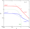 |
Fig. 8 Log–log plots of the moments μ0 and − μ1 (solid lines) for a Gaussian beam with HPBW b = 1 (dotted line), as a function of the projected distance p, and their asymptotic values (dashed lines) for p ≪ b and p ≫ b. |
5 First-order moment for a finite infall radius
Up to now we have assumed that the infall velocity pattern in r−1∕2 extends up to an infinite radius. A more realistic approach is to assume a finite radius. For instance, in the inside-out collapse model (Shu 1977), the collapse propagates outwards from the center at the speed of sound. The radius of the expansion wave is usually called the infall radius Ri, and let us call ri the infall radius in units of R0, that is, ri ≡ Ri∕R0. The envelope with a radius greater than the infall radius is approximately static, while the material inside the infall radius is in free fall. Thus, let us assume that the infall occurs only for radii r < ri. The static material will only contribute to the ambient-gas line-emission, centered on vz = 0, and will not be taken into account.
5.1 Line profile (finite infall radius)
The effect of having a finite infall radius is that the equal-LOS-velocity surfaces are truncated at a radius r = ri. Thus, for the red-wing emission, a part of the equal-LOS-velocity surface near the center of the core will no longer be hidden from the observer by the part facing the observer. A critical value of p is that for which the sphere of radius ri intersects the equal-LOS-velocity surfaces at the points (p = pm, z = zm), that is,  , or
, or  . As illustrated in Fig. 9, for a given projected distance
  , the blue-wing emission, like the infinite infall radius case, comes from material along the line of sight at radii
  . However, the red-wing emission, unlike the infinite infall radius case, comes from two regions: material along the line of sight at radii
 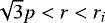 , in the part of the equal-LOS-velocity surface facing the observer, and material closer to the center, located at − zb < z < 0, which is no longer hidden by the part of the equal-LOS-velocity surface facing the observer because this part of the equal-LOS-velocity surface would be outside the infalling sphere of radius ri. The material in the part of the equal-LOS-velocity surface facing the observer has LOS velocities va < vz < vm, where va is the velocity of the material where the line of sight intersects the sphere of radius ri. The material closer to the center has LOS velocities 0 < vr < va (see Fig. 10).
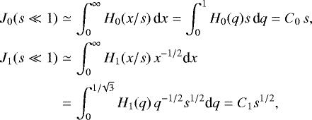
Let us use the reduced coordinate q ≡ p∕ri. The corresponding critical value of q is  (see Fig. 9). For values
  , only the red-wing emission is affected. For
  the line becomes symmetric because none of the red wing emission at any LOS velocity is hidden by the part of the equal-LOS-velocity surface facing the observer, and the moment μ1 becomes zero (see Figs. 9 and 10). For q ≥ 1 all the wing emission disappears (μ0 = μ1 = 0).
5.2 First-order moment (finite infall radius)
The details of the derivation of an analytical expression for the moments, for a finite infall radius are given in Appendix B. The moments μ0,  , and μ1 obtained are no longer power laws of the projected distance p, although the dependence on ri can be separated from the explicit dependence on p using the parameter q = p∕ri. In this way, the resulting expressions are similar to those obtained for the case of an infinite infall radius,
![\begin{eqnarray*}\hspace*{-7pt}&&\left.\begin{array}{l} \mu_0(p) = H_0(q)\,p^{-1} \\ \mu'_1(p) = H_1(q)\,p^{-3/2} \\ \mu_1(p) = [H_1(q)/H_0(q)]\,p^{-1/2} \end{array}\right\} \quad (0\leq q<1/\sqrt{3}), \nonumber\\ \hspace*{-7pt}&&\left.\begin{array}{l} \mu_0(p) = 2B_0\,p^{-1} \\ \mu'_1(p) = \mu_1(p)=0 \end{array}\right\} \quad (1/\sqrt{3}\leq q<1), \\ \hspace*{-7pt}&&\begin{array}{l} \mu_0(p) = \mu'_1(p) = \mu_1(p) =0 \end{array} \quad (q\ge1), \nonumber \end{eqnarray*}](/articles/aa/full_html/2019/06/aa34998-18/aa34998-18-eq55.png) (23)
(23)
with H0 and H1 given by (see Fig. B.2)
![\begin{eqnarray*} H_0(q) &=& 2B_0+[q(1-q^2)]^{1/2}({q'}^{1/2}-q^{1/2})-G_0(q)+G_0(q'),\nonumber \\ H_1(q) &=& \frac{q}{2}(1-q^2)({q'}^{1/2}-q^{1/2})-G_1(q)+G_1(q'), \end{eqnarray*}](/articles/aa/full_html/2019/06/aa34998-18/aa34998-18-eq56.png) (24)
(24)
where q′ is an auxiliary parameter depending on q only (see Fig. B.1),
![\begin{equation*} q'= \frac{1-q^2}{\left[1-\dfrac{q^2}{2}+\dfrac{q}{2}(4-3q^2)^{1/2}\right]^{1/2}}, \end{equation*}](/articles/aa/full_html/2019/06/aa34998-18/aa34998-18-eq57.png) (25)
(25)
An example of the moments obtained can be seen in Fig. 11.
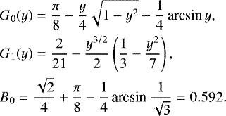
The limiting values of the moments for ri →∞, corresponding to q = 0, q′ = 1, coincide with the results derived for an infinite infall radius (Eqs. (17) and (18)),
 (27)
(27)
while the limiting values for  , corresponding to
 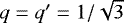 , are
, are
 (28)
(28)
 |
Fig. 9 For a given projected distance |

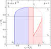 |
Fig. 10 Line profile for |


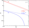 |
Fig. 11 Log–log plot of μ0 and − μ1 as a functionof the projected distance p, for an infall radius ri = 1 (solid lines) and for an infinite infall radius (dashed lines). |
5.3 Finite angular resolution (finite infall radius)
In this case, μ0 and  are no longer power laws of p, but have a characteristic scale size given by ri. Thus, unlike the infinite infall radius case, the beam convolution has to be performed for every value of ri, and the result will depend on both ri and b. For ri very large, the results for an infinite infall radius of the last section are reproduced.
6 Practical units
In the previous analysis all lengths, z, p, ri, b, are measured in units of the reference radius R0; velocities in units of V 0, the infall velocity at the reference radius R0; and temperatures in units of T0, the temperature at the reference radius R0. The projected distance p in practical units, that is, θ in arcsec, can be obtained from p in units of R0 through2
![\begin{equation*}\left[\frac{\theta}{\mathrm{arcsec}}\right]= p \left[\frac{R_0}{\mathrm{kau}}\right] \left[\frac{D}{\mathrm{kpc}}\right]^{-1}, \end{equation*}](/articles/aa/full_html/2019/06/aa34998-18/aa34998-18-eq64.png) (29)
(29)
where D is the distance to the source. The value of R0 is arbitrary, but the values of R0 and V 0 are related to the central mass of the protostar onto which the accretion is taking place, M*,
 (30)
(30)
![\begin{equation*}\left[\frac{V_0}{\mathrm{km~s}^{-1}}\right]=1.331 \left[\frac{M_{\ast}}{M_{\odot}}\right]^{1/2} \left[\frac{R_0}{\mathrm{kau}}\right]^{-1/2}. \end{equation*}](/articles/aa/full_html/2019/06/aa34998-18/aa34998-18-eq66.png)
6.1 Infinite infall radius
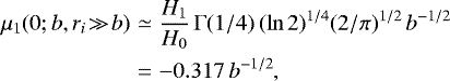
The first-order moment at the origin (Eq. (22)) in practical units becomes,
![\begin{equation*} \left[\frac{\mu_1(0;\theta_b)}{\mathrm{km~s}^{-1}}\right] = -0.317 \left[\frac{V_0}{\mathrm{km~s}^{-1}}\right] \left[\frac{R_0}{\mathrm{kau}}\right]^{1/2} \left[\frac{D}{\mathrm{kpc}}\right]^{-1/2} \left[\frac{\theta_b}{\mathrm{arcsec}}\right]^{-1/2}, \end{equation*}](/articles/aa/full_html/2019/06/aa34998-18/aa34998-18-eq67.png) (32)
(32)
![\begin{eqnarray*} \left[\frac{\mu_1(\theta;\theta_b)}{\mathrm{km~s}^{-1}}\right] \simeq -0.120 \left[\frac{V_0}{\mathrm{km~s}^{-1}}\right] \left[\frac{R_0}{\mathrm{kau}}\right]^{1/2} \left[\frac{D}{\mathrm{kpc}}\right]^{-1/2} \left[\frac{\theta}{\mathrm{arcsec}}\right]^{-1/2}.\hspace*{-10pt}\nonumber\\ \!\!\!\!\!\!\!\!\!\!\! \hfill \end{eqnarray*}](/articles/aa/full_html/2019/06/aa34998-18/aa34998-18-eq68.png)
Taking into account Eq. (30), we have for θ = 0
![\begin{equation*}\left[\frac{\mu_1(0;\theta_b)}{\mathrm{km~s}^{-1}}\right] = -0.423 \left[\frac{M_{\ast}}{M_{\odot}}\right]^{1/2} \left[\frac{D}{\mathrm{kpc}}\right]^{-1/2} \left[\frac{\theta_b}{\mathrm{arcsec}}\right]^{-1/2}, \end{equation*}](/articles/aa/full_html/2019/06/aa34998-18/aa34998-18-eq69.png) (34)
(34)
![\begin{equation*} \left[\frac{\mu_1(\theta;\theta_b)}{\mathrm{km~s}^{-1}}\right] \simeq -0.160 \left[\frac{M_{\ast}}{M_{\odot}}\right]^{1/2} \left[\frac{D}{\mathrm{kpc}}\right]^{-1/2} \left[\frac{\theta}{\mathrm{arcsec}}\right]^{-1/2}. \end{equation*}](/articles/aa/full_html/2019/06/aa34998-18/aa34998-18-eq70.png)
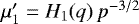
Examples of μ1(θ;θb) for some values of θb and M* are shown in Figs. 13 and 14. A value of the central mass can be derived directly from the value of the first-order moment at the origin,
![\begin{equation*}\left[\frac{M_{\ast}}{M_{\odot}}\right]= 5.6 \left[\frac{-\mu_1(0;\theta_b)}{\mathrm{km~s}^{-1}}\right]^2 \left[\frac{D}{\mathrm{kpc}}\right] \left[\frac{\theta_b}{\mathrm{arcsec}}\right]. \end{equation*}](/articles/aa/full_html/2019/06/aa34998-18/aa34998-18-eq71.png) (36)
(36)
It may seem surprising that the value of the first-order moment at the origin (Eq. (34)) does not depend on the temperature T0. This is because μ1 is the normalized moment  , and the dependence on T0 of both
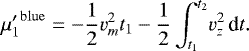
  and μ0 cancels. However, μ1 does depend on the temperature gradient, that is, on the power-law index of temperature law (β in Eq. (A.36)). For instance, for β = 0 (no temperature gradient), μ1 is zero.
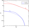 |
Fig. 12 Log–log plot of μ0 and − μ1 as a functionof the projected distance, for an infall radius ri = 1 and beamwidth b = 0.1 in reduced units (solid lines) and b = 0 (dashed lines). |
6.2 Finite infall radius
In this case the 2D convolution has to be computed for any value of the infall radius. A possible strategy for computing the first-order moment is the following.
- 1.
Choose avalue for R0, for instance R0 = 1 kau, so that the infall radius in reduced coordinates is ri = [Ri∕kau].
- 2.
For a given value of ri, and a range of values of p, construct the functions μ0 = H0(q) p−1 and
 (Eq. (23)) in reduced coordinates (p
and ri
in units of R0).
(Eq. (23)) in reduced coordinates (p
and ri
in units of R0). - 3.
Transform the p coordinate to practical units,
![$[\theta/\mathrm{arcsec}]=p\,[D/\mathrm{kpc}]^{-1}$](/articles/aa/full_html/2019/06/aa34998-18/aa34998-18-eq75.png) (Eq. (29)). Compute the beam 2D-convolution (Eq. (D.2)) of μ0
and
(Eq. (29)). Compute the beam 2D-convolution (Eq. (D.2)) of μ0
and  , and obtain
  . See in Fig. 12 an example of the resulting μ0
and μ1
after beam convolution.
. See in Fig. 12 an example of the resulting μ0
and μ1
after beam convolution. - 4.
The resulting first-order moment is in units of V 0. To have it in km s−1, scale μ1 by a factor
![$1.331\,[M_{\ast}/M_{\odot}]^{1/2}$](/articles/aa/full_html/2019/06/aa34998-18/aa34998-18-eq78.png) , where M*
is the central mass (Eq. (31)).
, where M*
is the central mass (Eq. (31)).
Examples of μ1(θ;θb, Ri) for some values of θb, Ri, and M* are shown in Figs. 15 and 16.
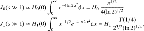
Let us see now what can be derived from the value of the first-order moment at the origin. The value of μ1 for θ = 0 (Eq. (B.38)) in practical units becomes
![\begin{eqnarray*} \left[\frac{\mu_1(0;\theta_b,R_i)}{\mathrm{km~s}^{-1}}\right] &=& \frac{J_1(s)}{J_0(s)} \left[\frac{V_0}{\mathrm{km~s}^{-1}}\right] \left[\frac{R_0}{\mathrm{kau}}\right]^{1/2} \left[\frac{D}{\mathrm{kpc}}\right]^{-1/2} \nonumber\\ && \times \, \left[\frac{\theta_b}{\mathrm{arcsec}}\right]^{-1/2}, \end{eqnarray*}](/articles/aa/full_html/2019/06/aa34998-18/aa34998-18-eq79.png) (37)
(37)
where s = Ri∕(Dθb), and J0 and J1 are given by Eq. (B.37). Taking into account Eq. (30), we have
![\begin{equation*} \left[\frac{\mu_1(0;\theta_b,R_i)}{\mathrm{km~s}^{-1}}\right] = J(s) \left[\frac{M_{\ast}}{M_{\odot}}\right]^{1/2} \left[\frac{D}{\mathrm{kpc}}\right]^{-1/2} \left[\frac{\theta_b}{\mathrm{arcsec}}\right]^{-1/2}, \end{equation*}](/articles/aa/full_html/2019/06/aa34998-18/aa34998-18-eq80.png) (38)
(38)
where J(s) = 1.331 J1(s)∕J0(s). The function J(s), calculated numerically, is shown in Fig. 17. The asymptotic expression for large infall radii, Ri ≫ Dθb,
![\begin{equation*} \left[\frac{\mu_1(0;\theta_b,R_i\!\gg\!D\theta_b}{\mathrm{km~s}^{-1}}\right] \simeq -0.423 \left[\frac{M_{\ast}}{M_{\odot}}\right]^{1/2} \left[\frac{D}{\mathrm{kpc}}\right]^{-1/2} \left[\frac{\theta_b}{\mathrm{arcsec}}\right]^{-1/2}, \end{equation*}](/articles/aa/full_html/2019/06/aa34998-18/aa34998-18-eq81.png) (39)
(39)
coincides, asexpected, with the expression derived for an infinite infall radius, Eq. (34). In the case of a poor angular resolution compared with the infall radius (θb ≫ Ri∕D), we obtain
![\begin{equation*} \left[\frac{\mu_1(0;\theta_b\!\gg\!R_i/D,R_i)}{\mathrm{km~s}^{-1}}\right] \simeq -0.080 \left[\frac{M_{\ast}}{M_{\odot}}\right]^{1/2} \left[\frac{R_i}{\mathrm{kau}}\right]^{-1/2}. \end{equation*}](/articles/aa/full_html/2019/06/aa34998-18/aa34998-18-eq82.png) (40)
(40)
The value at the origin of the first-order moment in the case of a finite infall radius, μ1 (0;θb, Ri), in contrast with the infinite infall radius case, does not provide a unique value of the central mass, unless the infall radius is known. There is a degeneracy between the infall radius and the central mass: different pairs of values of the infall radius and central mass produce the same value of the first-order moment at the origin. In order to disentangle this degeneracy, it is necessary to fit not only the value at the origin, but also the variation of the observed first-order moment as a function of the projected distance.
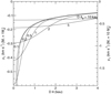 |
Fig. 13 First-order moment μ1 for an infinite infall radius, as a function of the projected distance, D θ (in kau), for beamwidths D θb = 0.1, 0.2, 0.5, 1, 2, 5, and 10 kau, where D is the distance to the source. The vertical axis scales as |

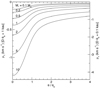 |
Fig. 14 First-order moment μ1 for an infinite infall radius, as a function of the projected distance in units of the beamwidth, θ∕θb (adimensional), for central masses M* = 0.1, 0.2, 0.5, 1, 2, 5, and 10 M⊙. The vertical axis scales as |

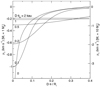 |
Fig. 15 First-order moment μ1, as a functionof projected distance in units of the infall radius, D θ∕Ri (adimensional), for beamwidths D θb = 0, 0.1, 0.2, 0.5, 1, and 2 kau, where D is the distance to the source. The vertical axis scales as |

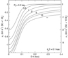 |
Fig. 16 Same as Fig. 15, for D θb = 0.1 kau, and Ri = 0.2, 0.5, 1, 2, 5, 10, and ∞ kau. The horizontal axis is the projected distance, D θ (in kau). Note that the line for Ri = 1 kau in this figure coincides with the line for D θb = 0.1 kau in Fig. 15. |
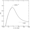 |
Fig. 17 Function J(s) in the expression of μ1(0;θb, Ri), showing its asymptotic values for s ≪ 1 and s ≫ 1. |
7 Application of the central-blue-spot infall hallmark to real data
7.1 G31.41+0.31 HMC
G31.41+0.31 HMC (hereafter G31) is a hot molecular core whose distance was estimated to be 7.9 kpc, but recent determinations (Reid et al., in prep.) give a value of 3.7 kpc for its distance. Infall motions in G31 have been reported by Girart et al. (2009) from inverse P-Cygni profiles, and by Mayen-Gijon et al. (2014) from VLA observations of the ammonia inversion transitions (2, 2), (3, 3), (4, 4), (5, 5), and (6, 6) showing a central blue-spot in the first-order moment maps.
Here we are analyzing the first-order moment maps shown in Fig. 2 of Mayen-Gijon et al. (2014) (see Fig. 18). The half-power beamwidth of the observations were 0.′′ 33 for the (2, 2), (3, 3), and (6, 6) maps, 0.′′ 16 for the (4, 4) map, and 0.′′ 37 for the (5, 5) map. The value of the first-order moment as a function of the angular distance was obtained for the five maps by averaging the first-order moment in concentric rings of width 0.′′1 centered onthe average position of the peak of the blue spot, α(J2000) = 18h47m34.s32, δ(J2000) = −01°12′46.′′1. In Fig. 19, we present the first-order moment profiles obtained. We considered that the velocity far from the center was 97.4 km s−1, the value used by Mayen-Gijon et al. (2014), which is consistent with the values of the systemic velocity quoted for G31, ranging from 96.26 km s−1 (Beltrán et al. 2005) to 98.8 km s−1 (Cesaroni et al. 1994).The first-order moment of the different transitions show very similar profiles, with a value of approximately − 3 km s−1 for small angular distances, except for the (2, 2) transition, which shows a shallower dip in velocity. This could be due to a lower opacity of the (2, 2) line, and partial blending of the central line with the inner satellite lines, and we will no longer consider this transition. By application of Eq. (36) we see that a value of ~ − 3 km s−1 for the first-order moment means roughly a central mass of the order of 50 M⊙.
In order to obtain a more accurate value of the central mass, the hallmark model was calculated for the beam size of each transition, and fitted to the observed data for different values of the infall radius and the central mass. For an infinite infall radius the best fit was found for a central mass of 44 M⊙, with a residual χ2 statistic for ν = 39 degrees of freedom (the total number of rings of all transitions used in the fit, minus 1), χ2 = 36.6, which gives a reduced 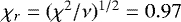 . For finite values of the infall radius we obtained higher values of the central mass. For Ri = 20 kau (corresponding to an angular radius of 5.′′ 4 at 3.7 kpc), we obtained a better fit, with a central mass M* = 69M⊙ (χ2 = 21.2, χr = 0.74), while for Ri = 5 kau (1.′′ 4), a lower limit for the infall radius to be consistent with the size of the NH3 maps, the best fit was for a central mass M* = 122 M⊙ (χ2 = 10.7, χr = 0.52) (see Fig. 20). In conclusion, the central mass obtained is always greater than ~ 44 M⊙, and the best fit is obtained for values of the infall radius between 5 and 20 kau, with central masses between ~ 70 and ~ 120 M⊙.
Osorio et al. (2009) model and the central core of G31 obtain, assuming a distance of 7.9 kpc, a central star with a mass of ~ 25M⊙, a mass accretion rate of 3 × 10⁻³ M⊙ yr−1, and a total luminosity of 2 × 10⁵ L⊙. The luminosity, scaled to the distance of 3.7 kpc adopted here, is 4.4 × 10⁴ L⊙. A single star with a mass equal to the central mass derived here would have a luminosity two orders of magnitude higher. This apparent lack of luminosity can be explained considering, as usually found in high-mass star forming regions, that there is not a single high-mass star at the center of G31, but a cluster of less massive stars. In the case of G31, recent high-angular resolution ALMA continuum observations (Beltrán et al., in prep.) reveal the presence of at least four cores at the center of G31.
If we assume that the stars of the cluster at the center of G31 have masses that follow the Salpeter initial mass function (Salpeter 1955) there would be a few high-mass young stellar objects, probably associated with the four cores detected, which could account for most of the total luminosity observed. A higher number of low-mass young stellar objects yet undetected, with little contribution to the overall luminosity, could total a mass of 70–120 M⊙ for the cluster.
 |
Fig. 18 Maps of G31 first-order (color scale) and zeroth-order moment (contours) for the ammonia inversion transitions (2, 2) to (6, 6) (Mayen-Gijon et al. 2014). The color scale, the same for all panels, ranges from 94 to 101 km s−1. The contours are in steps of 10% of the peak value for all the maps, except for the (4, 4) transition, for which the steps are 20%. The beam is shown in the lower right corner of each panel. |
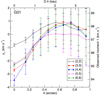 |
Fig. 19 G31 first-order moment for the ammonia inversion transitions (2, 2) (black line and open circles), (3, 3) (red line andfilled circles), (4, 4) (blue line and filled squares), (5, 5) (magenta line and open squares), and (6, 6) (green line and filled diamonds) (Mayen-Gijon et al. 2014), as a function of angular distance, measured for rings of width 0.′′ 1 and average radius θ. The error bars are the rms of the velocity inside each ring. The right-hand vertical axis shows the velocities obtained from the first-order moment maps, while the left-hand vertical axis shows the velocity with respect to the systemic velocity of G31, taken as V sys = 97.4 km s−1. |
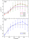 |
Fig. 20 Model (black dashed line) fitted to the G31 first-order moment, calculated for a central mass of 122 M⊙, an infall radius of 5 kau, and a half-power beamwidth of ~0.′′33 for the (3, 3), (5, 5), and (6, 6) transitions (top), and 0.′′16 for the (4, 4) transition (bottom). |
7.2 B335
B335 is an isolated Class 0 protostar with a bolometric luminosity of ~ 1 L⊙, at a distance of 105 pc (Olofsson & Olofsson 2009). Several authors claim the detection of infall (Kurono et al. 2013; Evans et al. 2015). Here we are analyzing two observations, one of H13 CO+ (J = 1–0) at 87 GHz, with a moderate angular resolution, combining data from the 45 m Nobeyama telescope and the Nobeyama Millimeter Array (Kurono et al. 2013), and the other of 13CO (J = 2–1) at 220 GHz, with very high angular resolution, carried out with the Atacama Large Millimeter/Submillimeter Array (ALMA; Yen et al. 2015).
Regarding the Nobeyama data, the beam obtained for the combined data from both instruments was ~ 5.′′0, and the spectral resolution was 0.108 km s−1. The channel maps of the H13 CO+ emission were retrieved from Fig. 5 of Kurono et al. (2013), and the data cube obtained was resampled with a cell size of 1″. The zeroth and first-order moments obtained are shown in Fig. 21. The value of the first-order moment as a function of the angular distance was obtained by averaging the first-order moment in concentric rings of width 2″ centered onthe position of the continuum compact source, α(J2000) = 19h37m00.s89, δ(J2000) = +07°34′09.′′6 (Yen et al. 2015), the (0, 0) position in Figs. 21 and 22. The values obtained are shown in Fig. 23 (top panel). The error bars are the rms dispersion of velocities inside each ring, added quadratically to the uncertainty due to the finite spectral resolution, the same for all rings.
The ALMA data had an angular resolution of ~ 0.′′31, and the spectral resolution was 0.166 km s−1. The first-order moment for all the line, μ1, is shown in the middle panel of Fig. 22. As can be seen, the central blue spot is not centered on the position of the continuum compact source (plus sign), but is offset and extends to the southeast. The angular resolution of the data corresponds to a linear resolution of 33 au at a distance of 105 pc. At this small scale, the kinematics can be dominated by the rotation of the protostellar disk, and infall can be no longer spherically symmetric, as assumed by the hallmark model. In order to check the validity of the model, we also computed the first order moment separately for the redshifted channels, with velocity higher than the systemic velocity,  , and for the blueshifted channels (with velocity lower than V sys),
  . The hallmark model predicts that
  shows a central redspot and
  a central blue spot, higher in absolute value than the first-order moment of the full line. As can be seen in the top and bottom panels of Fig. 22, this is what is observed for
  and
and  , with quite well centered red and blue spots. The values of μ1,
  , and
, and  as a function of the angular distance were calculated for concentric rings of 0.′′ 1 width, centered on the position of the continuum compact source. The error bars were calculated in the same way as for the Nobeyama data. The moments as a function of the angular distance θ, are shown in Fig. 23 (bottom panel). As can be seen, the three moments follow the same kind of dependence on the projected distance, and we will see that they can be fitted by power laws of index − 1∕2, convolved with the beam, as predicted by the hallmark model. Thus, the gas kinematics for the range of projected distances sampled by ALMA, from 0.′′ 1 to 0.′′ 8 (10–84 au), appears to be dominated by infall.
The hallmark model was calculated and fitted simultaneously to the Nobeyama first-order moment μ1, and to the ALMA  and
and  (but not to μ1). Since the Nobeyama data are very sensitive to the value adopted for the systemic velocity, we fitted both the value of the systemic velocity and the central mass. We tested the infall radius reported by Kurono et al. (2013), 2900 au (corrected from their assumed distance of 150 pc), but a better fit was obtained with a larger infall radius. The best fit was obtained for an infinite infall radius, for a systemic velocity V sys = 8.29 km s−1, and central mass M* = 0.09M⊙ (dashed lines in the top and bottom panels of Fig. 23). The goodness of the fit is given by a χ2 statistic for ν = 27 degrees of freedom, χ2 = 29.9, corresponding to a reduced
  , an indication that the model fits well the data within the uncertainties. As an additional check, we computed the predicted value of the first-order moment for the ALMA data of the full line, μ1, (dotted line in the bottom panel of Fig. 23), which is a linear combination of
  and
and  , that is,
  . As can be seen in the figure, the values predicted for μ1 match well those observed.
We can conclude that the kinematics of the gas in B335, for the linear scales sampled by ALMA and Nobeyama, from ~ 10 to ~ 2500 au, in other words, more than two orders of magnitude, can be explained by a simple model of infall onto a central protostar of ~ 0.1 M⊙. This can be considered as an outstanding result of the central-blue-spot infall hallmark model.
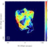 |
Fig. 21 B335 zeroth-order (contours) and first-order moment (color scale) of the H13 CO+ (J = 1–0) line, obtained from the channel maps of Kurono et al. (2013). Contours are in steps of 511 mJy beam−1 km s−1. The color scale at the right border is in m s−1. The (0, 0) position corresponds to α(J2000) = 19h37m00.s89, δ(J2000) = +07°34′09.′′6. The synthesized beam is shown in the lower left corner. |
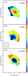 |
Fig. 22 B335 first-order moment of the 13CO (J = 2–1) line observed with ALMA. Top: moment of the red channels, with velocities higher than the systemic velocity, V sys (color scale: 8.9–10.1 km s−1). Middle: moment of all the channels (color scale: 7.4–9.2 km s−1). Bottom: moment of the blue channels, with velocities lower than V sys (color scale: 6.8–8.0 km s−1). The (0, 0) position, marked with a plus sign, is the same as in Fig. 21. The synthesized beam is shown in the lower left corner of the middle panel. |
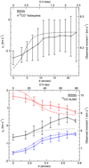 |
Fig. 23 Same as Fig. 19 for B335. Top: H13CO+ (J = 1–0) line observed at Nobeyama (2″ ring width). Bottom: 13CO (J = 2–1) line observed with ALMA (0.′′1 ring width; |


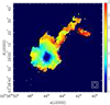 |
Fig. 24 NH3 (1, 1) line central velocity of the Guitar Core in L1287. The central blue spot is blueshifted ~ 0.5 km s−1 with respect to the ambient gas. The embedded sources in the center are indicated by dots (mm, Juárez et al. 2019), and crosses (cm, Anglada et al. 1994). The synthesized beam is shown in the lower-right corner of the map. |
7.3 LDN 1287
LDN 1287 (hereafter L1287) is a molecular cloud located at a distance of 929 pc, associated with an energeticbipolar CO outflow (Yang et al. 1991). The source was mapped with a single dish in NH3 (Estalella et al. 1993; Sepúlveda et al. 2011). A cluster of mm sources has been detected at the center of L1287 (Juárez et al. 2019), one of the mm sources being associated with VLA 3 (Anglada et al. 1994), a jet-like cm-continuum source that appears to be driving the outflow.
Here we are analyzing VLA observations of the NH3 (1, 1) and (2, 2) transitions, which show a complicated structure with a complex kinematics (Sepúlveda et al. in prep.). The NH3 lines were analyzed by means of the Hyperfine Structure Tool (HfS) (Estalella 2017). After careful inspection of the spectra, three different velocity components were identified, with non-overlapping velocity ranges (Guitar Core, Blue Filament, and Red Filament). The Guitar Core does not show any sign of interaction with the embedded young stellar objects (no increase in linewidth, nor in rotational temperature at the projected position of the embedded sources). Our results suggest that the Guitar core is a very young protostellar core. Given the poor velocity resolution of the observations, the only way to separate the emission of the Guitar Core from that of the filaments was to fit Gaussian components to the observed spectra. Thus, the asymmetry of the line was inferred from the shift of the central velocity of the line fitted. Nevertheless, a compact spot of ~ 10″ in diameter of blueshifted velocities appears at the center of the Guitar Core (see Fig. 24).
The central velocity of the Guitar Core, obtained from the HfS fits, was averaged in concentric rings 1″ wide, centered on the emission peak, up to a radius of 20″. The velocity profile obtained is shown in Fig. 25. The error bars are the rms dispersion of the velocities averaged in each ring, added quadratically to the error of the average value of central velocity obtained from HfS. The average velocity at large distances from the peak (the systemic velocity of the Guitar Core), − 18.54 km s−1, has been subtracted from the values of the central velocity. The best fit to the (1, 1) and (2, 2) data, for a beamwidth of 3.′′ 48, was obtained for a central massof 4.8 M⊙ and a infinite infall radius (dashed line in Fig. 25). The goodness of the fit is indicated by the value of the χ2 statistic for ν = 39 degrees of freedom (the total number of rings used in the fit, minus 1), χ2 = 42.7, which gives a reduced  .
.
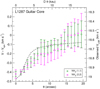 |
Fig. 25 Same as Fig. 19 for the Guitar Core in L1287, for the NH3 (1, 1) (blue circles)and (2, 2) lines (red circles). The rings used were 1″ wide, and a systemic velocity V sys = −18.55 km s−1 was adopted. The best fit was obtained for an infinite infall radius, and a central mass M* = 4.4 M⊙ (black dashed line). |
8 Conclusions
The central-blue-spot infall hallmark (Mayen-Gijon et al. 2014) was studied quantitatively, taking as a basis the work of Anglada et al. (1987, 1991). The assumptions were that the line emission was optically thick, the gravitational infall motions dominated the kinematics over turbulent and thermal motions, the infall velocity and temperature were power-laws of radius and increase inwards, with power-law indices of − 1∕2, and that the Sobolev approximation was valid. With these assumptions an analytical expression for the first-order moment as a function of the projected distance was derived, for the cases of infinite and finite infall radius. The effect of a finite angular resolution was also studied, but the convolution with the beam has to be calculated numerically. These results were applied to existing data of several star-forming regions (G31, B335, and L1287), obtaining good fits to the first-order moment maps, and deriving values of the central masses onto which the infall is taking place. The values obtained for the central masses are 70–120 M⊙ for G31, 0.1 M⊙ for B335, and 4.8 M⊙ for the Guitar Core of L1287.
In conclusion, the central-blue-spot infall hallmark appears to be a robust and reliable indicator of infall.
Acknowledgements
This work has been partially supported by the Spanish MINECO grants AYA2014-57369-C3 and AYA2017-84390-C2 (cofunded with FEDER funds), by MDM-2014-0369 of ICCUB (Unidad de Excelencia “María de Maeztu”), and through the “Center of Excellence Severo Ochoa” award for the Instituto de Astrofísica de Andalucía (SEV-2017-0709).
Appendix A Calculation of the moments for an infinite infall radius and arbitrary power-law indices
A.1 Intensity profile (infinite infall radius)
Let us assume that the infall velocity and temperature in an infalling molecular gas core are given by power laws with arbitrary power-law indices, − α and − β,
 (A.1)
(A.1)
The development made in Sect. 2 for α = β = 1∕2 can be generalized for any positive values of the power-law indices, α, β > 0. The projected distance and temperature (Eq. (4)) are now
 (A.2)
(A.2)
The expressions for z*, zm, pm (Eq. (5)) become
 (A.3)
(A.3)
and t(pm) (Eq. (6)) is now
 (A.4)
(A.4)
A.2 Line profile (infinite infall radius)
The equations derived in Sect. 3 can be generalized as follows. The temperature and LOS velocity (Eq. (8)) become
 (A.5)
(A.5)
The velocity vm and temperatures t1 and t2 (Eqs. (9), (10), (12)) are now given by
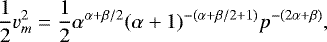
![\begin{eqnarray}&&\hspace*{-6pt} v_m = \alpha^{\alpha/2}(\alpha+1)^{-(\alpha+1)/2}\,p^{-\alpha},\nonumber\\ &&\hspace*{-6pt} t_1 = [\alpha/(\alpha+1)]^{\beta/2}\,p^{-\beta}, \\ &&\hspace*{-6pt} t_2 = p^{-\beta}. \nonumber \end{eqnarray}](/articles/aa/full_html/2019/06/aa34998-18/aa34998-18-eq104.png) (A.6)
(A.6)
A.3 Moments calculation (infinite infall radius)
From Eq. (A.5) we can obtain vz as an explicit function of t,
 (A.7)
(A.7)
where the blue-wing profile (vz < 0) is obtained for t1 < t < t2, and the red-wingprofile (vz > 0) for 0 < t < t1 (see Eq. (A.6)).
In order to calculate the first-order normalized moment μ1 (p) as a function of the projected distance,
 (A.8)
(A.8)
we need to evaluate the integrals
 (A.9)
(A.9)
A.4 Zeroth-order moment (infinite infall radius)
For the blue wing, the limits of integration are from (t = t1, vz = −vm) to (t = t2, vz = 0). The resulting integral for  is
is
 (A.10)
where vm, t1, and t2 have already been defined in Eq. (A.6). The first term is
 (A.11)
The integral of the second term has the same dependence on p. This can be seen with the change of variables x = pt1∕β, resulting in
![\begin{equation*} \int_{t_1}^{t_2}\! |v_z|\,\textrm{d}t= p^{-(\alpha+\beta)}\int_{\![\alpha/(\alpha+1)]^{1/2}}^1 \beta x^{\alpha+\beta-1}\sqrt{1-x^2}\,\textrm{d}x. \end{equation*}](/articles/aa/full_html/2019/06/aa34998-18/aa34998-18-eq111.png) (A.12)
(A.12)
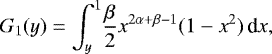
It is useful to define the function G0,
 (A.13)
which, in general, is not analytical, but is convergent for α + β > 0, and the function to integrate is continuum for x > 0. With this notation, the zeroth-order moment can be expressed as
 (A.14)
![\begin{equation*} B_0= \alpha^{(\alpha+\beta)/2}(\alpha+1)^{-(\alpha+\beta+1)/2} +G_0\left([\alpha/(\alpha+1)]^{1/2}\right). \end{equation*}](/articles/aa/full_html/2019/06/aa34998-18/aa34998-18-eq114.png)
Similarly, for the red wing the limits of integration are from (t = 0, vz = 0) to (t = t1, vz = vm). The resulting integral for  is
is
 (A.16)
Using the same notation used for the blue wing, we can obtain
 (A.17)
is analytical for α + β > 0, and its value is
![\begin{equation*} G_0(0)= \frac{\beta \sqrt{\pi}}{4} \frac{\Gamma\left[(\alpha+\beta)/2\right]}{\Gamma\left[(\alpha+\beta+3)/2\right]}, \end{equation*}](/articles/aa/full_html/2019/06/aa34998-18/aa34998-18-eq120.png) (A.20)
(A.20)
where Γ is the Gamma function.
Thus, the expression for the total zeroth-order moment is
 (A.21)
![\begin{eqnarray*} H_0 &=& 2B_0-G_0(0) = 2\alpha^{(\alpha+\beta)/2}(\alpha+1)^{-(\alpha+\beta+1)/2} \nonumber\\ && -\, {}\frac{\beta \sqrt{\pi}}{4} \frac{\Gamma\left[(\alpha+\beta)/2\right]}{\Gamma\left[(\alpha+\beta+3)/2\right]} +2G_0\left([\alpha/(\alpha+1)]^{1/2}\right). \end{eqnarray*}](/articles/aa/full_html/2019/06/aa34998-18/aa34998-18-eq122.png)
A.5 First-order moment (infinite infall radius)
For the blue wing, using the same limits of integration as for the zeroth-order moment, we have (see Fig. 5)
 (A.23)
and the integral can be evaluated using the same change of variables as for the zeroth-order moment, obtaining
![\begin{equation*} \frac{1}{2}\int_0^{t_2}\! v_z^2\,\textrm{d}t= G_1\left([\alpha/(\alpha+1)]^{1/2}\right) p^{-(2\alpha+\beta)}, \end{equation*}](/articles/aa/full_html/2019/06/aa34998-18/aa34998-18-eq125.png) (A.25)
(A.25)
where we defined the function G1 as
 (A.26)
which is analytical, and convergent for 2α + β > 0,
![\begin{equation*} G_1(y) = \frac{\beta}{(2\alpha+\beta)(2\alpha+\beta+2)} - \frac{\beta y^{2\alpha+\beta}}{2}\left[\frac{1}{2\alpha+\beta}-\frac{y^2}{2\alpha+\beta+2}\right]. \end{equation*}](/articles/aa/full_html/2019/06/aa34998-18/aa34998-18-eq127.png) (A.27)
(A.27)
Thus, the unnormalized first-order moment of the blue wing can be expressed as
 (A.28)
![\begin{equation*} B_1= -\frac{1}{2} \alpha^{\alpha+\beta/2} (\alpha+1)^{-(\alpha+\beta/2+1)} -G_1\left([\alpha/(\alpha+1)]^{1/2}\right). \end{equation*}](/articles/aa/full_html/2019/06/aa34998-18/aa34998-18-eq129.png)
Similarly, for the red wing we have
 (A.30)
that can be expressed as
 (A.31)
![\begin{equation*} R_1= \frac{1}{2} \alpha^{\alpha+\beta/2} (\alpha+1)^{-(\alpha+\beta/2+1)} +G_1\left([\alpha/(\alpha+1)]^{1/2}\right)-G_1(0). \end{equation*}](/articles/aa/full_html/2019/06/aa34998-18/aa34998-18-eq132.png)
Note that B1 and R1 cancel each other partially, so that
 (A.33)
Thus, the expression for the total unnormalized first-order moment is simply
 (A.34)
The final results, for an infinite infall radius, can be summarized as follows.
![\begin{eqnarray*}\mu_0 &=& H_0\,p^{-(\alpha+\beta)}, \nonumber\\ \mu'_1 &=& H_1\,p^{-(2\alpha+\beta)}, \nonumber\\ \mu_1 &=& [H_1/H_0]\,p^{-\alpha}, \\ H_0 &=& 2\alpha^{(\alpha+\beta)/2}(\alpha+1)^{-(\alpha+\beta+1)/2} -\frac{\beta \sqrt{\pi}}{4} \frac{\Gamma\left[(\alpha+\beta)/2\right]}{\Gamma\left[(\alpha+\beta+3)/2\right]} \nonumber\\ && +\, 2G_0\left([\alpha/(\alpha+1)]^{1/2}\right),\nonumber\\ H_1 &=& -\frac{\beta}{(2\alpha+\beta)(2\alpha+\beta+2)}, \nonumber \end{eqnarray*}](/articles/aa/full_html/2019/06/aa34998-18/aa34998-18-eq136.png) (A.36)
(A.36)
where Γ is the Gamma function, and
 (A.37)
which, in general, has to be evaluated numerically.
A.6 Particular case (infinite infall radius) for power-law indices 1/2
For the particular case of α = β = 1∕2, the former expressions are simpler. In particular, the integral G0 is analytical,
 (A.38)
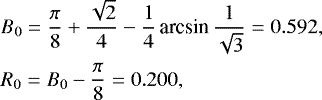
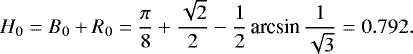
For the first-order moment we have
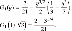 (A.42)
It can be useful to give the normalized first-order moment separately for the blue and red wings,
![\begin{eqnarray*} &&\hspace*{-6pt} \mu_1^{\mathrm{blue}} = [B_1/B_0]\,p^{-1/2} = -0.302\,p^{-1/2}, \nonumber\\ &&\hspace*{-6pt} \mu_1^{\mathrm{red}} = [R_1/R_0]\,p^{-1/2} = \phantom{-}0.418\,p^{-1/2}, \end{eqnarray*}](/articles/aa/full_html/2019/06/aa34998-18/aa34998-18-eq145.png) (A.45)
(A.45)
which have the same power-law dependence on the projected distance as μ1.
In conclusion, for the total zeroth and first-order moments we have
![\begin{eqnarray*} \mu_0 &=& H_0\,p^{-1} = 0.792\,p^{-1}, \nonumber\\ \mu'_1 &=& H_1\,p^{-3/2} = -0.095\,p^{-3/2}, \\ \mu_1 &=& [H_1/H_0]\,p^{-1/2} = -0.120\,p^{-1/2}. \nonumber \end{eqnarray*}](/articles/aa/full_html/2019/06/aa34998-18/aa34998-18-eq146.png) (A.46)
(A.46)
Appendix B Calculation of the moments for a finite infall radius and arbitrary power-law indices
The critical value of the reduced coordinate q = p∕ri, for an arbitrary value of the power-lax index α, is ![$q=[\alpha/(\alpha+1)]^{1/2}$](/articles/aa/full_html/2019/06/aa34998-18/aa34998-18-eq147.png) . For values
. For values ![$q<[\alpha/(\alpha+1)]^{1/2}$](/articles/aa/full_html/2019/06/aa34998-18/aa34998-18-eq148.png) , only the red-wing emission is affected; for
, only the red-wing emission is affected; for ![$q\ge[\alpha/(\alpha+1)]^{1/2}$](/articles/aa/full_html/2019/06/aa34998-18/aa34998-18-eq149.png) the line becomes symmetric (μ1 = 0); for q ≥ 1 all the wing emission disappears (μ0 = μ1 = 0).
the line becomes symmetric (μ1 = 0); for q ≥ 1 all the wing emission disappears (μ0 = μ1 = 0).
B.1 Line profile (finite infall radius)
In order to calculate the moments of the red wing emission we need the values of va, ta, and tb as a function of p and q (see Fig. 10). For this, we need the values of za and zb, the z coordinate of the two intersections of the equal-LOS-velocity surface with the line-of-sight.
The distance za is obtained readily from  , which gives
 (B.1)
(B.1)
and, from Eq. (A.6) we have
 (B.2)
(B.2)
 |
Fig. B.1 Plot of q′ as a functionof q (case α = β = 1∕2), for |

The distance zb requires more work. The equation of the equal-LOS-velocity surface of velocity va (Eq. (A.6)) can be written as
 (B.3)
(B.3)
For a given p and va, zb is a root of this equation that satisfies 0 < zb < za. It is useful to use the variable  , so that the equation to solve depends only on q and α, and becomes
 (B.4)
(B.4)
For rational values of α this equation is a polynomial in x. However, in general, the root has to be found numerically. An iterative algorithm that gives the correct root for ![$q<[\alpha/(\alpha+1)]^{1/2}$](/articles/aa/full_html/2019/06/aa34998-18/aa34998-18-eq156.png) is the following
is the following
 (B.5)
(B.5)
It is useful to introduce the parameter q′, which plays a role similar to that of q,
 (B.6)
(B.6)
so that the temperature tb, corresponding to zb, can be expressed as
 (B.7)
(B.7)
It can be easily shown that for ![$q<[\alpha/(\alpha+1)]^{1/2}$](/articles/aa/full_html/2019/06/aa34998-18/aa34998-18-eq160.png) , the parameter q′ is always bounded by q < q′ < 1, and that for
, the parameter q′ is always bounded by q < q′ < 1, and that for ![$q=[\alpha/(\alpha+1)]^{1/2}$](/articles/aa/full_html/2019/06/aa34998-18/aa34998-18-eq161.png) , q′ = q (see Fig. B.1).
, q′ = q (see Fig. B.1).
B.2 Zeroth-order moment (finite infall radius)
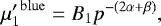
The zeroth-order moment of the blue wing,  , does not depend on q, and we havealready seen that it can be expressed as
 (B.8)
(B.8)
The zeroth-order moment of the red wing,  , can be calculated as
 (B.9)
(B.9)
Using the expressions obtained for va, ta, and tb,  can be expressed as
 (B.10)

where q′ is given by Eq. (B.6), and G0 by Eq. (A.13).
Finally, the total zeroth-order moment can be written as
![\begin{equation*} \mu_0 = [B_0+R_0(q)]\,p^{-(\alpha+\beta)}= H_0(q)\,p^{-(\alpha+\beta)}, \end{equation*}](/articles/aa/full_html/2019/06/aa34998-18/aa34998-18-eq169.png) (B.12)
(B.12)

B.3 First-order moment (finite infall radius)
The first-order moment for the blue wing does not depend on q, and we have already seen that
 (B.14)
The first-order moment of the red wing is the opposite of  , except for a deficit of red-wing emission (see Fig. 10), so that
 (B.15)
Taking into account the expressions of va, ta, and tb, the first-order moment of the red wing can be written as
 (B.16)
where q′ is given by Eq. (B.6), and G1 by Eq. (A.26). Thus, the total unnormalized first-order moment is
![\begin{equation*} \mu'_1 = [B_1+R_1(q)]\,p^{-(2\alpha+\beta)} = H_1(q)\,p^{-(2\alpha+\beta)}, \end{equation*}](/articles/aa/full_html/2019/06/aa34998-18/aa34998-18-eq176.png) (B.18)
(B.18)
The normalized first order moments for the blue and red wings separately are given by
![\begin{eqnarray*} &&\hspace*{-6pt} \mu_1^{\mathrm{blue}} = [B_1/B_0]\,p^{-\alpha}, \nonumber\\ &&\hspace*{-6pt} \mu_1^{\mathrm{red}} = [R_1(q)/R_0(q)]\,p^{-\alpha}, \end{eqnarray*}](/articles/aa/full_html/2019/06/aa34998-18/aa34998-18-eq178.png) (B.20)
(B.20)
where B0, B1, R0 (q), and R1 (q) have already been given. Finally, the expression obtained for the normalized first-order moment of the whole line,  , is
, is
 (B.21)
B.4 Final results (finite infall radius)
Assuming infall velocity and temperature that are power laws of the radius,
 (B.22)
we have, for a finite infall radius ri, with q = p∕ri,
![\begin{eqnarray*}&&\hspace{-7pt}\left.\begin{array}{l} \mu_0(p) = H_0(q)\,p^{-(\alpha+\beta)} \\ \mu'_1(p) = H_1(q)\,p^{-(2\alpha+\beta)} \\ \mu_1(p) = [H_1(q)/H_0(q)]\,p^{-\alpha} \end{array}\right\} \quad (0\leq q<[\alpha/(\alpha+1)]^{1/2}), \nonumber\\ &&\hspace{-7pt}\left.\begin{array}{l} \mu_0(p) = 2B_0\,p^{-(\alpha+\beta)} \\ \mu'_1(p) = \mu_1(p)=0 \end{array}\right\} \quad ([\alpha/(\alpha+1)]^{1/2}\leq q<1), \\ &&\hspace{-7pt}\begin{array}{l} \mu_0(p) = \mu'_1(p) = \mu_1(p) =0 \end{array} \quad (q\ge1), \nonumber \end{eqnarray*}](/articles/aa/full_html/2019/06/aa34998-18/aa34998-18-eq182.png) (B.23)
(B.23)
with H0(q) and H1(q) given by
 (B.24)
where q′ is an auxiliary parameter
 (B.25)
and x is the root, satisfying 0 < x < q−2, of the equation
 (B.26)
to be solved numerically (see Eq. (B.5)), and
![\begin{eqnarray*} &&\hspace*{-6pt} G_0(y) = \int_y^1\! \beta x^{\alpha+\beta-1}\sqrt{1-x^2}\,\textrm{d}x \quad\mbox{(to be done numerically),} \nonumber\\ &&\hspace*{-6pt} G_1(y) = \frac{\beta}{(2\alpha+\beta)(2\alpha+\beta+2)} \nonumber\\ &&\hspace*{20pt} \quad - \,\frac{\beta y^{2\alpha+\beta}}{2} \left[\frac{1}{2\alpha+\beta}-\frac{y^2}{2\alpha+\beta+2}\right], \\ &&\hspace*{-6pt} B_0 = \alpha^{(\alpha+\beta)/2} (\alpha+1)^{-(\alpha+\beta+1)/2} +G_0\left([\alpha/(\alpha+1)]^{1/2}\right).\nonumber \end{eqnarray*}](/articles/aa/full_html/2019/06/aa34998-18/aa34998-18-eq186.png) (B.27)
(B.27)
B.5 Particular case (finite infall radius) for power-law indices 1/2
For the particular case of α = β = 1∕2, the former expressions are simpler. In particular, as already seen, the integral G0 is analytical, and the equation in x to find q′ = x−1∕2 is a 3rd degree polynomial,
 (B.28)
Since wealready know a root corresponding to za, x = q−2, the polynomial is divisible by (x − q−2),
![\begin{equation*} P_3(x)= q^2(x-q^{-2})[(1-q^2)^2x^2-(2-q^2)x+1]= 0, \end{equation*}](/articles/aa/full_html/2019/06/aa34998-18/aa34998-18-eq188.png) (B.29)
(B.29)
and thus the root x (and q′) can be found analytically (see Fig. B.1),
![\begin{equation*}q'= \frac{1-q^2}{\left[1-\dfrac{q^2}{2}+\dfrac{q}{2}(4-3q^2)^{1/2}\right]^{1/2}}. \end{equation*}](/articles/aa/full_html/2019/06/aa34998-18/aa34998-18-eq189.png) (B.30)
(B.30)
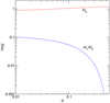 |
Fig. B.2 Log–log plot of H0 and − H1∕H0 as a function of q (case α = β = 1∕2), for |
Thus, the final results for this particular case are
![\begin{eqnarray*} &&\hspace{-7pt}\left.\begin{array}{l} \mu_0(p) = H_0(q)\,p^{-1} \\ \mu'_1(p) = H_1(q)\,p^{-3/2} \\ \mu_1(p) = [H_1(q)/H_0(q)]\,p^{-1/2} \end{array}\right\} \quad (0\leq q<1/\sqrt{3}), \nonumber\\ &&\hspace{-7pt}\left.\begin{array}{l} \mu_0(p) = 2B_0\,p^{-1} \\ \mu'_1(p) = \mu_1(p)=0 \end{array}\right\} \quad (1/\sqrt{3}\leq q<1), \\ &&\hspace{-7pt}\begin{array}{l} \mu_0(p) = \mu'_1(p) = \mu_1(p) =0 \end{array} \quad (q\ge1), \nonumber \end{eqnarray*}](/articles/aa/full_html/2019/06/aa34998-18/aa34998-18-eq190.png) (B.31)
(B.31)
where B0 is given by Eq. (A.40), H0 and H1 (see Fig. B.2) are given by
![\begin{eqnarray*} H_0(q) &=& 2B_0+[q(1-q^2)]^{1/2}({q'}^{1/2}-q^{1/2})-G_0(q)+G_0(q'),\nonumber \\ H_1(q) &=& \frac{q}{2}(1-q^2)({q'}^{1/2}-q^{1/2})-G_1(q)+G_1(q'), \end{eqnarray*}](/articles/aa/full_html/2019/06/aa34998-18/aa34998-18-eq191.png) (B.32)
(B.32)
q′ is given by Eq. (B.30), G0 is given by Eq. (A.38), and G1 results in
 (B.33)
B.6 Finite angular resolution (finite infall radius) for power-law indices 1/2
Although the first-order moment for a finite infall radius ri, observed with a finite angular resolution, has to be calculated numerically, we can study its value at the origin, for p = 0. The convolution of the moments μ0(p;ri) and  with a Gaussian beam of unit area and half-power beamwidth b,
 (B.34)
It is useful to use the variable s ≡ ri∕b, so that bothmoments can be expressed as
 (B.36)
The normalized first-order moment at the origin will be
 (B.38)
The asymptotic values of μ1(0;b, ri) for ri →∞ (equivalent to s≫ 1) must coincide with the expression derived with infinite infall radius (Eq. (22)). Effectively,
 (B.39)
as expected. Let us now evaluate the asymptotic expression for μ1 (0;b, ri) for b →∞ (equivalent to s ≪1). Taking into account that H0(q) = 0 for q > 1 and H1(q) = 0 for  ,
,
 (B.41)
where  and
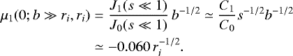
and  are constants to be evaluated numerically, resulting in C1∕C0 ≃−0.060. Thus,
 (B.42)
Appendix C Finite spectral resolution and first-order moment of a line
Let I(v) be the intensity of a line as a function of radial velocity. We are interested in calculating the first-order moment of the line profile,
 (C.1)
(C.1)
We will make use of the relationship between the zeroth and first-order moments of a function f and the values of its Fourier transform F[f] and its derivative F′[f] at the origin (see Bracewell 2000, Chap. 8)
, \quad \mu'_1= \frac{{\mathbf{F'}}[f](0)}{-2\pi i}. \end{equation*}](/articles/aa/full_html/2019/06/aa34998-18/aa34998-18-eq208.png) (C.3)
(C.3)
Let us assume that the finite spectral resolution of the spectrometer can be represented by the convolution of the real line profile with an instrumental response function W(v),
 (C.4)
(C.4)
and that the instrumental response is normalized to unit area, and is symmetric with respect to velocity or, more precisely, with zero first-order moment,
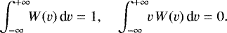 (C.5)
(C.5)
In the Fourier domain we have
=1, \quad \frac{{\mathbf{F'}}[W](0)}{-2\pi i}=0. \end{equation*}](/articles/aa/full_html/2019/06/aa34998-18/aa34998-18-eq211.png) (C.6)
(C.6)
The zeroth-order moment calculated from the observed profiles will be
 = {\mathbf{F}}[I](0)\,{\mathbf{F}}[W](0)= {\mathbf{F}}[I](0)= \mu_0, \end{equation*}](/articles/aa/full_html/2019/06/aa34998-18/aa34998-18-eq212.png) (C.7)
(C.7)
where we used that the Fourier transform of a convolution is the product of Fourier transforms (Bracewell 2000). Thus, the zeroth-ordermoment is independent of the spectral resolution.
Let us consider now the unnormalized first-order moment,
 (C.8)
(C.8)
By using the relations with the derivative of the Fourier transform, we obtain
}{-2\pi i} = \frac{({\mathbf{F}}[I]\,{\mathbf{F}}[W])'(0)}{-2\pi i} = \frac{{\mathbf{F'}}[I](0)}{-2\pi i}{\mathbf{F}}[W](0) \nonumber\\&& +\, {\mathbf{F}}[I](0)\frac{{\mathbf{F'}}[W](0)}{-2\pi i}= \frac{{\mathbf{F'}}[I](0)}{-2\pi i} = \mu'_1. \end{eqnarray*}](/articles/aa/full_html/2019/06/aa34998-18/aa34998-18-eq214.png) (C.9)
(C.9)
Thus,  is independent of the spectral resolution, and so is the normalized first-order moment,
  .
.
In conclusion. the spectral resolution does not affect the value of the first-order moment of a line, as long as the spectrometer response can be described as a convolution with an instrumental response symmetric with respect to velocity.
Appendix D 2D Convolution of a power-law function with a Gaussian beam
Let F(p) be a 2D power-law function of the radial distance
 (D.1)
(D.1)
that has to be convolved with a Gaussian beam of unit area and half-power beamwidth b,
 (D.2)
(D.2)

will have a different behavior for p ≫ b and p ≪ b. On the one hand, for p ≫ b the convolution with the Gaussian beam will not modify noticeably the power-law function and the result will not depend on b,
 (D.4)
(D.4)
On the other hand, for p ≪ b, Fb will not depend much on p and will be approximately constant,
 (D.5)
(D.5)

The integral can be evaluated analytically and the result is
 (D.7)
(D.7)
For the cases of interest, we have
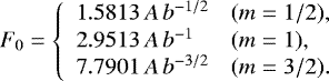 (D.8)
(D.8)
The characteristic radius that separates the two regions of Fb can be estimated as the intersection of the two asymptotic values, that is, F(pc) = F0, resulting in
![\begin{equation*} p_c= \frac{b}{(4\ln2)^{1/2}[\Gamma(1-m/2)]^{1/m}}. \end{equation*}](/articles/aa/full_html/2019/06/aa34998-18/aa34998-18-eq225.png) (D.9)
(D.9)
For the cases of interest, we have
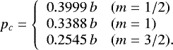 (D.10)
References
- Anglada, G., Rodríguez, L. F., Cantó, J., Estalella, R., & López, R. 1987, A&A, 186, 280 [NASA ADS] [Google Scholar]
- Anglada, G., Estalella, R., Rodríguez, L. F., Cantó, J., & López, R. 1991, A&A, 252, 639 [NASA ADS] [Google Scholar]
- Anglada, G., Rodríguez, L. F., Girart, J. M., Estalella, R., & Torrelles, J. M. 1994, ApJ, 420, L91 [NASA ADS] [CrossRef] [Google Scholar]
- Beltrán, M. T., Cesaroni, R., Neri, R., et al. 2005, A&A, 435, 901 [NASA ADS] [CrossRef] [EDP Sciences] [Google Scholar]
- Bracewell, R. N. 2000, The Fourier Transform and its Applications, 3rd edn. (Singapore: McGraw-Hill) [Google Scholar]
- Cesaroni, R., Churchwell, E., Hofner P., Walmsley, C. M., & Kurtz, S. 1994, A&A, 288, 903 [NASA ADS] [Google Scholar]
- Di Francesco, J., Myers, P. C., Wilner, D. J., Ohashi, N., & Mardones, D., 2001, ApJ, 562, 770 [NASA ADS] [CrossRef] [Google Scholar]
- Estalella, R. 2017, PASP, 129, 025003 [NASA ADS] [CrossRef] [Google Scholar]
- Estalella, R., Mausberger, R., Torrelles, J. M., et al. 1993, ApJ, 419, 698 [NASA ADS] [CrossRef] [Google Scholar]
- Evans, N. J., Di Francesco, J., Lee, J.-E., et al. 2015, ApJ, 814, 22 [CrossRef] [Google Scholar]
- Girart, J. M., Beltrán, M. T., Zhang, Q., Rao, R., & Estalella, R. 2009, Science, 324, 1408 [NASA ADS] [CrossRef] [PubMed] [Google Scholar]
- Kurono, Y., Saito, M., Kamazaki, T., Morita, K.-I., & Kawabe, R. 2013, ApJ, 765, 85 [Google Scholar]
- Juárez, C., Liu, H. B., Girart, J. M., et al. 2019, A&A, 621, A140 [NASA ADS] [CrossRef] [EDP Sciences] [Google Scholar]
- Keto, E. R., Ho, P. T. P., & Haschick, A. D. 1987, ApJ, 318, 712 [NASA ADS] [CrossRef] [Google Scholar]
- Klaassen, P. D., & Wilson, C. D. 2007, ApJ, 663, 1092 [NASA ADS] [CrossRef] [Google Scholar]
- Larson, R. B. 1972, MNRAS, 157, 121 [NASA ADS] [Google Scholar]
- Mayen-Gijon, J. M. 2015, Ph.D. Thesis, University of Granada, Granada, Spain [Google Scholar]
- Mayen-Gijon, J. M., Anglada, G., Osorio, M., et al. 2014, MNRAS, 437, 3766 [NASA ADS] [CrossRef] [Google Scholar]
- Olofsson, S., & Olofsson, G. 2009, A&A, 498, 455 [NASA ADS] [CrossRef] [EDP Sciences] [Google Scholar]
- Osorio, M., Anglada, G., Lizano, S., & D’Alessio, P. 2009, ApJ, 694, 29 [NASA ADS] [CrossRef] [Google Scholar]
- Purcell, C. R., Balasubramanyam, R., & Burton, M. G. 2006, MNRAS, 367, 553 [NASA ADS] [CrossRef] [Google Scholar]
- Salpeter, E. E. 1955, ApJ, 121, 161 [Google Scholar]
- Sepúlveda, I., Anglada, G., Estalella, R., et al. 2011, A&A, 527, A41 [NASA ADS] [CrossRef] [EDP Sciences] [Google Scholar]
- Shu, F. H. 1977, ApJ, 214, 488 [NASA ADS] [CrossRef] [Google Scholar]
- Shu, F. H., Adams, F. C., & Lizabo, S. 1987, ARA&A, 25, 23 [Google Scholar]
- Szymczak, M., Bartkiewicz, A., & Richards, A. M. S. 2007, A&A, 468, 617 [NASA ADS] [CrossRef] [EDP Sciences] [Google Scholar]
- Yang, J., Umemoto, T., Iwata, T., & Fukui, Y. 1991, ApJ, 373, 137 [NASA ADS] [CrossRef] [Google Scholar]
- Yen, H.-W., Takakuwa, S., Koch, P. M., et al. 2015, ApJ, 812, 129 [NASA ADS] [CrossRef] [Google Scholar]
- Wu, J., Sridharam, T., Fuller, G. A., Zhang, Q., & Evans, N. J. 2007, BAAS, 39, 881 [NASA ADS] [Google Scholar]
- Zhang, Q., Ho, P. T. P., & Ohashi, N. 1998, ApJ, 494, 636 [NASA ADS] [CrossRef] [Google Scholar]
- Zhou, S., Evans, N. J., II, Kompe, C., & Walmsley, C. M. 1994, Astronomy with Millimeter and Submillimeter Wave Interferometry, IAU Colloq. 140, ASP Conf. Ser., 59, 226 [NASA ADS] [Google Scholar]
All Figures
|
Fig. 1 Intersection of the surfaces of equal line-of-sight (LOS) velocity, vz, for a collapsing protostellar core, with the plane (p, z) (see Sect. 2). The LOS-velocities are different pairs of negative and positive velocities (vz = ±2−1∕2, ±1, ±21∕2, ±2). The blue lines are the contours for vz < 0, and the red lines for vz > 0. The observer, located to the right, at p = 0, z = −∞, sees the emission coming from the part of the surfaces of equal LOS-velocity facing the observer, traced with thick lines. The dashed lines indicate the position of (zm, pm) for each contour, where pm is the maximum value of p, and zm the corresponding value of z. The square frame is drawn at p = ±1, z = ±1. |
| In the text | |
|
Fig. 2 Intensity maps for pairs of LOS-velocities, Vz = ±0.8 km s−1 (top), ± 1.1 km s−1 (middle), and ± 1.4 km s−1 (bottom), calculated for a a mass M* = 1 M⊙, a distance of 140 pc, and a beam of 0.′′1. The axes are position offsets labeled in arcsec. The intensity scale is the same for all maps. We note the sharp peak at the center of the blueshifted LOS-velocity maps (left), and the flat, slightly concave shape of the redshifted LOS-velocity maps (right), and the more compact emission for high values |Vz | (bottom) than for low values of |Vz| (top). |
| In the text | |
|
Fig. 3 Intensity profiles t(p) for vz = −1 (top panel, blue) and vz = +1 (bottom panel, red). The different dashed lines indicate the blue and red wing temperature at the maximum value of p, p = pm, and the blue wing asymptotic behavior for p ≪ 1. |
| In the text | |
|
Fig. 4 Intensity profiles t(p) for pairs of positive and negative velocities, vz = ±1, ±21∕2, ±2. |
| In the text | |
|
Fig. 5 Line profile showing the emission at a projected distance p as a function of LOS velocity. The blue wing emission encompasses LOS velocities from − vm to 0, and its peak value (at vz = 0) is t2 = p−1∕2. The red wing emission encompasses LOS velocities from 0 to vm = 0.620 p−1∕2, and its peak value (at vz = vm) is t1 = 0.760 p−1∕2. |
| In the text | |
|
Fig. 6 Line profiles for values of p = 1, 21∕2, 2. |
| In the text | |
|
Fig. 7 Log–log plot of the moments μ0 and − μ1, as a functionof projected distance p. |
| In the text | |
|
Fig. 8 Log–log plots of the moments μ0 and − μ1 (solid lines) for a Gaussian beam with HPBW b = 1 (dotted line), as a function of the projected distance p, and their asymptotic values (dashed lines) for p ≪ b and p ≫ b. |
| In the text | |
|
Fig. 9 For a given projected distance |
| In the text | |
|
Fig. 10 Line profile for |
| In the text | |
|
Fig. 11 Log–log plot of μ0 and − μ1 as a functionof the projected distance p, for an infall radius ri = 1 (solid lines) and for an infinite infall radius (dashed lines). |
| In the text | |
|
Fig. 12 Log–log plot of μ0 and − μ1 as a functionof the projected distance, for an infall radius ri = 1 and beamwidth b = 0.1 in reduced units (solid lines) and b = 0 (dashed lines). |
| In the text | |
|
Fig. 13 First-order moment μ1 for an infinite infall radius, as a function of the projected distance, D θ (in kau), for beamwidths D θb = 0.1, 0.2, 0.5, 1, 2, 5, and 10 kau, where D is the distance to the source. The vertical axis scales as |
| In the text | |
|
Fig. 14 First-order moment μ1 for an infinite infall radius, as a function of the projected distance in units of the beamwidth, θ∕θb (adimensional), for central masses M* = 0.1, 0.2, 0.5, 1, 2, 5, and 10 M⊙. The vertical axis scales as |
| In the text | |
|
Fig. 15 First-order moment μ1, as a functionof projected distance in units of the infall radius, D θ∕Ri (adimensional), for beamwidths D θb = 0, 0.1, 0.2, 0.5, 1, and 2 kau, where D is the distance to the source. The vertical axis scales as |
| In the text | |
|
Fig. 16 Same as Fig. 15, for D θb = 0.1 kau, and Ri = 0.2, 0.5, 1, 2, 5, 10, and ∞ kau. The horizontal axis is the projected distance, D θ (in kau). Note that the line for Ri = 1 kau in this figure coincides with the line for D θb = 0.1 kau in Fig. 15. |
| In the text | |
|
Fig. 17 Function J(s) in the expression of μ1(0;θb, Ri), showing its asymptotic values for s ≪ 1 and s ≫ 1. |
| In the text | |
|
Fig. 18 Maps of G31 first-order (color scale) and zeroth-order moment (contours) for the ammonia inversion transitions (2, 2) to (6, 6) (Mayen-Gijon et al. 2014). The color scale, the same for all panels, ranges from 94 to 101 km s−1. The contours are in steps of 10% of the peak value for all the maps, except for the (4, 4) transition, for which the steps are 20%. The beam is shown in the lower right corner of each panel. |
| In the text | |
|
Fig. 19 G31 first-order moment for the ammonia inversion transitions (2, 2) (black line and open circles), (3, 3) (red line andfilled circles), (4, 4) (blue line and filled squares), (5, 5) (magenta line and open squares), and (6, 6) (green line and filled diamonds) (Mayen-Gijon et al. 2014), as a function of angular distance, measured for rings of width 0.′′ 1 and average radius θ. The error bars are the rms of the velocity inside each ring. The right-hand vertical axis shows the velocities obtained from the first-order moment maps, while the left-hand vertical axis shows the velocity with respect to the systemic velocity of G31, taken as V sys = 97.4 km s−1. |
| In the text | |
|
Fig. 20 Model (black dashed line) fitted to the G31 first-order moment, calculated for a central mass of 122 M⊙, an infall radius of 5 kau, and a half-power beamwidth of ~0.′′33 for the (3, 3), (5, 5), and (6, 6) transitions (top), and 0.′′16 for the (4, 4) transition (bottom). |
| In the text | |
|
Fig. 21 B335 zeroth-order (contours) and first-order moment (color scale) of the H13 CO+ (J = 1–0) line, obtained from the channel maps of Kurono et al. (2013). Contours are in steps of 511 mJy beam−1 km s−1. The color scale at the right border is in m s−1. The (0, 0) position corresponds to α(J2000) = 19h37m00.s89, δ(J2000) = +07°34′09.′′6. The synthesized beam is shown in the lower left corner. |
| In the text | |
|
Fig. 22 B335 first-order moment of the 13CO (J = 2–1) line observed with ALMA. Top: moment of the red channels, with velocities higher than the systemic velocity, V sys (color scale: 8.9–10.1 km s−1). Middle: moment of all the channels (color scale: 7.4–9.2 km s−1). Bottom: moment of the blue channels, with velocities lower than V sys (color scale: 6.8–8.0 km s−1). The (0, 0) position, marked with a plus sign, is the same as in Fig. 21. The synthesized beam is shown in the lower left corner of the middle panel. |
| In the text | |
|
Fig. 23 Same as Fig. 19 for B335. Top: H13CO+ (J = 1–0) line observed at Nobeyama (2″ ring width). Bottom: 13CO (J = 2–1) line observed with ALMA (0.′′1 ring width; |
| In the text | |
|
Fig. 24 NH3 (1, 1) line central velocity of the Guitar Core in L1287. The central blue spot is blueshifted ~ 0.5 km s−1 with respect to the ambient gas. The embedded sources in the center are indicated by dots (mm, Juárez et al. 2019), and crosses (cm, Anglada et al. 1994). The synthesized beam is shown in the lower-right corner of the map. |
| In the text | |
|
Fig. 25 Same as Fig. 19 for the Guitar Core in L1287, for the NH3 (1, 1) (blue circles)and (2, 2) lines (red circles). The rings used were 1″ wide, and a systemic velocity V sys = −18.55 km s−1 was adopted. The best fit was obtained for an infinite infall radius, and a central mass M* = 4.4 M⊙ (black dashed line). |
| In the text | |
|
Fig. B.1 Plot of q′ as a functionof q (case α = β = 1∕2), for |
| In the text | |
|
Fig. B.2 Log–log plot of H0 and − H1∕H0 as a function of q (case α = β = 1∕2), for |
| In the text | |
Current usage metrics show cumulative count of Article Views (full-text article views including HTML views, PDF and ePub downloads, according to the available data) and Abstracts Views on Vision4Press platform.
Data correspond to usage on the plateform after 2015. The current usage metrics is available 48-96 hours after online publication and is updated daily on week days.
Initial download of the metrics may take a while.