| Issue |
A&A
Volume 625, May 2019
|
|
|---|---|---|
| Article Number | A102 | |
| Number of page(s) | 20 | |
| Section | Extragalactic astronomy | |
| DOI | https://doi.org/10.1051/0004-6361/201935437 | |
| Published online | 21 May 2019 | |
MUSE unravels the ionisation and origin of metal-enriched absorbers in the gas halo of a z = 2.92 radio galaxy⋆
1
European Southern Observatory, Karl-Schwarzschild-Str. 2, 85748 Garching bei München, Germany
e-mail: skolwa@eso.org
2
Centro de Astrobiologia (CSIC-INTA), Carretera de Ajalvir, km 4, 28850 Torrejon de Ardoz, Madrid, Spain
3
Astro-UAM, UAM, Unidad Asociada CSIC, Facultad de Ciencias, Campus de Cantoblanco, 28049 Madrid, Spain
4
Instituto de Astrofísica e Ciências do Espaço, Universidade do Porto, CAUP, Rua das Estrelas, Porto 4150-762, Portugal
5
Max-Planck-Institut für Astrophysik, Karl-Schwarzschild-Str. 1, 85741 Garching bei München, Germany
6
Centre for Extragalactic Astronomy, Department of Physics, Durham University, South Road, Durham DH1 3LE, UK
7
Institut d’Astrophysique de Paris, UMR 7095, CNRS, Université Pierre et Marie Curie, 98bis boulevard Arago, 75014 Paris, France
8
International Centre for Radio Astronomy Research, Curtin University, 1 Turner Avenue, Bentley, Western Australia 6102, Australia
9
Dunlap Institute for Astronomy & Astrophysics, 50 St. George Street, Toronto, ON M5S 3H4, Canada
Received:
8
March
2019
Accepted:
9
April
2019
We have used the Multi-Unit Spectroscopic Explorer (MUSE) to study the circumgalactic medium (CGM) of a z = 2.92 radio galaxy, MRC 0943−242 by parametrising its emitting and absorbing gas. In both Lyα λ1216 and He II λ1640 lines, we observe emission with velocity shifts of Δv ≃ −1000 km s−1 from the systemic redshift of the galaxy. These blueshifted components represent kinematically perturbed gas that is aligned with the radio axis, and is therefore a signature of jet-driven outflows. Three of the four known Lyα absorbers in this source are detected at the same velocities as C IV λλ1548, 1551 and N V λλ1239, 1243 absorbers, proving that the gas is metal-enriched more so than previously thought. At the velocity of a strong Lyα absorber which has an H I column of NH I/cm−2 = 1019.2 and velocity shift of Δv ≃ −400 km s−1, we also detect Si II λ1260 and Si II λ1527 absorption, which suggests that the absorbing gas is ionisation bounded. With the added sensitivity of this MUSE observation, we are more capable of adding constraints to absorber column densities and consequently determining what powers their ionisation. To do this, we obtain photoionisation grid models in CLOUDY which show that AGN radiation is capable of ionising the gas and producing the observed column densities in a gas of metallicity of Z/Z⊙ ≃ 0.01 with a nitrogen abundance a factor of 10 greater than that of hydrogen. This metal-enriched absorbing gas, which is also spatially extended over a projected distance of r ≳ 60 kpc, is likely to have undergone chemical enrichment through stellar winds that have swept up metals from the interstellar-medium and deposited them in the outer regions of the galaxy’s halo.
Key words: galaxies: active / galaxies: individual: MRC 0943−242 / galaxies: halos / ISM: jets and outflows
The reduced datacube is only available at the CDS via anonymous ftp to cdsarc.u-strasbg.fr (130.79.128.5) or via http://cdsarc.u-strasbg.fr/viz-bin/qcat?J/A+A/625/A102
© ESO 2019
1. Introduction
High-redshift radio galaxies (HzRGs) host very powerful active galactic nuclei (AGN) and occupy the upper echelons of stellar-mass distributions for galaxies across cosmic time (Jarvis et al. 2001; De Breuck et al. 2002; Rocca-Volmerange et al. 2004; Seymour et al. 2007). They are often enshrouded by giant Lyα emitting haloes that cover regions extending out to ≥100 kpc in projection (e.g. Baum et al. 1988; Heckman et al. 1991; van Breugel et al. 2006; McCarthy et al. 1990a; van Ojik et al. 1996). These massive haloes also tend to have filamentary and clumpy sub-structures within them (Reuland et al. 2003).
In some HzRGs, extended low surface brightness haloes are found to have quiescent kinematics with line widths and velocity shifts in the order of a few 100 km s−1 (Villar-Martín et al. 2003). In the high surface brightness regions of these nebulae, however, perturbed gas kinematics with line widths and velocity shifts that are > 1000 km s−1 are frequently seen in the extended emission line region (EELR; e.g. McCarthy et al. 1996; Rottgering et al. 1997; Villar-Martín et al. 1999a). Given the alignment of the radio axis with the turbulent kinematics, this has often been interpreted as evidence for jet-gas interactions (e.g. Humphrey et al. 2006; Morais et al. 2017; Nesvadba et al. 2017a,b). For these reasons, HzRGs are generally considered some of the best laboratories for studying ionisation and kinematics of gas and of the mechanisms that power various physical processes.
These processes include accretion, ionised gas outflows, chemical enrichment, and recycling of metal-enriched material. Mechanisms of this kind have either been observed or predicted to occur within the circumgalactic medium (CGM; see Tumlinson et al. 2017 for a formal review). We can find evidence for this within the halo gas surrounding HzRGs, which comprises both the interstellar-(ISM) and the CGM. The latter is our main focus because it is the gas interface that bridges the gap between the local ISM of a galaxy and the intergalactic medium (IGM) surrounding it.
Gas inflows into the CGM have been observed in the form of accretion of IGM gas along the large-scale filaments into the halo gas of quasars and HzRGs (e.g. Vernet et al. 2017; Arrigoni Battaia et al. 2018). They have also been seen as what may possibly be gas being expelled from the ISM in the form of AGN-driven outflows or negative feedback (e.g. Holt et al. 2008; Reuland et al. 2007; Nesvadba et al. 2008; Bischetti et al. 2017). Moreover, numerous detections of diffuse, ionised gas around powerful radio galaxies have also been made in observations of ISM and CGM gas (e.g. Tadhunter et al. 1989; McCarthy et al. 1990b; Pentericci et al. 1999; Gullberg et al. 2016 is G16 from hereon). The infall of recycled gas back into the ISM, on the other hand, has been predicted by simulations (e.g. Oppenheimer & Davé 2008; Oppenheimer et al. 2010, 2018) and observed within the haloes of powerful HzRGs (e.g., Humphrey et al. 2007; Emonts et al. 2018).
The CGMs of HzRGs are multi-phase, consisting of ionised, neutral, and molecular gas. The ionised gas is often located within the EELR, where it has been heated and ionised by star-formation, jet-driven shocks, and the AGN, emitting rest-frame ultraviolet (UV)/optical photons (e.g. Villar-Martin et al. 1997; De Breuck et al. 1999, 2000; Best et al. 2000; Vernet et al. 2001; Binette et al. 2003; Villar-Martín et al. 2007; Humphrey et al. 2008a). Molecular gas, however, which is often considered a tracer for star-formation, is detected at millimeter to sub-millimeter wavelengths (Emonts et al. 2015). The neutral hydrogen component of the CGM can be parametrised by tracing Lyα emission and absorption when H I cannot be directly detected through the 21 cm line (e.g. Barnes et al. 2014).
In the Lyα lines that are detected within HzRGs haloes, the absorption line spectrums are superimposed onto the often bright Lyα emission line profiles (e.g. Rottgering et al. 1995). To quantify the absorption in the gas, standard line-fitting routines are invoked. With these, the H I gas causing resonant scattering or absorption of Lyα emission can be parametrised in terms of its kinematics and column densities. Studies using this method have found an anti-correlation between the radio sizes of HzRGs and the measured H I column densities of the absorbers, which tend to be primarily blueshifted relative to the systemic velocity of a source (van Ojik et al. 1997), which is also observed in Lyα blobs surrounding star-forming galaxies (Wilman et al. 2005). Furthermore, Wilman et al. (2004) have shown that Lyα absorbers in HzRGs generally exist in one of two forms. They are either weak absorbers with column densities ranging from NH I/cm−2 ≃ 1013−1015 and possibly form part of the Lyα forest, or they are strong absorbers with NH I/cm−2 ≳ 1018 that form behind the bow shocks of radio jets, undergoing continual fragmentation as the jet propagates (Krause 2002, 2005).
Evidence of Lyα absorption is seen both in alignment with the radio jets and at larger angles from it, proving that H I absorbing gas can be very extended, covering almost the entire extended emission line region of an HzRG (Humphrey et al. 2008b; Swinbank et al. 2015; Silva et al. 2018a,b is S18 from hereon). Such absorbers are thought to be shells of extended gas intercepting radiation from the EELR (Binette et al. 2000). In these gas shells, C IV absorption has also been detected, indicating that they have been metal enriched. Often, C IV column densities are found to be similar in magnitude to those of weak Lyα absorbers (Villar-Martín et al. 1999b; Jarvis et al. 2003; Wilman et al. 2004). In addition to being enriched with metals, results from spectro-polarimetry have suggested that at least some of these type of absorbers also contain dust (Humphrey et al. 2013).
The subject of this work, MRC 0943−242, is an HzRG at z = 2.92 that has a distinct Lyα profile featuring four discrete absorption troughs, first revealed by long-slit high-resolution spectroscopy (Rottgering et al. 1995). At even higher resolutions, the four discrete Lyα absorbers initially detected have been confirmed, and evidence for an asymmetric underlying Lyα emission profile has also being reported (e.g. Jarvis et al. 2003; Wilman et al. 2004; S18). Three of the Lyα absorbers fall into the class of weak absorption-line gas as defined by Wilman et al. (2004), while one of the Lyα absorbers has an unusually high H I column density of ∼1019 cm−2.
MUSE (Multi-unit Spectroscopic Explorer) observations of the source have provided a spatially resolved view of the variation in the Lyα line and have shown that the strong Lyα absorber in this source is extended to radial distances of r ≳ 65 kpc from the nucleus (e.g. G16). Furthermore, S18 showed that degeneracy between H I column density and Doppler parameter suggests an alternative H I column density solution of the strongest absorber, that is, NH I/cm−2 = 1015.2. In the same study, the velocity gradient of this absorber shows evidence for it being in outflow, giving credence to the idea that it formed from an early feedback mechanism (Binette et al. 2000; Jarvis et al. 2003).
These studies show that the high H I column density absorber, in particular, is a low-metallicity (i.e. Z/Z⊙ ≃ 0.0−0.02) gas shell that may have been ejected by previous AGN activity. With respect to the ionisation of the absorber, stellar photoionisation has been said to power the strong Lyα absorber (Binette et al. 2006). However, much of the progress that has made in determining the ionising mechanism for the absorbers has been hampered by the fact that only column densities of H I and C IV were available at the time. As discussed by Binette et al. (2006), constraints from other lines such as N V are needed to draw stronger conclusions about the source of ionisation and the chemical enrichment history of the gas.
In this work, we place additional constraints on absorption in C IV, N V, and Si IV. This is possible with MUSE, which has the sensitivity and spatial resolution needed to measure the size, mass, and kinematics of both the emitting and absorbing gas around HzRGs (e.g. Swinbank et al. 2015; G16; S18). Both G16 and S18 used the MUSE commissioning data, which had an on-target time of 1 h. The observations used in this work were obtained over a 4 h on-source integration time and thus have detections with a higher signal-to-noise ratio (S/N) of the rest-frame UV lines. Hence, we have been able to detect absorption in resonance lines of lower surface brightness than Lyα and C IV, which both G16 and S18 have previously studied using MUSE data.
The paper is structured in the following way. We provide an outline of the data acquisition and reduction steps in Sect. 2. Section 3 is dedicated to explaining the details behind the line-fitting routine. In Sect. 4 we present the line models for the emitting and absorbing gas components. In Sect. 5 we describe the size, shape, and mass and give the ionised fraction of the strongest Lyα absorber. The column densities of absorbers in MRC 0943−242 are compared to quasar absorbers in Sect. 7. We use photoionisation models to assess whether the AGN can ionise the absorbers to match the observed chemical abundance levels in Sect. 8. We provide an interpretation of our results in Sect. 9 and summarise the main findings in Sect. 10.
Throughout the paper, we use ΛCDM results from the Planck 2015 mission, that is, H0 = 67.8 km s−1 Mpc−1, ΩM = 0.308 (Planck Collaboration XIII 2016). At the redshift of the galaxy, z = 2.92, a projected distance of 1″subtends a distance of 7.95 kpc.
2. Observations and data reduction
2.1. MUSE
MUSE observations were carried out on the Very Large Telescope (VLT) from 2015 December 14 to 2015 December 15 and from 2016 January 14 to 2016 January 18 UT. For the radio galaxy studied in this paper, MRC 0943−242, the observations were obtained under the program run 096.B-0752(A) (PI: Vernet). In the extended wide-field mode, MUSE observes over a wavelength range of λ = 4650−9300 Å without the use of adaptive optics (WFM-NOAO-E). The instrument resolving power is λ/Δλ = 1700−3400, which corresponds to a spectral resolution of Δλ = 2.82−2.74 Å or Δv ∼ 180−90 km s−1 (ranging from blue to red). MUSE has a spectral binning of 1.25 Å pix−1 and field of view (FOV) that is 1 × 1 arcmin2, with a spatial sampling of 0.2 × 0.2 arcsec2 (Bacon et al. 2014).
Observations of the target, MRC 0943−242, were obtained over 8 × 30 min observing blocks (OBs) amounting to 4 h of on-source time. The average seeing disc diameter for the run, under clear conditions, is estimated to be FWHM = (0.74 ± 0.04)″. We reduced the raw data in ESOREX using the MUSE Data Reduction Software (MUSE DRS) pipeline, version 1.6.2 (Weilbacher et al. 2014). The data were subsequently processed with the standard MUSE reduction recipe, and individual OB exposures were combined at the end of the procedure to create the final datacube (available at the CDS).
Sky subtraction of the data was performed using the principal component analysis (PCA) algorithm, Zurich Atmosphere Purge (ZAP), which was developed for use on MUSE data (Soto et al. 2016). After a coarse sky subtraction is carried out, the PCA removes sky residuals that result from spaxel to spaxel (spatial pixel) variations in the line spread function.
The MUSE astrometry loses precision due to instrument effects, hence we added a slight correction to the astrometry of the final datacube. This was done by identifying field stars in the MUSE FOV from the Gaia DR2 (Data Release 2) catalogue (Gaia Collaboration 2016, 2018) and computing their astrometry offsets from the Gaia DR2 frame. We calculated these offsets for eight field stars and used the average right-ascension and declination shifts to reset the central pixel co-ordinates in the MUSE cube header, which made the MUSE co-ordinate frame more accurate.
2.2. UVES
To supplement this study, we have obtained ancillary data from the VLT instrument, the Ultraviolet Echelle Spectrograph (UVES; D’Odorico et al. 2000; Dekker et al. 2000). These observations show the Lyα line in the spectrum of MRC 0943−242 (Jarvis et al. 2003; Wilman et al. 2004; S18). During this 3.4 h observation, the red arm of the instrument was used and the configuration was set to a central wavelength of 5800 Å. The widths of the spatial and spectral binning were 0.5″ and 0.05−0.06 Å. The observing conditions resulted in an average seeing disc of 0.8″. The data were reduced using IRAF, invoking the standard recipe for echelle spectroscopic data outlined in Churchill (1995).
To obtain the archival 1D spectrum used in this work, the slit was positioned at an angle of 74° east of north with a width of 1.2″, length of 5″ that covered all of the emission from the brightest regions of the gas halo. The spectral resolution ranged between 25 000−40 000 or 12−8 km s−1, ranging from blue to red.
UVES is better able to resolve the most narrow absorption lines because of its very high spectral resolution. Narrow lines are broadened by instruments, such as MUSE, that have moderate spectral resolution. Hence, the UVES data serve the purpose of allowing us to check the validity of the spectral line-fitting that we perform.
3. Spectrum extraction and line-fitting method
3.1. 1D spectrum extraction
With the goal of studying the absorbing gas surrounding the host galaxy of MRC 0943−242 (which we refer to as Yggdrasil, following the naming convention provided in G16), we extracted a 1D spectrum from a sight-line in the MUSE datacube where the surface brightness (SB) of rest-frame UV emission is highest. We refer to it as the high surface brightness region (HSBR) within the gas halo of Yggdrasil, which we are interested in studying (shown in Fig. 1). Although it sits within the brightest parts of the gas halo, it is not the location of the AGN because this cannot be easily inferred. From this HSBR, we extracted the 1D spectrum over an aperture with a radius of R = 3 spaxels or R = 0.6″ centred at the brightest spatial pixel or spaxel located at the co-ordinates, (α, δ) = ( ). Collapsing the sub-cube spatially by summing the flux over all spaxels, we obtained the rest-frame UV spectrum shown in Fig. 2.
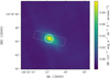 |
Fig. 1. MUSE line and continuum (white-light) image of MRC 0943−242. At the centre of the image is the high surface brightness region of the galaxy halo. The sub-cube aperture from which the spectrum in Fig. 2 is obtained is shown within the circle. The UVES slit (dotted outline) has a 1.2″ width and extends over 5″. |
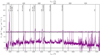 |
Fig. 2. MUSE spectrum of the high surface brightness region in the halo of MRC 0943−243. The spectrum contains several rest-frame UV lines that are labelled and indicated by the dashed vertical lines. The upper panel shows the entire flux density range for the spectrum, while the lower panel covers only the low flux density range to show the lower S/N lines more clearly. |
3.2. Line-fitting procedure
The goal of this work is to parametrise the physical conditions of gas in the halo of the radio galaxy Yggdrasil. To do this, we used the line profiles of ions that undergo resonance transitions, that is, Lyα λ1216, C IV λλ1548, 1551, N V λλ1238, 1243, and Si IV λλ1393, 1402 (see Fig. 2). We applied line-fitting procedures that combine Gaussian and Voigt models in order to characterise the emission and absorption simultaneously. The emergent emission is Fλ = Fλ, 0e−(τλ, 1 + … + τλ, n) for n absorbers, where the unabsorbed emission, Fλ, 0, is denoted by the Gaussian function
![$$ \begin{aligned} F_{\lambda ,0} = \frac{ F }{ \sigma _\lambda \sqrt{2\pi }} \exp \left[{-\frac{1}{2}\left(\frac{\lambda - \lambda _0}{\sigma _\lambda }\right)^2}\right], \end{aligned} $$](/articles/aa/full_html/2019/05/aa35437-19/aa35437-19-eq2.gif)
where F is the integrated flux of the underlying emission, λ0 is the Gaussian line centre, σλ is the line width, and λ is the wavelength. The absorption is quantified by the optical depth, τλ, which is denoted by the Voigt–Hjerting function
where N is the column density, e (electron charge), me (electron mass), and c (light speed) are fundamental constants, and f is the oscillator strength. H(a, u) is the Hjerting function in which  and
and  such that Γ is the Lorentzian width, ΔλD is the Doppler parameter (also b parameter), and λ − λ0, is the frequency shift from the line centre (λ0). H(a, u) is obtained from the Tepper-García (2006) approximation, which is well suited for absorption systems that have column densities N/cm−2 ≤ 1022. When fitting the absorption, we also made the simplifying assumption that each cloud of absorbing gas covers the emission line region with a unity covering factor (C ≃ 1.0).
We used the PYTHON package LMFIT to carry out the non-linear least-squares fitting (Newville et al. 2016). Our fitting method of choice was the Levenberg–Marquardt algorithm, which performs the χ2-minimisation that yields our best-fit results. In the figures, we report the reduced χ2-squared value,  , where N is the number of data points and Ni is the number of free parameters. For each line, we calculated the local continuum level by masking the line emission and fitting a first-order polynomial to the surrounding continuum. The first-order polynomial was subtracted from both the line and continuum of He II and Lyα, which are bright enough that not fitting the continuum has little effect on the overall fit. For C IV, N V, and Si IV, which are lower in surface brightness (than Lyα and He II), the continuum is likely to impact the overall fit.
Fitting Gaussian and Voigt functions simultaneously means that the composite model has many fit parameters. To prevent over-fitting and also to obtain a physical result, we used Lyα and He II as initial guesses when we fitted underlying emission and absorption profiles to the C IV, N V, and Si IV+O IV] lines.
From the He II fit (described later in Sect. 4.1), we obtained the best-fit results for Gaussian fluxes (Fλ), line widths (σλ), and line centres (λ0). Δλ0,He II is the error on the fitted He II line centre such that λ0,He II = 6436.09 ± 0.30 Å. The line centres are in agreement with the He II systemic velocity (or zero velocity, which is fixed to the systemic redshift of the galaxy) within its uncertainties, that is, Δλ0,He II = 0.30 Å = 10.3 km s−1, under the assumption that all the emission originates from the centre of the halo. The He II fit results for line width and the redshift of the line centre were set as initial guesses in Gaussian fits for emission in the resonant lines, C IV, N V, Si IV and the non-resonant O IV], which emits as part of the Si IV+O IV] intercombination line. Furthermore, we ensured that Fλ and σλ remain positive.
To fit the Lyα absorption in the MUSE spectrum, we used the best-fit parameters from the literature (i.e. Jarvis et al. 2003; Wilman et al. 2004) as initial guesses in the fitting procedure. The best-fit Lyα absorber redshifts were passed on as initial guesses for absorber redshifts in the C IV, N V, and Si IV line profiles. The initial guesses for column densities and Doppler parameters are based on rough estimates from the literature (i.e. Jarvis et al. 2003; Wilman et al. 2004, G16; S18). All three Voigt parameters have a limited parameter space over which a solution can be obtained. These parameter constraints are summarised in Table 1.
Lower and upper bounds placed on initial conditions in the line-fitting routine.
In the fitting routine, some absorber redshifts were given more freedom to vary over a given parameter space than others because the ionisation energies of the different gas tracers, H I, C IV, N V, and Si IV, differ greatly such that EH I = 13.6 eV, EC IV = 64.5 eV, EN V = 97.9 eV, and ESi IV = 45.1 eV. It would be unrealistic to expect them to exist at exactly the same redshifts.
The minimum Doppler parameter permissible in the line-fitting is set by the lower limit of the MUSE spectral resolution, which suggests that an approximate lower limit of bmin ∼ σλ = 90 km s−1 / 2.3548 ≃ 40 km s−1. We set a conservative upper limit of bmax = 400 km s−1 for C IV, N V, and Si IV with the understanding that the absorbing gas is kinematically quiet in relation to perturbed gas regions that have FWHM ≥ 1000 km s−1.
In general, Lyα absorbers in HzRG gas nebulae are found to have low column densities of NH I/cm−2 = 1013−1015 or be optically thick with column densities of NH I/cm−2 > 1018 (Wilman et al. 2004). Because H I is frequently more abundant than metals in halo gas environments, we can expect the column densities of the metal ions to be lower. Hence, we set the lower and upper limits for permissible fitted column densities to N/cm−2 = 1012 − 1020 cm−2. A full summary of the initial boundary conditions in the fitting procedure is given in Table 1.
4. Best-fit line models
4.1. He II
He II λ1640 is the brightest non-resonant emission line and forms the basis our estimation of the underlying emission profiles of the lines we study here, that is, Lyα, C IV, N V, and Si IV. In the extracted spectrum, we obtained a detection of He II emission that forms through cascade recombination of He++, which emits a non-resonant photon. The He II lines are often used to determine the systemic redshift of a galaxy (e.g. Reuland et al. 2007; Swinbank et al. 2015; S18). Although Lyα is brighter than He II, we refrained from using Lyα for this purpose because of its susceptibility to radiative transfer effects that clearly affect the emergent line emission.
The He II line, shown in Fig. 3, has an excess of emission at Δv ∼ −1000 km s−1 that is not present at Δv ∼ 1000 km s−1, indicating asymmetry. This has been identified before in Jarvis et al. (2003), where the excess was found to have little effect on the final fit. Our 1D spectrum has brighter line detections, and to account for the excess emission in the wing, we therefore fit the He II line with two Gaussian profiles: one for emission blueshifted relative to and another for emission originating from the systemic velocity. This method has been employed frequently for fitting asymmetric line profiles from various gas phases (e.g. Mullaney et al. 2013; Cicone et al. 2014; Rakshit & Woo 2018; Hernández-García et al. 2018; Perna et al. 2019).
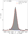 |
Fig. 3. He II λ1640 line in the MUSE spectrum (shown in Fig. 2). The line profile has been continuum subtracted. The best-fit model (red) consists of two Gaussian profiles. The first Gaussian component (in blue) models the excess blue wing emission at the negative velocities, while the second component (in orange) models the emission at the systemic velocity of the galaxy. |
We estimated the central velocity of the excess emission in He II by spatially identifying where its emission peaks in surface brightness (explained further in Sect. 6). The best-fit Gaussian parameters obtained from the spatially offset region were used to fit the blueshifted emission as a second component to the emission from the HSBR at the systemic velocity. The result of this fitting procedure is shown in Fig. 3, where the additional component is broadened to a line width of FWHM ≃ 1000 km s−1 and also blueshifted from the systemic velocity. From the He II best-fit result, we obtain a fiducial systemic redshift of zsys = 2.9235 ± 0.0001 that denotes the zero velocity for all the lines identified in Fig. 2.
4.2. H I Lyα
H I Lyα λ1216 is the brightest line in the rest-frame UV spectrum. We fit the Lyα emission envelope with a double Gaussian: one to the non-absorbed singlet emission at the line centre, and another to the strong blue wing emission at Δv ≃ −1000 km s−1 (see Fig. 4). The motivation for including a second emission component to the Lyα fit is twofold: a) it is well detected in the emission line He II and therefore likely to also emit in Lyα, and b) there is an asymmetry between emission at the blue and red wings of Lyα. Once fit, we see that including a second Gaussian improved the Lyα emission fit.
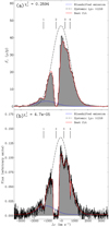 |
Fig. 4. MUSE-detected continuum-subtracted Lyα (upper panel) and ancillary UVES-detected Lyα (lower panel) for Yggdrasil. The best-fit line model (red) combines Lyα emission consisting of blueshifted and systemic components, as well as the four known absorption troughs. |
The updated Gaussian fit describes the Lyα profile well in both MUSE and UVES spectra and the best-fit parameters are in good agreement with the literature (see Tables 3 and 4). This is expected because Lyα is affected by radiative transfer effects and is therefore less likely to have a symmetric emission profile. There is also an additional underlying kinematic component causing the blue wing excess, based on the He II line fit (see Fig. 3).
To account for the absorbers, we fit four Voigt profiles, as has been done in previous works on this topic (i.e. van Ojik et al. 1997; Jarvis et al. 2003; Wilman et al. 2004; G16; B18). We also convolved the Voigt profiles with the line-spread function (LSF) of MUSE, using a fast-Fourier transform similar to that used to convolve Voigt and LSF profiles in the package, VPFIT (Krogager 2018). The LSF or instrumental profile (IP) of MUSE, when convolved with the Voigt profile, has an average Gaussian width of < σλ >= 2.65Å.
We show the line-fitting result for Lyα in Fig. 4a. Below this in Fig. 4b, we show a similar fit to the Lyα profile as was detected with UVES, which has an LSF with an average Gaussian width of < σλ >= 0.3 Å.
The Lyα absorber redshifts are used to predict the most probable redshifts for the absorbers, in general. In particular, the redshifts of the absorbers associated with resonance metal ions, C IV, N V, and Si IV, are constrained to stay within 4Δzsys (where Δzsys = 1.35 × 10⁻⁴) agreement of the measured Lyα absorber redshifts. This is done following the hypothesis that Lyα absorption occurs within roughly the same volume of gas as absorption of photons associated with the resonant transitions.
For this to occur, there would need to be a very strong ionising continuum to produce all of the observed ions, which is possible with ionisation by the AGN. The different ionisation energies also imply that fixing the absorbers to exactly the same redshift is unrealistic. This is why we allowed the fitted absorber redshifts to vary over a parameter space that depends on how tightly a parameter needed to be constrained.
4.3. C IV and N V
We have obtained detections of C IV λλ1548, 1551 and N V λλ1238, 1243. Given that Lyα absorber 4 is narrow, it is likely to suffer the highest degree of instrumental broadening in MUSE, as seen in Fig. 4a. For C IV and N V, we therefore did not include a fourth absorber in the model. At the MUSE spectral resolution we expect to lose any absorption signal from such a narrow absorber. The Voigt profiles were, as with Lyα, convolved with the LSF of MUSE.
The observed emission in the doublet lines, C IV and N V, was fit with two Gaussian functions that were constrained according to atomic physics (all constraints are summarised in Table 2). The local continuum was estimated using a separate linear polynomial fit (to the continuum only, with line emission masked). The continuum was thus fixed during fitting. Additionally, in C IV, we fit a second component to each of the doublet lines to account for the blueshifted emission seen in He II, which has a similar S/N level as C IV. N V has a lower S/N than both of these lines, therefore the blueshifted emission is likely to be negligible in this fit.
Doublet constraints, set by atomic physics, are embedded in the fitting to obtain best-fit results for C IV, N V, and Si IV+O IV].
Best-fit results to the absorbers in the UVES Lyα spectrum from this work and from Jarvis et al. (2003) and Wilman et al. (2004).
Best-fit results to the non-absorbed emission in the UVES spectrum. The flux units are arbitrary (arb.).
We obtained atomic constants such as rest wavelengths and oscillator strengths from the database provided by Cashman et al. (2017). For doublet lines, the ratios of line centres (i.e. λ1/λ2) and rest-frame wavelengths were fixed to one another. The doublet emission originates from the same gas, therefore the doublet line widths are equal, that is, σλ, 1 = σλ, 2. The doublet ratios (DR = F1/F2) were fixed to the those of the oscillator strengths such that they are DR = 2. Doublet ratios of 2 are observed frequently in quasar absorption lines. This is particularly true for C IV lines, whose doublet ratios vary from 2 to 1 from the linear to the saturated absorption regimes (Péroux et al. 2004). Assuming that C IV and N V absorbers 1 and 3 are not saturated and have a unity covering factor, C ≃ 1.0, because their emission does not reach zero flux level at the absorber velocities, we set DR = 2 when fitting.
The best-fit models for C IV and N V are shown in Figs. 5 and 6. The emission and absorption fit results are shown in Tables 5 and 6, respectively. We note that both C IV and N V fits feature a slight kink at Δv ∼ −2000 km s−1. This may be the result of the column density of absorber 1 being over-estimated at this velocity, which could imply that the blueshifted C IV emission is not impeded by absorber 1, as we have assumed. Rather, absorber 1 covers the emission line region behind it, the blueshifted emission. Determining which absorbers cover the systemic and/or the blueshifted emission is a task that will require higher spatial and/or spectral resolution. For simplicity, we assumed that all three absorbers impede the systemic, blueshifted, and continuum emission components.
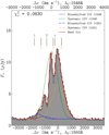 |
Fig. 5. Best-fit line model fit to C IV λλ1548, 1551 detected with MUSE. The green and orange dashed lines represent the underlying doublet emission at wavelengths of 1548 Å and 1551 Å, which are the rest-frame velocities, in the upper and lower axes, respectively. Three Voigt profiles model the absorbers for each emission line in the doublet. |
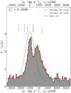 |
Fig. 6. Best-fit line model to N V λλ1238, 1242 detected with MUSE. The green and orange dashed lines represent the underlying doublet emission at the rest-frame wavelengths 1238 Å and 1242 Å, which are fixed to the systemic velocity in the upper and lower axes, respectively. Three Voigt profiles model the absorbers for each emission line in the doublet. |
Best-fit results to the absorbers in the MUSE spectrum.
Best-fit results to non-absorbed emission in the MUSE spectrum.
4.4. Si IV+O IV]
The detected Si IV λλ1393, 1402 line doublet overlaps with emission from the O IV] quintuplet. Si IV is a resonance line, and we modelled it with an absorption line at the same velocity as Lyα absorber 2. We did not include absorbers 1 and 3 because the fit did not change significantly when they were added.
As before, the Voigt profile was convolved with the LSF of MUSE and the Si IV doublet emission was modelled by two Gaussians. Again, we fixed the continuum to the result of the linear polynomial fit of the local continuum (while the line emission was masked). The O IV] quintuplet comprises five emission components at the rest-frame wavelengths for O IV], which are 1397.2 Å, 1399.8 Å, 1401.2 Å, 1404.8 Å, and 1407.4 Å. To fit these, we used five Gaussian profiles with equal line widths. The quintuplet ratios were set by the oscillator strengths of each transition. We show the fit for the intercombination Si IV+O IV] lines in Fig. 7, and the absorption fit results are shown in Table 5 and those for emission in Table 6.
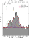 |
Fig. 7. Best fit line model to the intercombination Si IV λλ1393, 1402 + O IV] line detected with MUSE. The green and orange dashed lines represent the underlying doublet emission at the rest-frame wavelengths, 1393 Å and 1402 Å, which are fixed to the systemic velocity in the upper and low axes, respectively. The O IV] quintuplet line emission is shown in purple. |
In an attempt to confirm the consistency of this result, we compared the fluxes of the same Si IV and O IV] lines detected at high spectral resolution for the binary symbiotic star RR Telescopii, which is shown in Fig. 5 of Keenan et al. (2002). The best-fit flux ratios for O IV] are consistent with those of the high-resolution stellar spectrum, which is the perhaps the best observational comparison available for Si IV and O IV] intercombination line fluxes.
4.5. Si II
We have detected Si II λ1260 and Si II λ1527 absorption in the rest-frame UV spectrum. They were fit with Gaussians to account for the absorbed components (see Figs. 8 and 9). Using this fit, we estimated their velocity shifts and column densities using the approximation from Humphrey et al. (2008b),

where N is the column density, Wλ is the observed equivalent width, me is the electron mass, c is the light speed, e is the electron mass, f the oscillator strength, and λ0 the rest wavelength of the line. The column densities are lower limits because it is not possible to determine whether the lines are in the linear or logarithmic (flat) part of the curve of growth.
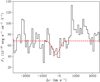 |
Fig. 8. Si II λ1260 absorption line fit with a single Gaussian component. The best-fit line is shown in red. |
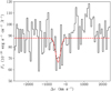 |
Fig. 9. Si II λ1527 absorption line fit with a single Gaussian component. The best-fit line is shown in red. |
The column densities of the Si II lines place them in the category of weak absorbers. Their velocity shifts are in agreement with that of Lyα absorber 2, meaning that these absorptions also occur within roughly the same gas volume as those of H I, C IV, N V, and Si IV absorbers (as Fig. 10 shows). One implication of this finding is that it is unlikely for the strong absorber to be matter bounded1. For absorber 2 to be matter bounded, low-ionisation species such as Si II would exist only in trace amounts compared to higher ionisation lines. A clear detection of both these ions at the same velocity as the strong absorber proves that the absorber is more probably ionisation bounded and has a unity covering factor. This also implies that ionising photons will not be able to escape from the CGM of this source and that ionising radiation emerging from the halo will not contribute significantly to the metagalactic background or ionisation of gas in the IGM.
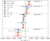 |
Fig. 10. Relative velocities of Lyα, N V, and C IV and Si II absorbers from this work as well as those from G16 and S18. The vertical dash-dotted (black) line indicates the systemic velocity and its error (shaded grey). The horizontal dotted lines (grey) distinguish between the different absorbers. |
4.6. C III] and C II]
The gas tracers C III] λλ1906, 1908 and C II] λ2326 are non-resonant lines but useful tracers when searching for evidence of shock ionisation, which we discuss in more detail in Sect. 8. We therefore included them in the line-fitting routine. To the C III] doublet, we fit four Gaussian components in total to account for emission from the doublet at both systemic and blueshifted velocities as we have done for Lyα, He II, and C IV. C III] has a sufficiently high surface brightness for us to fit it in the same way. Its best-fit result is shown in Fig. 11. C II] is a singlet that showed evidence of very blueshifted emission relative to systemic, and thus we also added an additional Gaussian component when fitting it (see Fig. 12). The best-fit emission parameters for both of these lines are shown in Table 6.
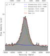 |
Fig. 11. C III] λλ1906, 1908 doublet line-fit consisting of a blueshifted emission component. |
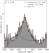 |
Fig. 12. C II] λ2326 singlet line-fit consisting of a blueshifted emission component. |
5. Morphology of the absorbers
The morphology of the absorbers within the circumgalactic medium of Yggdrasil is a focus of interest because much uncertainty about their origin and probable fate still remains, although the absorbers have been studied extensively using data from long-slit (i.e. Rottgering et al. 1995; van Ojik et al. 1997) and echelle spectroscopy (i.e. Jarvis et al. 2003; Wilman et al. 2004), which were limited in their ability to provide a spatially resolved view of the gas in emission and absorption around Yggdrasil. In particular, they were not capable of showing the spatial variation in the Lyα profile that indicates variation in the kinematics of the most extended absorber (absorber 2).
The MUSE data we used to perform resonance line-fitting above provide us with the capability of estimating the full extent and shape of Lyα absorber 2, which has a covering factor of C ≃ 1.0, as G16 and S18 have shown. Furthermore, we can deduce its neutral and also ionised gas mass, and thus estimate its total hydrogen gas mass.
5.1. Size, shape, mass, and ionisation of the strongest Lyα absorber
In agreement with previous work on the Lyα line in Yggdrasil, absorber 2, located at a velocity shift of Δv ∼ −400 km s−1, reaches zero flux at its line centre. This implies that it is saturated with a unity covering factor, that is, C ≃ 1.0 and Lyα column density of ∼1019 cm−2 (see Table 5). In the UVES spectrum, the Lyα absorbers occupy disparate velocities. This implies that the structure of the H I gas is likely to be shell-like, as Binette et al. (2000) and Jarvis et al. (2003) have suggested. Guided by these previous findings and using more recent IFU data, we can estimate the size, shape, and mass of absorber 2, which is the strongest Lyα absorber.
In terms of location, we relied on the result given in Binette et al. (2000), who showed that the absorbing and emitting gas are not co-spatial. Rather, absorber 2 is farther out from the halo and screens the radiation from the extended emission line region. We base the rest of our description of the halo gas on this predication. The spatial extent of the absorbing H I gas medium in Rottgering et al. (1995) is found to be r ≳ 13 kpc based on the extent of the measured Lyα emission and on the assumption of a unity covering factor for the associated absorption. In G16, visual inspection of the IFU data led to a value of r ≳ 60 kpc in radial extent. In S18, a velocity gradient across the halo was measured and used to estimate the absorber size, which the authors found to be r ≳ 38 kpc in radius. Here, we used the radial size of the H I gas shell from G16, who determined the size by pinpointing the farthest spaxels from the nucleus of the gas halo at several position angles where the Lyα absorber 2 is still observed.
In our data, we find that the absorber extends to projected distances of between r = 50 kpc and r = 60 kpc from the HSBR and is non-isotropic, covering the EELR over an area of 50 × 60 kpc2. A low surface brightness halo with quiescent kinematics (FWHM = 400−600 km s−1) extending out to r = 67 kpc has been detected in this source (e.g. Villar-Martín et al. 2003). Lyα, He II, N V, and C IV emission are detected in the giant halo. In fact, N V appears to be strengthened more than in the quiescent haloes of other HzRGs in Villar-Martín et al. (2003). Given the size of the absorber, it is likely that it covers the emission from the giant halo.
Assuming spherical symmetry and density homogeneity of the absorbing gas shell, the H I mass is estimated to be MH I = 4πr2mH INH I (De Breuck et al. 2003; Humphrey et al. 2008b). When we take into account the estimated size of r ≳ 60 kpc and an H I column density of 1019.2 cm−2 (from Table 5), the H I mass of absorber 2 is MH I/M⊙ = 5.7 × 10⁹(r/60 kpc)2 (NH I/1019.2 cm−2). Our results agree to within at most two orders of magnitude with those in the literature. Rottgering et al. (1995) estimated the mass of absorber 2 as MH I/M⊙ ≳ 2.0 × 10⁷(NH I/1019 cm−2)(r/13 kpc). In G16, this value is MH I/M⊙ ≳ 3.8 × 10⁹(r/60 kpc)2 (NH I/1019 cm−2), and the estimate given in S18 is MH I/M⊙ ≳ 108.3.
An approximation of the hydrogen ionisation fraction XH II = H II/(H I + H II) is clearly required to estimate the gas mass of the absorbing structure from our observational measurement of NH I. In principle, the value of XH II can vary from zero in the case of purely neutral gas to ∼1.0 in the case of matter-bounded photoionised gas (e.g. Binette et al. 1996; Wilson et al. 1997). In the absence of a method for directly estimating NH II, we instead turn to the carbon ionisation fraction, XC, which we define here as the ratio of all ionised species of carbon to all species of atomic carbon (i.e. ionised or neutral). For Yggdrasil, we combined the measurement of NC IV with the upper limit NC I ≤ 1.5 ×1014 cm−2 from S18 to obtain XC ≥ NC IV/(NC I + NC IV) = 0.8.
This is a lower limit because we have no useful constraints on any of the other ionised carbon species. The fact that the ionisation energy of C I (11.3 eV) is similar to that of H I (13.6 eV) means that under photoionisation, we can assume that the ionisation fraction of hydrogen and carbon are similar, that is, XH II ∼ XC, and thus we obtain XH II ≳ 0.8. This falls within the framework of the absorber being ionisation rather than matter bounded, as suggested by the Si II detections in Sect. 4.5.
The neutral fraction is what is remaining, that is, XH I ≲ 0.2. When we assume that the absorber is a two-phase medium as in Binette et al. (2000), the ionised fraction implies that MH II/MH I ≳ 4. Using this, we can estimate the total hydrogen mass (excluding the molecular gas contribution) of the absorber such that it is MT/M⊙ ≳ MH I + MH II = 5MH I, hence MT/M⊙ ≳ 2.9 × 10¹⁰. The mass of absorber 2 is approximately an order of magnitude lower than the stellar mass of the host galaxy, which is M*/M⊙ = 1.2 × 10¹¹ (Seymour et al. 2007).
5.2. Arrangement of the absorbers along the line of sight
Figure 10 shows that Lyα absorption occurs in the same gas volume as absorbers 1, 2, and 3 in C IV, N V, and Si IV. From the velocities of these absorbers, we can determine a) their geometric arrangement in the halo and b) their kinematics. Are these outflowing (e.g. Zirm et al. 2005; Nesvadba et al. 2006) or infalling gas (e.g. Barkana & Loeb 2003; Humphrey et al. 2008b)?
In agreement with general observations of HzRGs, Lyα absorbers 1 and 2 are blueshifted relative to the systemic velocity (Wilman et al. 2004). According to velocity gradient measures across the diameter of the Lyα halo in S18, Lyα absorber 2 is outflowing. Assuming that absorbers 1, 2, and 3 are outflowing, we can estimate where they are located in relation to one another along the line of sight. At Δv ∼ −1000 km s−1, absorber 1 has the highest blueshift and is thus more likely to be found at a closer proximity to the nucleus than absorber 2, which is located at Δv ∼ −400 km s−1. In other words, absorber 1 has the fastest outflow velocity and is therefore closer the centre of the halo. Absorber 3 is redshifted relative to the systemic velocity, and it may be infalling. To measure the distances, we require simulated abundances produced by photoionisation models (shown in Sect. 8).
6. Blueshifted He II, Lyα, and C IV emission
The blueshifted components in the bright lines He II, Lyα, and C IV are a clear indication of perturbed gas either in the foreground of systemic emission in the halo or outflowing along the line of sight. To separate the blueshifted and systemic emissions in He II, we used narrow-band imaging. A MUSE narrow-band image summed over a wavelength range of 6400−6425 Å is shown as contours in Fig. 13. We note that the contours are continuum-free. Within this chosen wavelength range, we obtain detections from the blueshifted and systemic He II emitters. The image clearly shows two spatially unresolved components: one at the high surface brightness peak, and the other spatially offset.
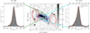 |
Fig. 13. Broad-band image of the rest-frame UV continuum of MRC 0942−242 from the HST WFPC2 702W (5800−8600 Å) filter. MUSE contours (blue) are overlaid and represent narrow-band emission summed over 6400−6425 Å. The contours are shown at the surface brightness levels, (1.0, 1.6, 2.2, 2.8, 3.4, 4.0) ×10−17 erg s−1 cm−2 arcsec−2. VLA 4.7 GHz radio surface brightness is shown by the red contour levels. The inset 1D spectra show the HSBR (left panel) and offset (right panel) He II emission. The line profiles are extracted from apertures of radius R = 0.6″, shown in green for the HSBR and in cyan for the offset region. The aperture centroids for each are shown in matching colours. The blueshifted and systemic He II emissions are shown in blue and orange, respectively, and the sum of both components is shown in red. |
In addition to this spatial separation, the He II spectra extracted from each of these two regions show that emission in the HSBR (shown in Fig. 1) is dominated by emission from the systemic velocity; trace amounts are blueshifted. The blueshifted component, however, undergoes a flux enhancement by an approximate factor of 2 (see Table 7) at a projected distance of d = 1.00 ± 0.04″ = 8.0±0.3 kpc south-west (PA ≃225°) from the HSBR.
For further understanding, we show the MUSE He II contours over a UV/optical Hubble Space Telescope (HST) Wide Field Planetary Camera 2 (WFPC2) 702W broad-band image. The UV emission detected over 5800−8600 Å appears to have a bent morphology that extends in the same direction as the region where He II is enhanced. Moreover, the UV broad-band detection and the blueshifted He II are both aligned with the radio axis detected by 4.7 GHz Very Large Array (VLA) observations (Carilli et al. 1997; Pentericci et al. 1999).
Obtaining a narrow-band image over a smaller wavelength range of 6400−6412 Å (blue interval in Fig. 14d) allows us to distinguish the blueshifted He II emission from the He II emission at the systemic velocity. He II emission from the blueshifted component alone is shown in Fig. 14a, which proves that emission from the blue wing of the He II line is indeed spatially offset from the HSBR.
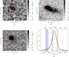 |
Fig. 14. MUSE continuum-subtracted narrow-band images showing the spatial variation in He II emission at different wavelength bands. The green and cyan crosses show the centres of the HSBR and offset He II emission from which the line profiles in Fig. 13 are extracted. The 4.7 GHz VLA radio contours are shown in red at the levels 3σ, |


THE He II emission at the systemic velocity is less highly concentrated. Over the green interval in Fig. 14d, He II is diffuse and elongated well beyond the radio lobes, indicating possible jet-gas interactions. At the red wing of the line, He II emission is concentrated in the eastern lobe and HSBR, as Fig. 14c shows.
Both Lyα and C IV show evidence for turbulent blueshifted motions in the line-fitting (see Sects. 4.2 and 4.3). If the blueshifted component is indeed an outflow, this implies that the outflowing gas contains more than one ionised gas tracer, which we can expect for a bulk outflow of gas from the enriched ISM.
7. Quasar and HzRG absorbers, in comparison
The absorption lines in a quasar continuum emerge from absorption by intervening gas in the IGM and the CGM of a foreground galaxy (e.g. Bechtold 2001). Here, we used quasar absorption lines to determine whether the absorbers in Yggdrasil are associated with the halo of the galaxy or the IGM, assuming that HzRG and quasar absorbers are drawn from the same parent population.
To do this, we compared our results to quasar absorption parameters of H I, N V, and C IV for associated quasar absorbers from Fechner & Richter (2009). In this work, the absorbing gas identified as intervening is located at velocity shifts of |Δv| > 5000 km s−1 from the quasars in their sample. The associated absorbers are those at velocity shifts |Δv| > 5000 km s−1 from the quasars. We show this comparison in Fig. 15. Our results (which generally have velocity shifts |Δv| < 1500 km s−1 for all absorbers) agree better with absorption by associated than by intervening gas. This implies that the absorbers in Yggdrasil are more likely to be associated with the galaxy, that is, the absorbers are bound to the ISM and/or CGM if they are similar or from the same parent distribution.
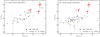 |
Fig. 15. N V and C IV column densities of associated (left panel) and intervening (right panel) absorbers from Fechner & Richter (2009) (in grey and blue: secondary detections for the quasar) and Yggdrasil detections (red). |
We have an additional set of quasar absorbers with which to compare the C IV and Si IV column densities we measured. Quasar absorption for the ionised gas, in particular, has been measured by Songaila (1998) and D’Odorico et al. (2013). In the former, absorption is from the IGM, while the latter results show quasar-associated absorption at much higher redshifts of z > 6. This comparison is shown in Fig. 16. This figure shows that Yggdrasil absorbers agreee better with the associated absorbers of D’Odorico et al. (2013) than with the intervening absorbers of Songaila (1998). These order-of-magnitude comparisons show that the absorbers in the Yggdrasil spectrum are much more likely to be associated with the galaxy halo.
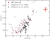 |
Fig. 16. NC IV relative to NSi I for absorbers in the IGM in Songaila (1998) and quasar-associated absorbers in D’Odorico et al. (2013). |
8. Photoionisation modelling
We used a photoionisation modelling code to determine the main ionising mechanisms that produce the observed ionised gas and its column densities in the absorbing gas shells surrounding Yggdrasil. A very detailed study of this has been carried out by Binette et al. (2000), who obtained a metallicity of Z/Z⊙ ≃ 0.02 (Z⊙ being the solar metallicity) for the strongest Lyα absorbers. Their findings also indicated that emitting and absorbing gas are not co-spatial and that the gas is best described by an H I volume density of nH I = 100 cm−3. In addition to this, Binette et al. (2006) sought to determine the ionising mechanism behind the absorbers in this source, and thus showed that stellar photoionisation results in the H I and C IV absorber column densities
It is worth noting that their conclusions were obtained using only column densities for H I and C IV. With our recent detection of N V absorption at the same velocity as the strong Lyα absorber, we can provide more insight to these findings. Given the detection of N V, flux from the metagalactic background may be too weak to ionise the absorbers. At z ≥ 2.7, He II reionisation was more active than it is at lower redshifts, meaning that ionising photons with energies of Eγ > 54.4 eV had megaparsec-scale mean free paths (Shull et al. 2010; McQuinn 2016). The metagalactic background is therefore less likely to be a strong ionising mechanism powering the absorbers in the halo of Yggdrasil.
We also considered the possibility that shocks by the powerful radio jets may ionise the gas. This was proposed by Dopita & Sutherland (1995), and observational evidence for shock ionisation in HzRGs has been shown by several authors, particularly in sources with relatively small radio sources that are still contained within the host galaxy (e.g. Allen et al. 1998; Best et al. 2000; De Breuck et al. 2000). A powerful diagnostic of shock-ionised emission are the line ratios of carbon: in shock ionised regions, we expect the C II] λ2326 line to be as strong as its higher ionisation counterparts. Our MUSE spectrum (Fig. 2) contains three carbon lines and allows us to make this test. Interestingly, the C II] λ1906, 1908 line contains a much stronger blueshifted component than the C III] and C IV λλ1548, 1550 lines. These high C II]/C III] and C II]/C IV ratios are consistent with shock ionisation (see e.g. Fig. 1 of Best et al. 2000). This provides evidence to our claim that this blueshifted gas near the western radio lobe is an outflow driven by the radio jet. On the other hand, the radio of the main component near the AGN has a C III]/C II] ratio of ∼2.4, which places it squarely in the AGN photoionisation region. This main velocity component dominates the flux of all the other emission lines, therefore we did not consider shock ionisation as a relevant contributor in those lines.
Stellar photoionisation is a possibility as well. The star formation rate (SFR) in Yggdrasil, however, is SFR = 41 M⊙ yr−1 (Falkendal et al. 2019) and may be insufficient to produce the starburst activity that would ionise the absorbers. Another possibility is the AGN, which we can expect to produce a strong enough ionising continuum to produce the detected absorption.
We therefore revisited the analysis by running photoionisation models using CLOUDY C17 (Ferland et al. 2017), a spectral synthesis code designed to run grid models that provide simulated chemical abundances in photoionised gas. Within the halo of Yggdrasil, we have shown that Lyα absorbers are at the same velocity as C IV, N V, and Si IV absorbers, suggesting that the gas tracers occupy the same gas volume.
The ionisation parameter is defined as  is the quotient of the volume density of hydrogen-ionising photons and the volume density of hydrogen atoms contained within the gas. Here, r is the line-of-sight distance from the ionising source to the gas, nH I is the hydrogen density, Lν is the specific luminosity, and ν is the observing frequency such that the integral,
  is the luminosity of the ionising source. Provided that we can determine U(r) for the radiation field ionising the absorbing gas, we can also compute the distance of the gas from the radiation source along the line of sight.
8.1. AGN photoionisation of the absorbers
We have shown in the comparison to quasar absorbers in Fechner & Richter (2009) that the absorbers in Yggdrasil are located within the CGM rather than IGM. In the CLOUDY model, we used a power law spectral energy distribution (SED; where the ionising flux is given by Sν ∝ να) to simulate the incident radiation produced by the AGN. In this, we tested α = −1.5 and α = −1.0 to model the photoionisation of the gas by an AGN (e.g. Villar-Martin et al. 1997; Feltre et al. 2016; Humphrey et al. 2019).
The model grid consists of a set of input parameters. The hydrogen density was fixed to nH I = 100 cm−3, which is commonly adopted to describe the low-density diffuse gas that we expect in the extended absorbers (e.g. Binette et al. 2000; Humphrey et al. 2008a). The metallicity (Z) was varied over a range of values between Z/Z⊙ = 0.01 and 10. The H I column density NH I was taken from the line-fitting results (shown in Table 5). The ionisation parameter varied over the range 10−2.5 < U < 10−1 in 0.5 dex increments.
We did not include the effects of dust extinction because the surface brightness of emission re-radiated by dust, detected by the Atacama Large Millimetre/sub-mm Array (ALMA) at an observing frequency of νobs = 235 GHz is lower in Yggdrasil than in the offset region at projected distances of d = 65–80 kpc from the host galaxy, where three resolved dusty companions are observed (G16). This observation implies that dust has a negligible contribution to the SED at the host galaxy. Moreover, Falkendal et al. (2019) have shown that the SFR in Yggdrasil is lower than that which is detected in the companion sources, collectively.
In the CLOUDY models, we have assumed an open or plane-parallel geometry for the absorbing gas medium, which implies that the cloud depth is significantly smaller than its inner radius, or more simply, the distance between the ionising continuum source and the illuminated gas surface. Following the findings from Binette et al. (2000), we assumed that the absorbers are not co-spatial with the emitting gas.
The column density measures we obtain are shown against the simulated column densities in Figs. 17 and 18, and the results indicate that absorbers 1 and 3 may have supersolar metallicities of Z/Z⊙ ≃ 10 and 5, respectively. However, due to uncertainties in line-fitting, the column densities obtained are upper limits and no proper conclusion can be drawn about the metallicities of the absorbers. If these models were to suggest super-solar metallicity in absorbers. this would not be a unusual given that super-solar metallicites in HzRG absorption line gas have been measured before (Jarvis et al. 2003; Binette et al. 2006). Jarvis et al. (2003) showed that absorbers in the halo of the z = 2.23 radio galaxy, 0200+015, had Z/Z⊙ ∼ 10 and covering factors of C < 1.0. This implied that the absorbers are likely to be co-spatial with the EELR. Based on Fig. 19, the measured column densities of absorber 2 prove that its metallicity is closer to a value of Z/Z⊙ = 0.01. The results also suggest that the N V column density is under-predicted by the Z/Z⊙ = 0.01 model. We explore the possible reasons for this in the following section.
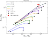 |
Fig. 17. N V and C IV column densities obtained from CLOUDY photoionisation models. The predicted column densities are for absorber 1, which has an H I column density of NH I = 1014.2 cm−2 that is kept constant as U(r) increases from U = 10−2.5 to U = 10−1 in increments of 0.5 dex. The metallicities Z/Z⊙ = 0.1, 0.5, 1, and 5 are tested for spectral indices α = −1.0 (solid lines) and α = −1.5 (dashed lines). |
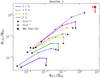 |
Fig. 18. N V and C IV column densities obtained from CLOUDY photoionisation models similar to those in Fig. 17. The models shown here are for absorber 3 because the H I column density is kept constant at NH I = 1013.3 cm−2. The metallicities tested are Z/Z⊙ = 0.1, 0.5, 1, and 5. |
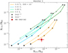 |
Fig. 19. N V and C IV column densities obtained from photoionisation CLOUDY models similar to those in Fig. 17. The models shown here are for absorber 2, the strong absorber, because the H I column density is kept constant at NH I = 1019.2 cm−2. The nitrogen abundance at Z/Z⊙ = 0.01 has also been enhanced by a factor of 10 (orange curve) i.e. N/H = 10. |
8.2. Nitrogen abundances under-predicted by AGN photoionisation
The assumed power laws for the ionising continuum do not re-produce the metal ion column densities observed in the strong absorber (absorber 2). We are certain that the C IV column density is well measured given its agreement to literature values (Jarvis et al. 2003; G16). The N V cannot be compared to any previous results other than the quasar absorbers shown in Fig. 15, but has been fit with a similar level of uncertainty as C IV. The results shown in Fig. 19 indicate that AGN photoionisation alone cannot produce the measured N V column densities. At the same time, a softer ionising continuum is also insufficient in producing a high-ionisation tracer such as N V. In other words, a power law under-predicts the measured N V column density for the strong Lyα absorber. We therefore explored secondary nitrogen production, enhanced nitrogen abundances, and a lower H I column density as possible reasons for under-predicted nitrogen abundances.
8.2.1. Secondary nitrogen production
The under-predicted nitrogen abundance may result from scaling the nitrogen abundance (relative to hydrogen) according to the solar value, that is, N/H ∝ (N/H)⊙. We propose that secondary nitrogen production by intermediate-mass stars with M/M⊙ = 1−8 (e.g. Henry et al. 2000). In this process, abundances scale as N/O ∝ O/H ∝ Z (with N, O, and H being the nitrogen, oxygen, and hydrogen abundances and Z the metallicity of the gas). This implies that N/H ∝ (O/H)2 ∝ Z2. However, secondary nitrogen production is known to occur in gas with super-solar metallicities (i.e. Z/Z⊙ ≥ 1.0) while primary nitrogen production dominates at sub-solar metallicities (e.g. Hamann & Ferland 1993). We can consider secondary nitrogen the cause of nitrogen enhancement in absorber 2. Figure 15a shows that the absorbers in Yggdrasil have similar column densities as associated quasar absorbers in the Fechner & Richter (2009) sample. In this study, secondary nitrogen production is posited as a reason for the nitrogen enrichment of the quasar absorbers.
If secondary nitrogen production from carbon and oxygen in the CNO cycle were to cause the enhanced nitrogen abundance in the strong absorber, the absorber would have a higher metallicity than originally determined (Z/Z⊙ ≃ 0.02; Binette et al. 2000, 2006). As is the case for the EELR in S18, where is said to occur, secondary nitrogen production occurs for a gas metallicity of Z/Z⊙ ≃ 2.0. The CLOUDY model grid indicates that in order for gas to be enriched by secondary nitrogen, it would also have a metallicity of Z/Z⊙ ≥ 1.0. This is improbable given that an increase in the cloud metallicity results in an increase in both the C IV and N V column densities. We therefore exclude secondary nitrogen production as a mechanism for the enhancement of nitrogen abundances.
8.2.2. Degeneracy of b and NH II for the strong absorber
The degeneracies between the H I column density NH I and the Doppler parameter have been described in S18, who found two probable best-fit solutions for the b parameter and NH I in absorber 2. These are NH I/cm−2 = 1019.63 with b = 52 km s−1 and NH I/cm−2 = 1015.20 with b = 153 km s−1. Taking the lower H I column density solution as well as the NC IV and NN V measurements from our results, we ran the CLOUDY model grid using the same AGN photoionisation scheme (described in Sect. 8.1).
This time, applying the low H I column density solution (i.e. NH I/cm−2 = 1015.20) to the grid resulted in the observed column density ratios (i.e. NC IV/NH I and NN V/NH I), suggesting that absorber 2 has a supersolar metallicity, Z/Z⊙ ≃ 5. This result differs greatly from the expected abundances from Binette et al. (2000), that is, Z/Z⊙ ≃ 0.02, which was obtained through photoionisation modelling in MAPPINGS IC (Binette et al. 1985; Ferruit et al. 1997). This result may imply that if the cloud had a lower H I column, its metallicity would need to be higher than Z/Z⊙ ≃ 0.01.
8.2.3. Nitrogen abundance enhancement
For the CLOUDY models to reproduce the observed column densities, we require a nitrogen abundance that is greater than the solar abundance by a factor of 10, as Fig. 19 suggests. We can examine occurrences of enhanced nitrogen abundances in similar sources to attempt to find an answer for this.
The photoionisation models shown in Fig. 10 of Binette et al. (2006) seem to suggest that the N V column density of absorber 2 suggests that it may be ionised by the same mechanism that ionises the Lynx arc nebulae, which is a metal-poor H II galaxy at z ≃ 3.32 that has undergone a recent starburst (Villar-Martín et al. 2004). However, this scenario would require stellar photoionisation rather than an AGN. The presence of N V in the absorber presents a strong case for an AGN rather than stellar photoionisation because it has such a high ionisation energy.
To determine whether the current episode of AGN activity has ionised the absorber, we determined its lifespan. The radio size of Yggdrasil is r ≃ 29 kpc (Pentericci et al. 1999), and its approximate expansion speed is v ≃ 0.05c. The age of the radio source therefore is approximately τjet ≃ 2 Myr. The strong absorber, on the other hand, is roughly r ≃ 60 kpc, and has an outflow rate of 400 km s−1 relative to the galactic nucleus. This translates into an approximate outflow timescale of τabs. ≃ 200 Myr. That the radio source is a factor of 100 younger than the absorber implies that the current duty cycle of the radio jet can be responsible for the ionisation of the absorber, but it did not eject the gas that formed absorber 2.
To explain the chemical abundances, we propose that the absorber has been enriched by an early episode of star formation. Metal-rich gas from the ISM is driven by starbursts and through powerful winds, which dilutes the low-metallicity gas in absorber 2. Evidence of this is seen in local massive ellipticals, which are considered the progeny of HzRGs, where nitrogen abundances are enhanced well above that of carbon, that is, [N/Fe] ∼ 0.8−1 and [C/Fe] ∼ 0.3 (for nitrogen, N, carbon, C, and iron, Fe, abundances) as a result of starburst-driven superwinds (Greene et al. 2013, 2015).
8.3. Distances of absorbers from the ionising source
The distance between the AGN and the absorbing gas can be estimated but is dependent on nH I. Given that we cannot constrain the hydrogen density, we have only the ratio of ionisation parameters to infer the distance ratios of two absorbers, for instance,  . Assuming that our measure of nH I = 100 cm−3 is correct, we can approximate the distance of absorber 2 from the AGN using the integrated infrared luminosity,
  , of the host galaxy computed by Falkendal et al. (2019). According to Fig. 19, the ionisation parameter for absorber 2 is approximately U ≃ 10−2.25. Expressing the ionisation parameter as U(r) = L/nH Ir2 (e.g. Różańska et al. 2014), we obtain a distance of
  kpc between absorber 2 and the AGN.
9. Discussion
9.1. Blueshifted emission: companion galaxy or outflow?
There is sufficient evidence to suggest that the preferred environments of radio galaxies are rich clusters and groups. This is at low redshifts (z ≲ 1), where the most radio-loud sources have a higher likelihood of residing in kiloparsec-scale overdense structures (e.g. Best et al. 2007; Karouzos et al. 2014; Magliocchetti et al. 2018; Kolwa et al. 2019). Radio-loud sources are also prevalent in over-dense environments consisting of dusty starburst galaxies and/or Lyα emitters at z > 1.2 (e.g. Hatch et al. 2011; Wylezalek et al. 2013; Dannerbauer et al. 2014; Saito et al. 2015). Based on these findings, we hypothesise that the blueshifted emission in this source systemic redshift may stem from a proto-galaxy or dwarf satellite.
A well-studied example is a Minkowski’s object, associated with the radio galaxy PKS 0123-016, which has an increased SFR due to the passage of the radio source’s jets (van Breugel et al. 1985). The high-velocity dispersions of the blueshifted emission in Yggdrasil imply a different origin of the gas. Only an AGN would produce the turbulent gas motions that can broaden lines such as He II to line widths of FWHM = 1500 km s−1. Furthermore, dwarf galaxies tend to have outflow velocities of ionised gas of vout ≲ 100 km s−1 (Martin 2005). Such velocities are well below the outflow rates we observe in the blueshifted ionised gas, where the velocities are vout ≳ 400 km s−1.
It is more likely that the gas turbulence is driven by the jets. This is also a known occurrence within the gas haloes of powerful radio galaxies (e.g. Humphrey et al. 2006; Morais et al. 2017; Nesvadba et al. 2017a). The jet-driven outflow scenario is well supported in 4.7 GHz radio observations that indicate from rotation measures that radio emission from the western radio lobe in this source propagates over a shorter path length than radio emission from the eastern lobe (e.g. Carilli et al. 1997).
This configuration implies that the radio axis is also tilted at a non-zero inclination angle with respect to the projected plane, as shown Fig. 20. If the jets were parallel to the plane of the sky, we would observe similar rotation measures at both the east and west radio lobes. The rotation measure at the eastern lobe is higher than that at the western lobe. This jet inclination can also explain that the blueshifted emission is an outflow.
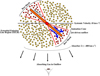 |
Fig. 20. Cross-section schematic of the circumgalactic medium of Yggdrasil based on evidence from the MUSE data and previous measures. The gas has no defined spatial boundaries because its estimates size of d ≳ 60 kpc is merely a minimum. The strong absorber screens emission that originates from the T ≃ 104 − 106 K EELR gas (in yellow), comprising an extended region of ionised gas as well as gas that is directly ionised by the AGN ionisation cone (in red). The absorbing gas (shown as dotted curve) is also metal enriched, as shown by C IV, N V, and Si IV that are detected at the same velocities as the Lyα absorption. The blueshifted component detected in Lyα and He II is a jet-induced outflow (blue arrows). This outflowing, ionised, and turbulent gas is spatially offset from the HSBR of the halo, which implies that the radio jet is tilted relative to the projected plane. The locations of absorber 2 is a line-of-sight projected distance, which is dependent on the ionisation parameter, U(r). |
The kinematics surrounding the jet-gas interactions in the gas halo of Yggdrasil have been measured in previous studies. Villar-Martín et al. (2003) reported that the narrow components of He II emission were blueshifted from the systemic at velocity shifts of Δv ∼ 100 km s−1. This kinematically quiet component identified with an FWHM ∼ 500 km s−1 is shown to extend across the entire halo, well beyond the radio hotspot. This suggests jet-gas interactions. In addition to this, Humphrey et al. (2006) found that the He II gas that has a perturbed component with FWHM = 1760 km s−1 and the quiescent component with FWHM = 750 km s−1, respectively, at a velocity shift of Δv ∼ −250 km s−1 is low-ionisation gas. We find that the blueshifted emission has FWHM = 970 km s−1 at Δv ∼ −1000 km s−1. Although our measured velocity shifts differ slightly from those of previous works, the common thread is that the He II emission is blueshifted relative to systemic and aligned with the radio axis. This indicates jet-gas interactions.
This view agrees well with observations from G16, who reported direct evidence for the ionisation cone to be projected along the radio jet axis in the form of extended He II, C IV, and C III] emission to the south-west of the source. A detailed discussion of the ionised gas kinematics is presented in S18. Their interpretation differs from ours only slightly in that our radio axis is tilted relative to the projected plane.
In addition to He II enhancement, a dust continuum and enhanced SFRs have been observed to the south-west of the inferred centre of the galaxy halo. G16 reported that the strong dust continuum may be a result of starbursts. This is supported by the SFR, which is measured to be 41 M⊙ yr−1 in Yggdrasil compared to 747 M⊙ yr−1 in the dusty regions in the south-west or companion sources (Falkendal et al. 2019). Anti-correlations between radio size and 1.1 mm luminosities (that trace SF) measured from a sample of 16 HzRGs in Humphrey et al. (2011) have explained why more evolved sources, such as Yggdrasil, have experienced a decline in their star formation.
Furthermore, at z > 3.0, metal enrichment and disturbed kinematics of extended gas haloes have been linked to jet-induced star formation in HzRGs (e.g. Reuland et al. 2007). It is not possible to state that there is jet-induced star-formation in this galaxy, however, because the projected radio size of d ≃ 29 kpc shows that the radio emission has not propagated far enough to induce star-formation at d = 65 and 80 kpc from the host galaxy where the companion sources are located (G16).
9.2. Possible origins and the nature of the absorbing gas
We have shown that resonance line scattering or absorption of C IV, N V, and Si IV photons occurs at the same velocities as do the line scattering or absorption of the strong Lyα absorber (absorber 2). Because of the uncertainties in measuring Si IV absorption, we only discuss the main absorber around Lyα, N V, and C IV. We obtained redshifts, column densities, and Doppler parameters for absorbers in the Lyα profile and found that the H I column densities we measured are consistent with previous results (van Ojik et al. 1997; Jarvis et al. 2003; Wilman et al. 2004; G16; S18).
The formation of absorber 2 is well supported by simulations in which the neutral gas column is formed at the bow shock of radio jets and cools to T ∼ 104 − 106 K before fragmenting due to Rayleigh–Taylor (RT) instabilities that are brought about by the radio cocoon (Krause 2002, 2005). S18 also showed that absorber 2 may be outflowing, which is in agreement with this framework. In addition to the high column density absorber, we also observed three H I absorbers with column densities of NH I = 1013−1014 cm−2. The weak absorbers (absorbers 1, 3, and 4) could be fragmented shells of gas that have been disrupted by RT instabilities, hence their low column densities. In this scenario, the absorbers are formed through the ageing of the radio source (Wilman et al. 2004; Binette et al. 2006).
Absorber 2 has a much higher H I column density of NH I/cm−2 = 1019.2. It may be a metal-poor gas shell that was expelled from the galaxy by an early AGN-related feedback event (Jarvis et al. 2003; Binette et al. 2006). We agree with this interpretation given both the strength of the absorber and the sum of its ionised and neutral mass, MT/M⊙ ≥ 5.7 × 10⁹, which is an order of magnitude lower than the stellar mass component of M*/M⊙ = 1.2 × 10¹¹ of the galaxy, implying that a very energetic event would have to be responsible for expelling such a vast amount of gas.
The nitrogen abundance of absorber 2, if photoionised primarily by the AGN, is in excess by a factor of 10 compared to its solar abundance. Because absorber 2 has a low metallicity overall, it may be nitrogen enhanced as a result of stellar winds. Chemically enriched gas from the ISM may have been swept up by stellar winds and progressively diluted the outflowing gas shell.
This scenario is similar to that of the z = 3.09 star-forming galaxy of Wilman et al. (2005), which also contains an emission line region that is covered by a neutral gas shell of H I column density, NH I/cm2 ≃ 1019. The main difference between this source and ours is the SFR, which is much higher in the star-forming galaxy. If the mechanism by which the strong absorber in Yggdrasil has been enriched is a starburst-driven super-wind, it could mean that this process occurred at an earlier epoch, and we now observe the galaxy after a major starburst period has ceased.
10. Summary
We have examined the absorbing gas surrounding the host galaxy of MRC 0943−242, Yggdrasil, using MUSE data. Our results prove that the H I absorbers measured from the Lyα line are at the same velocities as the C IV and N V absorbers. The new integral field unit (IFU) dataset shows that the high H I column density absorbing gas (Lyα absorber 2) with NH I/cm−2 = 1019.2 is a non-isotropic gas medium extending outwards from r ≳ 60 kpc. It has a hydrogen fraction of XH I ≳ 0.8, which makes it a predominantly ionised cloud with a total estimated mass of the neutral and ionised gas of M/M⊙ ≥ 5.7 × 10⁹. Detections of Si II absorption at the same velocity of this absorber suggest that it is ionisation bounded.
Similar to previous studies, we observe a diffuse extension of He II gas in alignment with the VLA-detected radio axis and the HST -detected optical/UV broad-band emission. The ionised gas is interpreted as a jet-induced outflow. The combination of radio axis and the observed He II emission in this IFU data indicates that the radio jet is tilted at a non-zero inclination angle. This finding is well supported by rotation measures in the eastern and western radio lobes of the galaxy, which indicate that the emission from the eastern radio lobe has travelled farther along the line of sight than that emitted from the western lobe.
We also estimated the locations of the absorbers within the halo, assuming that they are outflowing. It is likely that absorber 2 is located at a greater distance from the AGN than absorber 1. Furthermore, the measured absorber column densities in Yggdrasil are similar in magnitude to those of absorbers at velocity shifts of |Δv| < 5000 km s−1 from quasars.
Photoionisation models of the absorbing gas in CLOUDY have shown that ionising radiation from the AGN (for which we assumed a spectral energy distribution with a power-law shape of α = −1) is capable of producing the C IV and N V column densities observed in absorber 2 when the gas has a metallicity of Z/Z⊙ = 0.01 in which the nitrogen abundance is enhanced by a factor of 10 relative to the solar abundance (i.e. N/H = 10). This high column density absorber is interpreted as primordial gas that was propelled outwards by an earlier feedback event (possibly an AGN). The gas has subsequently been ionised by an episode of AGN activity and chemical enriched through stellar winds.
In conclusion, we showed the potential use of wide-field IFU instruments in understanding the configuration of complex systems such as the haloes of HzRGs. Similar future analyses will be fundamental in unveiling the different gas structures surrounding HzRGs, ultimately adding important constraints on the physics of these objects.
Acknowledgments
SK acknowledges the International Max Planck Research Schools (IMPRS) and the European Southern Observatory (ESO). All authors acknowledge the ESO Paranal Observatory as the source for VLT/MUSE data that formed the basis of this work. SK, CDB and JV thank Richard Wilman and Matt J. Jarvis for the ancillary UVES spectrum. We thank Paola Caselli and Ian Smail for providing helpful guidance and suggestions. SK thanks Marios Chatzikos and Fran Guzmán for support with CLOUDY. This study has made use of data from the European Space Agency (ESA) mission Gaia (https://www.cosmos.esa.int/gaia), processed by the Gaia Data Processing and Analysis Consortium (DPAC, https://www.cosmos.esa.int/web/gaia/dpac/consortium). Funding for the DPAC has been provided by national institutions, in particular the institutions participating in the Gaia Multilateral Agreement. This work is on observations collected at the European Southern Observatory under ESO programmes 096.B-0752(A) and 068.B-0086(A). It is also based on observations made with the NASA/ESA Hubble Space Telescope, and obtained from the Hubble Legacy Archive, which is a collaboration between the Space Telescope Science Institute (STScI/NASA), the Space Telescope European Coordinating Facility (ST-ECF/ESA) and the Canadian Astronomy Data Centre (CADC/NRC/CSA). MVM acknowledges support from the Spanish Ministerio de Ciencia, Innovación y Universidades (former Ministerio de Economía y Competitividad) through the grant AYA2015-64346-C2-2-P. AH acknowledges FCT Fellowship SFRH/BPD/107919/2015; Support from European Community Programme (FP7/2007-2013) under grant agreement No. PIRSES-GA-2013-612701 (SELGIFS); Support from FCT through national funds (PTDC/FIS-AST/3214/2012 and UID/FIS/04434/2013), and by FEDER through COMPETE (FCOMP-01-0124-FEDER-029170) and COMPETE2020 (POCI-01-0145-FEDER-007672). AH acknowledges support from the FCT-CAPES Transnational Cooperation Project “Parceria Estratégica em Astrofísica Portugal-Brasil”.
References
- Allen, M. G., Dopita, M. A., & Tsvetanov, Z. I. 1998, ApJ, 493, 571 [NASA ADS] [CrossRef] [Google Scholar]
- Arrigoni Battaia, F., Prochaska, J. X., Hennawi, J. F., et al. 2018, MNRAS, 473, 3907 [NASA ADS] [CrossRef] [Google Scholar]
- Bacon, R., Vernet, J., Borisova, E., et al. 2014, The Messenger, 157, 13 [NASA ADS] [Google Scholar]
- Barkana, R., & Loeb, A. 2003, Nature, 421, 341 [NASA ADS] [CrossRef] [Google Scholar]
- Barnes, L. A., Garel, T., & Kacprzak, G. G. 2014, PASP, 126, 969 [NASA ADS] [CrossRef] [Google Scholar]
- Baum, S. A., Heckman, T. M., Bridle, A., van Breugel, W. J. M., & Miley, G. K. 1988, ApJS, 68, 643 [NASA ADS] [CrossRef] [Google Scholar]
- Bechtold, J. 2001, ArXiv e-prints [arXiv:astro-ph/0112521] [Google Scholar]
- Best, P. N., Röttgering, H. J. A., & Longair, M. S. 2000, MNRAS, 311, 23 [NASA ADS] [CrossRef] [Google Scholar]
- Best, P. N., von der Linden, A., Kauffmann, G., Heckman, T. M., & Kaiser, C. R. 2007, MNRAS, 379, 894 [NASA ADS] [CrossRef] [Google Scholar]
- Binette, L., Dopita, M. A., & Tuohy, I. R. 1985, ApJ, 297, 476 [NASA ADS] [CrossRef] [Google Scholar]
- Binette, L., Wilson, A. S., & Storchi-Bergmann, T. 1996, A&A, 312, 365 [NASA ADS] [Google Scholar]
- Binette, L., Kurk, J. D., Villar-Martín, M., & Röttgering, H. J. A. 2000, A&A, 356, 23 [NASA ADS] [Google Scholar]
- Binette, L., Groves, B., Villar-Martín, M., Fosbury, R. A. E., & Axon, D. J. 2003, A&A, 405, 975 [NASA ADS] [CrossRef] [EDP Sciences] [Google Scholar]
- Binette, L., Wilman, R. J., Villar-Martín, M., et al. 2006, A&A, 459, 31 [NASA ADS] [CrossRef] [EDP Sciences] [Google Scholar]
- Bischetti, M., Piconcelli, E., Vietri, G., et al. 2017, A&A, 598, A122 [NASA ADS] [CrossRef] [EDP Sciences] [Google Scholar]
- Carilli, C. L., Röttgering, H. J. A., van Ojik, R., Miley, G. K., & van Breugel, W. J. M. 1997, ApJS, 109, 1 [NASA ADS] [CrossRef] [Google Scholar]
- Cashman, F. H., Kulkarni, V. P., Kisielius, R., Ferland, G. J., & Bogdanovich, P. 2017, ApJS, 230, 8 [NASA ADS] [CrossRef] [Google Scholar]
- Churchill, C. 1995, Introduction to Echelle Data Reduction using IRAF, Lick Observatory Technical Report No. 74 (Astrophysics and Space Science Library) [Google Scholar]
- Cicone, C., Maiolino, R., Sturm, E., et al. 2014, A&A, 562, A21 [NASA ADS] [CrossRef] [EDP Sciences] [Google Scholar]
- Dannerbauer, H., Kurk, J. D., De Breuck, C., et al. 2014, A&A, 570, A55 [NASA ADS] [CrossRef] [EDP Sciences] [Google Scholar]
- De Breuck, C., van Breugel, W., Minniti, D., et al. 1999, A&A, 352, L51 [NASA ADS] [Google Scholar]
- De Breuck, C., Röttgering, H., Miley, G., van Breugel, W., & Best, P. 2000, A&A, 362, 519 [NASA ADS] [Google Scholar]
- De Breuck, C., van Breugel, W., Stanford, S. A., et al. 2002, AJ, 123, 637 [NASA ADS] [CrossRef] [Google Scholar]
- De Breuck, C., Neri, R., Morganti, R., et al. 2003, A&A, 401, 911 [NASA ADS] [CrossRef] [EDP Sciences] [Google Scholar]
- Dekker, H., D’Odorico, S., Kaufer, A., Delabre, B., & Kotzlowski, H. 2000, in Optical and IR Telescope Instrumentation and Detectors, eds. M. Iye, & A. F. Moorwood, SPIE Conf. Ser., 4008, 534 [Google Scholar]
- D’Odorico, S., Cristiani, S., Dekker, H., et al. 2000, in Discoveries and Research Prospects from 8- to 10-Meter-Class Telescopes, ed. J. Bergeron, et al., SPIE Conf. Ser., 4005, 121 [NASA ADS] [CrossRef] [Google Scholar]
- D’Odorico, V., Cupani, G., Cristiani, S., et al. 2013, MNRAS, 435, 1198 [NASA ADS] [CrossRef] [Google Scholar]
- Dopita, M. A., & Sutherland, R. S. 1995, ApJ, 455, 468 [NASA ADS] [CrossRef] [Google Scholar]
- Emonts, B. H. C., De Breuck, C., Lehnert, M. D., et al. 2015, A&A, 584, A99 [NASA ADS] [CrossRef] [EDP Sciences] [Google Scholar]
- Emonts, B. H. C., Lehnert, M. D., Dannerbauer, H., et al. 2018, MNRAS, 477, L60 [NASA ADS] [CrossRef] [Google Scholar]
- Falkendal, T., De Breuck, C., Lehnert, M. D., et al. 2019, A&A, 621, A27 [NASA ADS] [CrossRef] [EDP Sciences] [Google Scholar]
- Fechner, C., & Richter, P. 2009, A&A, 496, 31 [NASA ADS] [CrossRef] [EDP Sciences] [Google Scholar]
- Feltre, A., Charlot, S., & Gutkin, J. 2016, MNRAS, 456, 3354 [Google Scholar]
- Ferland, G. J., Chatzikos, M., Guzmán, F., et al. 2017, Rev. Mex. Astron. Astrofis., 53, 385 [NASA ADS] [Google Scholar]
- Ferruit, P., Binette, L., Sutherland, R. S., & Pecontal, E. 1997, A&A, 322, 73 [NASA ADS] [Google Scholar]
- Gaia Collaboration (Prusti, T., et al.) 2016, A&A, 595, A1 [NASA ADS] [CrossRef] [EDP Sciences] [Google Scholar]
- Gaia Collaboration (Brown, A. G. A., et al.) 2018, A&A, 616, A1 [NASA ADS] [CrossRef] [EDP Sciences] [Google Scholar]
- Greene, J. E., Murphy, J. D., Graves, G. J., et al. 2013, ApJ, 776, 64 [NASA ADS] [CrossRef] [Google Scholar]
- Greene, J. E., Janish, R., Ma, C.-P., et al. 2015, ApJ, 807, 11 [NASA ADS] [CrossRef] [Google Scholar]
- Gullberg, B., De Breuck, C., Lehnert, M. D., et al. 2016, A&A, 586, A124 [NASA ADS] [CrossRef] [EDP Sciences] [Google Scholar]
- Hamann, F., & Ferland, G. 1993, ApJ, 418, 11 [NASA ADS] [CrossRef] [Google Scholar]
- Hatch, N. A., De Breuck, C., Galametz, A., et al. 2011, MNRAS, 410, 1537 [NASA ADS] [Google Scholar]
- Heckman, T. M., Lehnert, M. D., van Breugel, W., & Miley, G. K. 1991, ApJ, 370, 78 [NASA ADS] [CrossRef] [Google Scholar]
- Henry, R. B. C., Edmunds, M. G., & Köppen, J. 2000, ApJ, 541, 660 [NASA ADS] [CrossRef] [Google Scholar]
- Hernández-García, L., Vietri, G., Panessa, F., et al. 2018, MNRAS, 478, 4634 [NASA ADS] [CrossRef] [Google Scholar]
- Holt, J., Tadhunter, C. N., & Morganti, R. 2008, MNRAS, 387, 639 [NASA ADS] [CrossRef] [Google Scholar]
- Humphrey, A., Villar-Martín, M., Fosbury, R., Vernet, J., & di Serego Alighieri, S. 2006, MNRAS, 369, 1103 [NASA ADS] [CrossRef] [Google Scholar]
- Humphrey, A., Villar-Martín, M., Fosbury, R., et al. 2007, MNRAS, 375, 705 [NASA ADS] [CrossRef] [Google Scholar]
- Humphrey, A., Villar-Martín, M., Vernet, J., et al. 2008a, MNRAS, 383, 11 [NASA ADS] [CrossRef] [Google Scholar]
- Humphrey, A., Villar-Martín, M., Sánchez, S. F., et al. 2008b, MNRAS, 390, 1505 [NASA ADS] [Google Scholar]
- Humphrey, A., Zeballos, M., Aretxaga, I., et al. 2011, MNRAS, 418, 74 [NASA ADS] [CrossRef] [Google Scholar]
- Humphrey, A., Vernet, J., Villar-Martín, M., et al. 2013, ApJ, 768, L3 [NASA ADS] [CrossRef] [Google Scholar]
- Humphrey, A., Villar-Martín, M., Binette, L., & Raj, R. 2019, A&A, 621, A10 [NASA ADS] [CrossRef] [EDP Sciences] [Google Scholar]
- Jarvis, M. J., Rawlings, S., Eales, S., et al. 2001, MNRAS, 326, 1585 [NASA ADS] [CrossRef] [Google Scholar]
- Jarvis, M. J., Wilman, R. J., Röttgering, H. J. A., & Binette, L. 2003, MNRAS, 338, 263 [NASA ADS] [CrossRef] [Google Scholar]
- Karouzos, M., Jarvis, M. J., & Bonfield, D. 2014, MNRAS, 439, 861 [NASA ADS] [CrossRef] [Google Scholar]
- Keenan, F. P., Ahmed, S., Brage, T., et al. 2002, MNRAS, 337, 901 [NASA ADS] [CrossRef] [Google Scholar]
- Kolwa, S., Jarvis, M. J., McAlpine, K., & Heywood, I. 2019, MNRAS, 482, 5156 [NASA ADS] [CrossRef] [Google Scholar]
- Krause, M. 2002, A&A, 386, L1 [NASA ADS] [CrossRef] [EDP Sciences] [Google Scholar]
- Krause, M. 2005, A&A, 436, 845 [NASA ADS] [CrossRef] [EDP Sciences] [Google Scholar]
- Krogager, J. K. 2018, ArXiv e-prints [arXiv:1803.01187] [Google Scholar]
- Magliocchetti, M., Popesso, P., Brusa, M., & Salvato, M. 2018, MNRAS, 478, 3848 [NASA ADS] [CrossRef] [Google Scholar]
- Martin, C. L. 2005, ApJ, 621, 227 [Google Scholar]
- McCarthy, P. J., Spinrad, H., van Breugel, W., et al. 1990a, ApJ, 365, 487 [NASA ADS] [CrossRef] [Google Scholar]
- McCarthy, P. J., Kapahi, V. K., van Breugel, W., & Subrahmanya, C. R. 1990b, AJ, 100, 1014 [NASA ADS] [CrossRef] [Google Scholar]
- McCarthy, P. J., Baum, S. A., & Spinrad, H. 1996, ApJS, 106, 281 [NASA ADS] [CrossRef] [Google Scholar]
- McQuinn, M. 2016, ARA&A, 54, 313 [NASA ADS] [CrossRef] [Google Scholar]
- Morais, S. G., Humphrey, A., Villar-Martín, M., et al. 2017, MNRAS, 465, 2698 [NASA ADS] [CrossRef] [Google Scholar]
- Mullaney, J. R., Alexander, D. M., Fine, S., et al. 2013, MNRAS, 433, 622 [NASA ADS] [CrossRef] [Google Scholar]
- Nesvadba, N. P. H., Lehnert, M. D., Eisenhauer, F., et al. 2006, ApJ, 650, 693 [NASA ADS] [CrossRef] [Google Scholar]
- Nesvadba, N. P. H., Lehnert, M. D., De Breuck, C., Gilbert, A. M., & van Breugel, W. 2008, A&A, 491, 407 [NASA ADS] [CrossRef] [EDP Sciences] [Google Scholar]
- Nesvadba, N. P. H., De Breuck, C., Lehnert, M. D., Best, P. N., & Collet, C. 2017a, A&A, 599, A123 [NASA ADS] [CrossRef] [EDP Sciences] [Google Scholar]
- Nesvadba, N. P. H., Drouart, G., De Breuck, C., et al. 2017b, A&A, 600, A121 [NASA ADS] [CrossRef] [EDP Sciences] [Google Scholar]
- Newville, M., Stensitzki, T., Allen, D. B., et al. 2016, Astrophysics Source Code Library [record ascl:1606.014] [Google Scholar]
- Oppenheimer, B. D., & Davé, R. 2008, MNRAS, 387, 577 [NASA ADS] [CrossRef] [Google Scholar]
- Oppenheimer, B. D., Davé, R., Kereš, D., et al. 2010, MNRAS, 406, 2325 [NASA ADS] [CrossRef] [Google Scholar]
- Oppenheimer, B. D., Schaye, J., Crain, R. A., Werk, J. K., & Richings, A. J. 2018, MNRAS, 481, 835 [NASA ADS] [CrossRef] [Google Scholar]
- Pentericci, L., Röttgering, H. J. A., Miley, G. K., et al. 1999, A&A, 341, 329 [NASA ADS] [Google Scholar]
- Perna, M., Cresci, G., Brusa, M., et al. 2019, A&A, 623, A171 [NASA ADS] [CrossRef] [EDP Sciences] [Google Scholar]
- Péroux, C., Petitjean, P., Aracil, B., Irwin, M., & McMahon, R. G. 2004, A&A, 417, 443 [NASA ADS] [CrossRef] [EDP Sciences] [Google Scholar]
- Planck Collaboration XIII. 2016, A&A, 594, A13 [NASA ADS] [CrossRef] [EDP Sciences] [Google Scholar]
- Rakshit, S., & Woo, J.-H. 2018, ApJ, 865, 5 [NASA ADS] [CrossRef] [Google Scholar]
- Reuland, M., van Breugel, W., Röttgering, H., et al. 2003, ApJ, 592, 755 [NASA ADS] [CrossRef] [Google Scholar]
- Reuland, M., van Breugel, W., de Vries, W., et al. 2007, AJ, 133, 2607 [NASA ADS] [CrossRef] [Google Scholar]
- Rocca-Volmerange, B., Le Borgne, D., De Breuck, C., Fioc, M., & Moy, E. 2004, A&A, 415, 931 [NASA ADS] [CrossRef] [EDP Sciences] [Google Scholar]
- Rottgering, H. J. A., Hunstead, R. W., Miley, G. K., van Ojik, R., & Wieringa, M. H. 1995, MNRAS, 277, 389 [NASA ADS] [CrossRef] [Google Scholar]
- Rottgering, H. J. A., van Ojik, R., Miley, G. K., et al. 1997, A&A, 326, 505 [NASA ADS] [Google Scholar]
- Różańska, A., Nikołajuk, M., Czerny, B., et al. 2014, New Astron., 28, 70 [NASA ADS] [CrossRef] [Google Scholar]
- Saito, T., Matsuda, Y., Lacey, C. G., et al. 2015, MNRAS, 447, 3069 [NASA ADS] [CrossRef] [Google Scholar]
- Seymour, N., Stern, D., De Breuck, C., et al. 2007, ApJS, 171, 353 [NASA ADS] [CrossRef] [Google Scholar]
- Shull, J. M., France, K., Danforth, C. W., Smith, B., & Tumlinson, J. 2010, ApJ, 722, 1312 [NASA ADS] [CrossRef] [Google Scholar]
- Silva, M., Humphrey, A., Lagos, P., et al. 2018a, MNRAS, 481, 1401 [NASA ADS] [CrossRef] [Google Scholar]
- Silva, M., Humphrey, A., Lagos, P., et al. 2018b, MNRAS, 474, 3649 [NASA ADS] [CrossRef] [Google Scholar]
- Songaila, A. 1998, AJ, 115, 2184 [NASA ADS] [CrossRef] [Google Scholar]
- Soto, K. T., Lilly, S. J., Bacon, R., Richard, J., & Conseil, S. 2016, MNRAS, 458, 3210 [NASA ADS] [CrossRef] [Google Scholar]
- Swinbank, A. M., Vernet, J. D. R., Smail, I., et al. 2015, MNRAS, 449, 1298 [NASA ADS] [CrossRef] [Google Scholar]
- Tadhunter, C. N., Fosbury, R. A. E., & Quinn, P. J. 1989, MNRAS, 240, 225 [NASA ADS] [CrossRef] [Google Scholar]
- Tepper-García, T. 2006, MNRAS, 369, 2025 [NASA ADS] [CrossRef] [Google Scholar]
- Tumlinson, J., Peeples, M. S., & Werk, J. K. 2017, ARA&A, 55, 389 [NASA ADS] [CrossRef] [Google Scholar]
- van Breugel, W., Filippenko, A. V., Heckman, T., & Miley, G. 1985, ApJ, 293, 83 [NASA ADS] [CrossRef] [Google Scholar]
- van Breugel, W., de Vries, W., Croft, S., et al. 2006, Astron. Nachr., 327, 175 [NASA ADS] [CrossRef] [Google Scholar]
- van Ojik, R., Roettgering, H. J. A., Carilli, C. L., et al. 1996, A&A, 313, 25 [NASA ADS] [Google Scholar]
- van Ojik, R., Roettgering, H. J. A., Miley, G. K., & Hunstead, R. W. 1997, A&A, 317, 358 [NASA ADS] [Google Scholar]
- Vernet, J., Fosbury, R. A. E., Villar-Martín, M., et al. 2001, A&A, 366, 7 [NASA ADS] [CrossRef] [EDP Sciences] [Google Scholar]
- Vernet, J., Lehnert, M. D., De Breuck, C., et al. 2017, A&A, 602, L6 [NASA ADS] [CrossRef] [EDP Sciences] [Google Scholar]
- Villar-Martin, M., Tadhunter, C., & Clark, N. 1997, A&A, 323, 21 [NASA ADS] [Google Scholar]
- Villar-Martín, M., Binette, L., & Fosbury, R. A. E. 1999a, A&A, 346, 7 [NASA ADS] [Google Scholar]
- Villar-Martín, M., Fosbury, R. A. E., Binette, L., Tadhunter, C. N., & Rocca-Volmerange, B. 1999b, A&A, 351, 47 [NASA ADS] [Google Scholar]
- Villar-Martín, M., Vernet, J., di Serego Alighieri, S., et al. 2003, MNRAS, 346, 273 [NASA ADS] [CrossRef] [Google Scholar]
- Villar-Martín, M., Cerviño, M., & González Delgado, R. M. 2004, MNRAS, 355, 1132 [NASA ADS] [CrossRef] [Google Scholar]
- Villar-Martín, M., Humphrey, A., De Breuck, C., et al. 2007, MNRAS, 375, 1299 [NASA ADS] [CrossRef] [Google Scholar]
- Weilbacher, P. M., Streicher, O., Urrutia, T., et al. 2014, Astron. Data Anal. Softw. Syst. XXIII, 485, 451 [Google Scholar]
- Wilman, R. J., Jarvis, M. J., Röttgering, H. J. A., & Binette, L. 2004, MNRAS, 351, 1109 [NASA ADS] [CrossRef] [Google Scholar]
- Wilman, R. J., Gerssen, J., Bower, R. G., et al. 2005, Nature, 436, 227 [NASA ADS] [CrossRef] [Google Scholar]
- Wilson, A. S., Binette, L., & Storchi-Bergmann, T. 1997, ApJ, 482, L131 [NASA ADS] [CrossRef] [Google Scholar]
- Wylezalek, D., Galametz, A., Stern, D., et al. 2013, ApJ, 769, 79 [NASA ADS] [CrossRef] [Google Scholar]
- Zirm, A. W., Overzier, R. A., Miley, G. K., et al. 2005, ApJ, 630, 68 [NASA ADS] [CrossRef] [Google Scholar]
All Tables
Lower and upper bounds placed on initial conditions in the line-fitting routine.
Doublet constraints, set by atomic physics, are embedded in the fitting to obtain best-fit results for C IV, N V, and Si IV+O IV].
Best-fit results to the absorbers in the UVES Lyα spectrum from this work and from Jarvis et al. (2003) and Wilman et al. (2004).
Best-fit results to the non-absorbed emission in the UVES spectrum. The flux units are arbitrary (arb.).
All Figures
|
Fig. 1. MUSE line and continuum (white-light) image of MRC 0943−242. At the centre of the image is the high surface brightness region of the galaxy halo. The sub-cube aperture from which the spectrum in Fig. 2 is obtained is shown within the circle. The UVES slit (dotted outline) has a 1.2″ width and extends over 5″. |
| In the text | |
|
Fig. 2. MUSE spectrum of the high surface brightness region in the halo of MRC 0943−243. The spectrum contains several rest-frame UV lines that are labelled and indicated by the dashed vertical lines. The upper panel shows the entire flux density range for the spectrum, while the lower panel covers only the low flux density range to show the lower S/N lines more clearly. |
| In the text | |
|
Fig. 3. He II λ1640 line in the MUSE spectrum (shown in Fig. 2). The line profile has been continuum subtracted. The best-fit model (red) consists of two Gaussian profiles. The first Gaussian component (in blue) models the excess blue wing emission at the negative velocities, while the second component (in orange) models the emission at the systemic velocity of the galaxy. |
| In the text | |
|
Fig. 4. MUSE-detected continuum-subtracted Lyα (upper panel) and ancillary UVES-detected Lyα (lower panel) for Yggdrasil. The best-fit line model (red) combines Lyα emission consisting of blueshifted and systemic components, as well as the four known absorption troughs. |
| In the text | |
|
Fig. 5. Best-fit line model fit to C IV λλ1548, 1551 detected with MUSE. The green and orange dashed lines represent the underlying doublet emission at wavelengths of 1548 Å and 1551 Å, which are the rest-frame velocities, in the upper and lower axes, respectively. Three Voigt profiles model the absorbers for each emission line in the doublet. |
| In the text | |
|
Fig. 6. Best-fit line model to N V λλ1238, 1242 detected with MUSE. The green and orange dashed lines represent the underlying doublet emission at the rest-frame wavelengths 1238 Å and 1242 Å, which are fixed to the systemic velocity in the upper and lower axes, respectively. Three Voigt profiles model the absorbers for each emission line in the doublet. |
| In the text | |
|
Fig. 7. Best fit line model to the intercombination Si IV λλ1393, 1402 + O IV] line detected with MUSE. The green and orange dashed lines represent the underlying doublet emission at the rest-frame wavelengths, 1393 Å and 1402 Å, which are fixed to the systemic velocity in the upper and low axes, respectively. The O IV] quintuplet line emission is shown in purple. |
| In the text | |
|
Fig. 8. Si II λ1260 absorption line fit with a single Gaussian component. The best-fit line is shown in red. |
| In the text | |
|
Fig. 9. Si II λ1527 absorption line fit with a single Gaussian component. The best-fit line is shown in red. |
| In the text | |
|
Fig. 10. Relative velocities of Lyα, N V, and C IV and Si II absorbers from this work as well as those from G16 and S18. The vertical dash-dotted (black) line indicates the systemic velocity and its error (shaded grey). The horizontal dotted lines (grey) distinguish between the different absorbers. |
| In the text | |
|
Fig. 11. C III] λλ1906, 1908 doublet line-fit consisting of a blueshifted emission component. |
| In the text | |
|
Fig. 12. C II] λ2326 singlet line-fit consisting of a blueshifted emission component. |
| In the text | |
|
Fig. 13. Broad-band image of the rest-frame UV continuum of MRC 0942−242 from the HST WFPC2 702W (5800−8600 Å) filter. MUSE contours (blue) are overlaid and represent narrow-band emission summed over 6400−6425 Å. The contours are shown at the surface brightness levels, (1.0, 1.6, 2.2, 2.8, 3.4, 4.0) ×10−17 erg s−1 cm−2 arcsec−2. VLA 4.7 GHz radio surface brightness is shown by the red contour levels. The inset 1D spectra show the HSBR (left panel) and offset (right panel) He II emission. The line profiles are extracted from apertures of radius R = 0.6″, shown in green for the HSBR and in cyan for the offset region. The aperture centroids for each are shown in matching colours. The blueshifted and systemic He II emissions are shown in blue and orange, respectively, and the sum of both components is shown in red. |
| In the text | |
|
Fig. 14. MUSE continuum-subtracted narrow-band images showing the spatial variation in He II emission at different wavelength bands. The green and cyan crosses show the centres of the HSBR and offset He II emission from which the line profiles in Fig. 13 are extracted. The 4.7 GHz VLA radio contours are shown in red at the levels 3σ, |
| In the text | |
|
Fig. 15. N V and C IV column densities of associated (left panel) and intervening (right panel) absorbers from Fechner & Richter (2009) (in grey and blue: secondary detections for the quasar) and Yggdrasil detections (red). |
| In the text | |
|
Fig. 16. NC IV relative to NSi I for absorbers in the IGM in Songaila (1998) and quasar-associated absorbers in D’Odorico et al. (2013). |
| In the text | |
|
Fig. 17. N V and C IV column densities obtained from CLOUDY photoionisation models. The predicted column densities are for absorber 1, which has an H I column density of NH I = 1014.2 cm−2 that is kept constant as U(r) increases from U = 10−2.5 to U = 10−1 in increments of 0.5 dex. The metallicities Z/Z⊙ = 0.1, 0.5, 1, and 5 are tested for spectral indices α = −1.0 (solid lines) and α = −1.5 (dashed lines). |
| In the text | |
|
Fig. 18. N V and C IV column densities obtained from CLOUDY photoionisation models similar to those in Fig. 17. The models shown here are for absorber 3 because the H I column density is kept constant at NH I = 1013.3 cm−2. The metallicities tested are Z/Z⊙ = 0.1, 0.5, 1, and 5. |
| In the text | |
|
Fig. 19. N V and C IV column densities obtained from photoionisation CLOUDY models similar to those in Fig. 17. The models shown here are for absorber 2, the strong absorber, because the H I column density is kept constant at NH I = 1019.2 cm−2. The nitrogen abundance at Z/Z⊙ = 0.01 has also been enhanced by a factor of 10 (orange curve) i.e. N/H = 10. |
| In the text | |
|
Fig. 20. Cross-section schematic of the circumgalactic medium of Yggdrasil based on evidence from the MUSE data and previous measures. The gas has no defined spatial boundaries because its estimates size of d ≳ 60 kpc is merely a minimum. The strong absorber screens emission that originates from the T ≃ 104 − 106 K EELR gas (in yellow), comprising an extended region of ionised gas as well as gas that is directly ionised by the AGN ionisation cone (in red). The absorbing gas (shown as dotted curve) is also metal enriched, as shown by C IV, N V, and Si IV that are detected at the same velocities as the Lyα absorption. The blueshifted component detected in Lyα and He II is a jet-induced outflow (blue arrows). This outflowing, ionised, and turbulent gas is spatially offset from the HSBR of the halo, which implies that the radio jet is tilted relative to the projected plane. The locations of absorber 2 is a line-of-sight projected distance, which is dependent on the ionisation parameter, U(r). |
| In the text | |
Current usage metrics show cumulative count of Article Views (full-text article views including HTML views, PDF and ePub downloads, according to the available data) and Abstracts Views on Vision4Press platform.
Data correspond to usage on the plateform after 2015. The current usage metrics is available 48-96 hours after online publication and is updated daily on week days.
Initial download of the metrics may take a while.