| Issue |
A&A
Volume 624, April 2019
|
|
|---|---|---|
| Article Number | A18 | |
| Number of page(s) | 17 | |
| Section | Planets and planetary systems | |
| DOI | https://doi.org/10.1051/0004-6361/201834423 | |
| Published online | 02 April 2019 | |
Precise radial velocities of giant stars
XI. Two brown dwarfs in 6:1 mean motion resonance around the K giant star ν Ophiuchi★,★★
1
Landessternwarte, Zentrum für Astronomie der Universität Heidelberg,
Königstuhl 12,
69117 Heidelberg, Germany
e-mail: This email address is being protected from spambots. You need JavaScript enabled to view it.
2
Department of Earth Sciences, The University of Hong Kong,
Pokfulam Road, Hong Kong
3
Max-Planck-Institut für Astronomie,
Königstuhl 17,
69117 Heidelberg, Germany
4
Department of Physics, The University of Hong Kong,
Pokfulam Road, Hong Kong
Received:
13
October
2018
Accepted:
9
January
2019
Abstract
We present radial-velocity (RV) measurements for the K giant ν Oph (= HIP 88048, HD 163917, HR 6698), which reveal two brown dwarf companions with a period ratio close to 6:1. For our orbital analysis we use 150 precise RV measurements taken at the Lick Observatory between 2000 and 2011, and we combine them with RV data for this star available in the literature. Using a stellar mass of M = 2.7M⊙ for ν Oph and applying a self-consistent N-body model we estimate the minimum dynamical companion masses to be m1 sin i ≈ 22.2 MJup and m2 sin i ≈ 24.7 MJup, with orbital periods P1 ≈ 530 d and P2 ≈ 3185 d. We study a large set of potential orbital configurations for this system, employing a bootstrap analysis and a systematic χν2 grid-search coupled with our dynamical fitting model, and we examine their long-term stability. We find that the system is indeed locked in a 6:1 mean motion resonance (MMR), with Δω and all six resonance angles θ1–θ6 librating around 0°. We also test a large set of coplanar inclined configurations, and we find that the system will remain in a stable resonance for most of these configurations. The ν Oph system is important for probing planetary formation and evolution scenarios. It seems very likely that the two brown dwarf companions of ν Oph formed like planets in a circumstellar disk around the star and have been trapped in an MMR by smooth migration capture.
Key words: techniques: radial velocities / planets and satellites: detection / planets and satellites: dynamical evolution and stability / brown dwarfs / planetary systems
Based on observations collected at Lick Observatory, University of California and on observations collected at the European Southern Observatory, Chile, under program IDs 088.D-0132, 089.D-0186, 090.D-0155, and 091.D-0365.
Table A1 is also available at the CDS via anonymous ftp to cdsarc.u-strasbg.fr (130.79.128.5) or via http://cdsarc.u-strasbg.fr/viz-bin/qcat?J/A+A/624/A18
© ESO 2019
1 Introduction
The generally accepted concept of planet formation suggests that orbital mean motion resonances (MMRs) among planetary systems are most likely established during the early stages of planet formation. This is possible since the newly formed proto-planets will undergo considerable gravitational interactions with the circumstellar disk from which they have formed. These planet–disk interactions lead to differential planet migration inward or outward from their birthplaces (Bryden et al. 2000; Kley 2000; Lee & Peale 2002) until the disk dissipates and planets reach their final orbital configurations. Such a scenario allows planets with mutually widely separated orbits to approach each other until their orbits are slowly synchronized and trapped into an MMR with a period ratio close to a ratio of small integers.
During the past two decades of Doppler exoplanet surveys1 a significant number of MMR pair candidates have been found. The diversity of period ratios in extrasolar multi-planet systems covers many possible configurations; these systems are found with MMR close to 2:1 (Marcy et al. 2001; Trifonov et al. 2014), 3:2 (Correia et al. 2009), 3:1 (Desort et al. 2008) and even 5:1 (Correia et al. 2005). From these Doppler surveys it was inferred early on that brown dwarfs (i.e., objects with minimum masses between the deuterium burning limit at ~13 MJup and the hydrogen burning limit at ~70 MJup) are not very abundant as companions to solar-type stars (Marcy & Butler 2000; Grether & Lineweaver 2006; Sahlmann et al. 2011). However, massive planets and brown dwarfs are rather common companions to giant stars, many of which have masses considerably larger than 1 M⊙ (Sato et al. 2012; Mitchell et al. 2013; Reffert et al. 2015).
Brown dwarf companions to solar-type and more massive stars may form through two distinct channels: one potential formation mechanism is gravitational collapse inside the molecular cloud; in this case, the star-brown dwarf pair may be regarded as a stellar binary with extreme mass ratio. Alternatively, brown dwarfs could be formed in a massive circumstellar disk, in a manner similar to the most massive gas giant planets. (We may of course also observe a mix of objects formed in either way.) We argue that a brown dwarf system locked in an MMR presents a strong argument in favor of the notion that brown dwarfs can actually be formed in a proto-planetary disk and thus be regarded as “Super Jupiter” planets.
In this paper, we introduce our Doppler measurements for the double-brown dwarf system orbiting around the intermediate- mass K giant star ν Oph. This star is accompanied by two brown dwarfs with orbital period ratio very close to 6:1. Here for the first time we introduce a detailed orbital analysis of the ν Oph system, and we study its resonance configuration. To our knowledge this “super-planet” resonant system is the first of its kind and represents an important clue in the scenario of planet and brown dwarf formation within a disk
We structure the paper as follows: in Sect. 2, we give a brief description of what is already known in the literature for ν Oph and its sub-stellar companions and we present our full set of precise radial velocities (RVs) taken at the Lick Observatory. In Sect. 3, we describe our data-analysis strategy and introduce our coplanar and inclined N-body dynamical models to the available Doppler data from Lick and from Sato et al. (2012). We discuss our best-fit parameter-error-estimation techniques in Sect. 4, while in Sect. 5 we study the dynamical and statistical properties of the ν Oph system in the orbital phase space around the best fit based on a systematic  grid-search analysis. In Sect. 6, we discuss the implications of our findings in the context of formation scenarios for planets and brown dwarfs. Finally, in Sect. 7 we summarize our results.
2 ν Oph and its companions
2.1 Stellar parameters
ν Oph (= HIP 88048, HD 163917, HR 6698) is a bright (V = 3.32 mag) photometrically stable K0III giant star (variability ≤ 3 mmag) at a distance of 46.2 ± 0.6 pc (van Leeuwen 2007). Stellar parameters for this star were estimated following Reffert et al. (2015) and Stock et al. (2018): knowing the position of ν Oph in the Hertzsprung–Russell (HR) diagram from hipparcos data, we constructed theoretical evolutionary tracks and isochrones (Girardi et al. 2000). (For the very bright star ν Oph, the hipparcos parallax is more precise than that from Gaia DR2.) However, since the positions of the evolutionary tracks and stellar isochrones in the HR diagram also depend on the primordial stellar chemical abundance, we include the stellar metallicity as an additional parameter in the trilinear model interpolation. Considering the values of color (B − V = 0.987 ± 0.035), absolute magnitude (MV = −0.19 ± 0.04), and metallicity ([Fe∕H] = 0.06 ± 0.1; Hekker & Meléndez 2007) measured for ν Oph, we generated 10 000 positions in the HR diagram consistent with the obtained uncertainties on these quantities and for each position we estimated effective temperature Teff, stellar mass M, luminosity L, radius R, and surface gravity log g. From these estimates we determined the most probable stellar parameters and their uncertainties, along with the probability of ν Oph being on the red giant branch (RGB) or the horizontal branch (HB), respectively.
We find that ν Oph is most likely an intermediate-mass HB star with an age of 0.65 ± 0.17 Gyr, stellar mass M = 2.7 ± 0.2 M⊙, luminosity of L = 109.3 ± 3.1 L⊙, radius of R = 14.62 ± 0.32 R⊙, and an effective temperature of Teff = 4886 ± 42 K. Stellar parameters for HB and RGB models of ν Oph are summarized in Table 1, while additional physical parameter estimates for this star are given in Reffert et al. (2015) and Stock et al. (2018).
2.2 Radial velocity data
We extensively monitored ν Oph for Doppler variations at UCO Lick Observatory between November 2000 and November 2011. We collected a total of 150 precise stellar RV measurements using the Iodine cell method (Valenti et al. 1995; Butler et al. 1996) in conjunction with the Hamilton spectrograph (R ≈ 60 000; Vogt 1987) and the 0.6 m Coudé Auxiliary Telescope (CAT). Since ν Oph is a bright star the typical exposure times with the CAT were about 300 s, which results in an S/N of ~120−140. Our precise velocities are obtained in the wavelength region between 5000 and 5800 Å where most of the calibration iodine lines are superimposed onto the stellar spectra. For ν Oph we achieved a typical velocity precision of 4–9 m s−1, with an estimated mean precision of 5.6 m s−1 (see Fig. 1). All RVs from Lick and their estimated formal errors are given in Table A.1.
The observations of ν Oph were taken as part of our Lick Doppler survey of 373 very bright (V ≤6 mag) G and K giants (Frink et al. 2001). Our primary program objective is to investigate the planet occurrence and evolution around intermediate-mass stars as a function of stellar mass, metallicity, and evolutionary stage of the stars. Our targets were selected from the hipparcos Catalogue (ESA 1997) with the condition to be photometrically constant single stars with estimated stellar masses of between 1 and 5 M⊙. The program and star selection criteria are described in more details in Frink et al. (2001), while planetary companions from our survey were published in Frink et al. (2002), Reffert et al. (2006), Quirrenbach et al. (2011), Mitchell et al. (2013), Trifonov et al. (2014), and Ortiz et al. (2016). Results from the planet occurrence rate from our G and K giant sample have been published inReffert et al. (2015).
Based on the initial RV data from our survey, Mitchell et al. (2003) reported the discovery of a brown dwarf companion around ν Oph with m1 sin i ≈ 22.2 MJup and an orbital period of P1 ≈530 d. Follow-up observations at Lick showed that a single Keplerian fit cannot explain the data well. By mid-2010 the Lick RV data set clearly revealed the presence of a second longer-period sub-stellar companion with a minimum mass consistent with a brown dwarf object. Based on 135 Lick RVs, the two-brown-dwarf system was announced in Quirrenbach et al. (2011), who gave orbital parameters of P1 ≈530 d, m1 sin i ≈ 22.3 MJup, e1 ≈ 0.13 and P2 ≈3170 d, m2 sin i ≈ 24.5 MJup, and e2 ≈ 0.18, respectively. (In this paper we use the label “1” for the inner companion ν Oph b, and “2” for the outer companion ν Oph c.) To our knowledge Quirrenbach et al. (2011) was the first reported case of a star orbited by two brown dwarfs. Even more remarkably, the reported period ratio between the two orbits appears to be very close to 6:1, which suggests that the system might be locked in an MMR.
A year later the ν Oph system was confirmed by Sato et al. (2012) based on 44 precise RVs from the Okayama Astrophysical Observatory(OAO), Japan, collected between February 2002 and July 2011. Similar to our Lick program, the OAO observations were carried out with an iodine absorption cell mounted on the HIDES Spectrograph (R ≈ 67 000; Izumiura 1999) at a larger-aperture 1.88-m telescope. The OAO data have slightly better precision than our Lick data with mean precision of 4.2 m s−1; most likely as a result of a higher S/N reached for the HIDES spectra (S∕N ~ 200, see Sato et al. 2012). A comparison of the formal precision of the data sets from Lick and OAO is shown in Fig. 1. The Keplerian spectroscopic orbital parameters for the ν Oph system reported in Sato et al. (2012) are in general agreement with those from Quirrenbach et al. (2011). However, Sato et al. (2012) adopted a larger stellar mass for ν Oph equal to M = 3.04 M⊙, and thus they derived slightly higher masses for the companions, with minimum masses of m1 sin i ≈ 24.0 MJup and m2 sin i ≈ 27.0 MJup, respectively.
In addition to the velocities from Lick and OAO obtained at optical wavelengths, we collected a total of ten near-IR absolute RVs with the CRIRES spectrograph at the VLT between 2011 and 2013 (Trifonov et al. 2015). The aim of this test was to confirm or disprove the planetary origin of the RV signals for 20 of our Lick stars, including ν Oph.
The CRIRES data cannot be used to further constrain the orbital configuration. This is mostly because of the very limited phase coverage of the CRIRES data compared to the OAO and Lick data sets, the lack of temporal overlap between the data sets in two wavelength domains, and the relatively low near-IR velocity precision (~ 25 m s−1) when compared with the optical data. However, despite the incomplete phase coverage, using the near-IR data alone we were able to construct one full period of the inner companion (see Fig. 2). We find that the near-IR data are fully consistent with the best-fit prediction based on the optical data, and therefore there can be little doubt on the companion hypothesis for ν Oph.
Stellar properties for HB and RGB models of ν Oph.
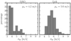 |
Fig. 1 Distribution of the uncertainties for the OAO and Lick RVs. The OAO data set has only 44 RVs, but they are slightly more precise than the 150 RVs from Lick. |
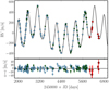 |
Fig. 2 Radial velocities for ν Oph along with their error bars measured at Lick Observatory are shown with blue circles covering more than 11 yr from July 2000 to October 2011. Green triangles denote the velocities from OAO, while the VLT near-IR data are plotted with red diamonds. The solid line illustrates the best dynamical model applied to the combined optical data from Lick and OAO. The near-IR data from VLT is only superimposed on the dynamical model with the only fitting parameter being an RV offset for the whole data set. The two wavelength domains are clearly consistent with each other. Bottom panel: residuals around the best fit. |
2.3 Stellar jitter
From our full Lick RV data set, we estimate the additional astrophysical RV noise around the best fit to be ~ 7.5 m s−1. In this paper, we adopt this short-term velocity scatter as stellar “jitter” (Wright 2005; Hekker et al. 2006). In fact, the same jitter level was estimated by Sato et al. (2012) using their OAO data set. This stellar jitter amplitude for ν Oph is typical for other late G and early K giants and is most likely due to rapid solar-like p-mode oscillations (Barban et al. 2004; De Ridder et al. 2006; Zechmeister et al. 2008), which appear as RV noise in our data. Based on the physical properties of ν Oph and the scaling relation from Kjeldsen & Bedding (1995), we estimate a scatter velocity of ~ 9 m s−1 and period of 0.27 d, which agrees well with our result from the RV data. In a more complete analysis, we could have left the jitter as a free parameter and estimated it together with the other system parameters, but as we are not interested in the exact value and an error estimate for the jitter term, we keep it fixed for simplicity. This is not expected to have a significant influence on any of the other results, as a reduced  would be the preferred outcome in any case.
3 Best fits
To model the orbital configuration of ν Oph we adopted a stellar mass of M = 2.7 M⊙ and we used all the available optical RV data for ν Oph. We combined our Lick RVs with those published in Sato et al. (2012), resulting in a total of 194 precise RVs with typical uncertainties of the order of 3–9 m s−1. For both data sets we quadratically added the estimated RV jitter of 7.5 m s−1 into the total error budget, and hence we considered the astrophysical stellar noise as an additional RV uncertainty. We analyzed the combined RV data by adopting the methodology described in Tan et al. (2013). We applied a Levenberg–Marquardt (LM)-based χ2 minimization technique coupled with two models, namely a double-Keplerian model and a self-consistent dynamical model with the equations of motion integrated using the Gragg–Bulirsch–Stoer integration method (Press et al. 1992). For both two-planet models the fitted parameters are the spectroscopic elements: RV semi-amplitude K, orbital period P, eccentricity e, argument of periastron ω, mean anomaly M0, and the RV data offset RVoff for each data set. All orbital parameters (including the derived semi-major axes a1, a2 and minimum masses m1 sin i, m2 sin i) are obtained in the Jacobi frame (e.g., Lee & Peale 2003) and are valid for the first observational epoch, which in our case is always JD 2451853.595 (the first Lick data point).
We further test our models for long-term dynamical stability using the SyMBA symplectic integrator (Duncan et al. 1998). The SyMBA integrator was modified to work directly with the obtained Jacobi elements as an input and we were able to simultaneously monitor the evolution of the orbital elements over time. Since we were aware that the companions period ratio is close to 6:1 we additionally monitored the evolution of the secular apsidal angle Δω = ω1 − ω2 and the evolution of all six resonance angles, defined as:
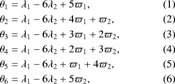
where ϖ1,2 = Ω1,2 + ω1,2 is the longitude of periastron and λ1,2 = M1,2 + ϖ1,2 is the meanlongitude of the inner and outer companion, respectively. Clearly, θ1…6 are not independent and can be derived from the evolution of one of the resonance angles and Δϖ. The expansion of all possible resonance angles, however, helps to identify the resonance angle θn with the lowest libration amplitude, which is an important dynamical characteristic of the system.
We start each orbital integration from JD = 2 451 853.595, and we collected orbital output from the simulations for every 10 yr of integration. The simulations were interrupted only in cases of mutual collisions between the companions and the star, or if one of the companions was ejected from the system. We defined an ejection as a case where one of the companions’ semimajor axes exceeds 10 AU during the integration time, and we defined a collision with the star as a case where the semimajor axis of one of the planets goes down to 0.1 AU. Since the age of the system is estimated to be ~ 0.65 Gyr, we integrate the individual best dynamical fits for a maximum of 1 Gyr, which gave us more than enough time to study the long-term stability of the system. For our stability test we adopted a time step equal to 2 days leading to about ~260 steps per complete orbit of the inner companion. We find that the selected time step was adequate to assure the precise simulation of the ν Oph system.
Best coplanar fits for the combined data sets of ν Oph.
3.1 Coplanar edge-on fit
The best Keplerian fit to the full optical data set has  and is clearly consistent with two massive companions in the brown dwarf regime with m1 sin i = 22.2 MJup and m2 sin i = 24.7 MJup. The orbits are noncircular with e1 = 0.124 ± 0.003 and e2 = 0.180 ± 0.006, respectively. The inner companion has an orbital period of P1 = 530.0 ± 0.1 d, while the outer companion has P2 = 3183.0 ± 5.9 d, consistent with the earlier findings by Quirrenbach et al. (2011) and Sato et al. (2012). Orbital parameters and uncertainties estimated from the covariance matrix for our best Keplerian fit are given in Table 2.
We use the best Keplerian model as a good initial guess for our dynamical fitting. The available RV data cover a bit more than one full period of the outer companion, and thus any mutual perturbations between the companions should be barely noticeable in the data. Indeed, despite both companions having large masses in the brown dwarf regime, they are too far separated in space to mutually influence their orbits strongly on short timescales. We thus find the difference between a double Keplerian and self-consistent two-planet edge-on dynamical model to be minor and insignificant. As can be seen from Table 2 both edge-on models mutually agree within the estimated errors, and therefore we conclude that there is little advantage to using an N-body model over the simpler double Keplerian. However, since our goal in this paper is to explore the long-term dynamical orbital evolution of the ν Oph system for coplanar edge-on and inclined configurations, we present results based on the dynamical model.
The best coplanar edge-on dynamical fit to the combined Doppler data has  and leads to orbital elements of P1 = 530.21 ± 0.10 d, P2 = 3184.83 ± 5.93 d, e1 = 0.124 ± 0.003, and e2 = 0.180 ± 0.006, and estimated masses of m1 = 22.2 MJup and m2 = 24.7 MJup. This fit also suggests that the ν Oph system is inan aligned orbital configuration with well constrained arguments of periastron ω1 = 9.9° ± 1.5° and ω2 = 8.3° ± 2.0°. The other orbital elements and their estimated parameter errors for this fit are listed in Table 2.
An illustration of the best coplanar edge-on dynamical fit to the ν Oph RV data sets is given in Fig. 2. Both data sets cover more than 11 yr of observations, which is slightly more than 1.25 orbital periods of the outer companion. In addition, the near-IR RVs from CRIRES taken by Trifonov et al. (2015) at later epochs are shown in Fig. 2 with red diamonds. The near-IR data points were superimposed on the best fit from the visible-light data, fitting only an RV offset for the whole near-IR data set. We use these data only to demonstrate the consistency between the two wavelength domains, but we did not use them in the orbital analysis.
The long-term dynamical simulation of the edge-on N-body fit shows that the system is stable and is indeed locked in a 6:1 MMR with all six resonant angles θ1–θ6 librating around 0°. Figure 3 shows a 50 kyr zoom from the 1 Gyr dynamical evolution of the best coplanar edge-on dynamical fit. The left panel from top to bottom illustrates the evolution of the semimajor axes (a1, a2), eccentricities (e1, e2), and the secular apsidal angle Δω = ω1 − ω2 of the brown dwarfs. Clearly, the semimajor axes do not exhibit any notable variations for 50 kyr and we find that this is also the case for the complete orbital simulation time of 1 Gyr. During the orbital evolution the semimajor axes oscillate with very low and regular amplitude around a1 ≈ 1.8 AU and a2 ≈ 5.9 AU, while the orbital eccentricities oscillate in an off-phase fashion. The inner brown dwarf has a mean orbital eccentricity of e1 ≈ 0.11, varying between 0.09 and 0.13, while the outer exhibits a lower eccentricity amplitude between 0.18 and 0.19 with a mean of e2 ≈ 0.185. The secular resonance angle Δω clearly librates around 0° with a semiamplitude of about 20°, showing that the system remains in an aligned configuration during the dynamical test. The middle and the right panels of Fig. 3 show the evolution of the resonant angles θ1, θ2, θ3 (from top to bottom) and θ4, θ5, θ6, respectively. For the best dynamical fit the largest semi-amplitude has Δθ1 = 105.3°, followed by Δθ2 = 86.0°, Δθ3 = 66.8°, Δθ4 = 47.6°, and the smallest libration semi-amplitude is at Δθ5 = 28.9°. The last resonant angle Δθ6 librates with a semi-amplitude of 37.3°, out of phase with respect to θ1 –θ5. The resonant libration period of the eccentricities and all resonance angles is about ~ 7 kyr, while these also exhibit lower amplitude and very regular short-period variations.
We note that the pattern depicted in Fig. 3, with θ5 having the smallest libration amplitude of all resonance angles, and a phase reversal between θ5 and θ6, is observed robustly over the parameter space that we have investigated. This behavior therefore provides a constraint on the resonance capture mechanism, which must be reproduced by models of the early evolution of the system.
3.2 Coplanar inclined configurations
For our coplanar inclined fitting we always fixed ΔΩ = 0° and set i1 = i2 = i. In this way, we keep the orbits in the same plane, and mutually inclined configurations are not allowed to occur. While fitting we only alter the line of sight inclination i of the system, together with all other Keplerian parameters (P, K, e, ω, M0). We obtained a best fit around i = 16°, which has a slightly lower  value when compared to the edge-on case, but we also estimated very large inclination uncertainties for this fit. This shows that there are only small, barely significant differences between coplanar edge-on and inclined dynamical fits, and we cannot constrain the orientation of the orbits from the current RV data. Thus, in our analysis we did not simply allow i to vary as a free parameter, but we tested a set of coplanar fits as a function of inclination. We started with our best edge-on dynamical fit at i = 90° (see Fig. 2 and Table 2) and for the sequence of fits we adopted a step of Δi = −1°. The minimum coplanar inclination we tested was at i = 3°, since a lower inclination leads to very massive companions approaching low-mass MS stars and above. Moreover, we find that N-body models with very low inclinations have large χν values (over 3σ from the best fit), so there was no reason to study inclinations lower than i < 3°.
Figure 4 illustrates the results from the coplanar inclined test. The red dots represent the dynamical models obtained from the combined data set and their  values plotted versus the inclination i. The red dashed lines represent 1σ, 2σ, and 3σ levels obtained from Δχ2 confidence values of 1.0, 4.0, and 9.0 larger than the χ2 minimum and scaled accordingly by the number of the degrees of freedom (d.o.f.) to match the
  levels in Fig. 4. Clearly, this test reveals that there is no significant
  minimum, although slightly better fits can be obtained between i ~ 10° and 30°. All these fits, however, are within 1σ from the coplanar edge-on fit and as such the improvement can be considered to be insignificant. Inclinations lower than i ~ 10° lead to models with rapidly increasing
  values, and these are generally not consistent with the data. We conclude that the dynamical fitting to the combined data is not sensitive to inclinations larger than i = 5° (at 3σ), but such nearly face-on configurations are statistically strongly disfavored. The global minimum appears to be at i = 16°, consistent with the best fit where we allowed the system’s line of sight inclination to be a free parameter. The obtained orbital parameters and their errors from the best coplanar inclined fit to the combined RV data are given in Table 2.
Despite the large companion masses obtained at i = 16°, this fit is stable for 1 Gyr and it has a similar 6:1 resonant orbital evolution to the coplanar edge-on case shown in Fig. 2. The difference in this case, however, is that all resonant angles evolve with higher frequency and larger libration amplitudes around 0°. The secular apsidal angle for this fit librates with a semi-amplitude of 34.9°, and the resonant angles’ libration semi-amplitudes are as follows: Δθ1 = 169.1°, followed by Δθ2 = 134.4°, Δθ3 = 99.7°, Δθ4 = 65.0°, Δθ5 = 32.2°, and Δθ6 = 49.2°.
Seeing that no confident constraints on the line of sight inclination can be made based on the combined data, we were motivated to repeat the same test, but using Lick and OAO data, separately. The idea was to see if the individual data sets contain any information that can help us to define the inclination, and whether these sets are mutually consistent. Figure 4 illustrates the same test applied to the Lick data in blue, and in green results from the OAO data. Individual dynamical models on both Lick and OAO data have different quality in terms of χ2 as they have a different overall velocity precision (see Fig. 1). Thus, in Fig. 4 their  curves and Δχ2 confidence levels are above (OAO data) and below (Lick data) the statistics from the combined data set. For the Lick data the minimum at i = 7° is significant at the 2σ level indicating that an inclined solution is slightly preferred, while the OAO data are not sensitive to inclination in the range i = 20°–90°.
In summary, we conclude that the slight preference for a rather low inclination (near i = 16°) is not statistically significant. The implied companion masses near or even above the hydrogen burning limit would in fact make the system evenmore perplexing, as discussed in Sect. 6.2.
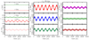 |
Fig. 3 Best coplanar edge-on orbital evolution shown for 50 kyr from the numerical simulation. Left panel, from top to bottom: orbital evolution of the companions’ semimajor axes, eccentricities, and the secular apsidal angle Δω. Clearly no change in a1 and a2 can be seen, while e1 and e2 are librating in opposite phase with small amplitudes. Other panels: resonance angles θ1,2,3 and θ4,5,6, which are clearly librating around 0° indicating the resonant nature of the system. See text for more details. |
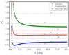 |
Fig. 4 Resulting |

4 Error estimation
4.1 χ2 statistics
Error estimation plays an essential role in our orbital analysis, since it helps to judge the reliability of the best-fit orbital parameters and to reveal the orbital configurations that agree with the data within the statistical significance limits. The individual best-fit parameter errors for ν Oph in Table 2 are obtained directly from the χ2 fitting using the covariance matrix ( ). These estimates represent symmetric 1σ uncertainties of the best-fit parameters. As can be seen from Table 2, the ν Oph system is very well constrained with estimated orbital uncertainties usually below 1%. As discussed in Sect. 3 we fit only the spectroscopic elements, and therefore the errors in physical parameters such as semimajor axes (a1,2) and companion masses (m1,2) must be obtained through additional error propagation. No errors in i1,2 and ΔΩ are obtained since our dynamical model to the RV data was unable to provide an adequate constraint for these orbital parameters. Instead, while fitting we always keep i1,2 and ΔΩ fixed.
Another method to estimate the orbital uncertainties from the RV data is based on constant Δχ2 boundaries. This method allows to explore the χ2 surface as a function of the fitting parameters, and as a result an overall χ2 confidence statistics can be obtained (see Ford 2005). The constant Δχ2 boundaries method is not practicable for models with a large number of free parameters (e.g., two-planet models), due to the large computational resources needed to evaluate a smooth χ2 surface in the multi-dimensional parameter space. However, if there are only one or two parameters of interest, the Δχ2 technique can be a fast and valuable tool for estimating the parameter uncertainties.
For example, when there is only one free parameter, the values of Δχ2 = 1.0, 4.0, 9.0 larger than the global  minimum will correspond to the 1σ, 2σ, and 3σ confidence levels, while if there are two parameters, the Δχ2 values will be 2.3, 6.2, and 11.8. As demonstrated in Sect. 3.2 and Fig. 4, the Δχ2 boundaries technique can be used effectively to constrain the significance of the line of sight inclination i for our dynamical models. In Fig. 4 for each studied data set with d.o.f., we draw the 1σ, 2σ, and 3σ levels, which correspond to
  confidence values of 1.0/d.o.f., 4.0/d.o.f., and 9.0/d.o.f. larger than the
  minimum. We note that these Δχ2 boundaries provide the correct statistics only if the applied model results in a minimum
 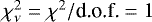 . None of our
  extrema for the three cases shown in Fig. 4 are actually exactly at unity, but they are close enough to consider the confidence levels as valid.
4.2 Bootstrap sampling
Apart from the covariance matrix and the Δχ2 statistics, it is possible to carry out an independent error estimation and to validate the uncertainties of the orbital elements by applying a bootstrap resampling of the original RV data. This method uses synthetic data sets, each of which can be fitted with a Keplerian or dynamical model, so that an overall statistical distribution of the fitted parameters can be obtained.
We followed the bootstrap prescription described in Press et al. (1992) and Tan et al. (2013). Briefly, for each data set containing N data points, we generated 5000 synthetic samples containing N data points, chosen randomly from the original data set with replacement. The OAO and Lick data sets were re-sampled separately and then combined. To each alternative combined data set we fitted a two-planet dynamical model and tested for stability as defined in Sect. 3. The sampling distribution of the fitted orbital parameters obtained with the bootstrap method for the edge-on coplanar configuration are illustrated in Fig. 5. We also show the distribution of the derived semimajor axes (a1, a2) and the companion masses (m1, m2). Since all simulated fits appeared to be stable (tmax = 10 Myr), Fig. 5 also shows the distribution of the libration semi-amplitudes for all six resonance angles (θ1 – θ6).
In Fig. 5, we also provide a comparison between the errors estimated from the covariance matrix of the best fit to the original data, and the 1σ confidence interval from the bootstrap distribution. In all plots, blue dots represent the best-fit values obtained from the best dynamical fit, while red error bars are the estimated uncertainties from the covariance matrix (see Table 2). We find that all best-fit parameters and their errors are consistent with the bootstrap distribution peak and the 68.3% confidence level (vertical dashed lines on Fig. 5). The bootstrap distribution is very symmetrical for all fitted parameters, and can be approximated well with a normal distribution.
5 Dynamical analysis
The statistical and dynamical properties of the fits within the statistically permitted region of the parameter space around the best fit can be obtained using a systematic  grid-search technique coupled with dynamical fitting, as was previously demonstrated in Lee et al. (2006), Tan et al. (2013), and Trifonov et al. (2014). To study the possible orbital configurations for the ν Oph system, we select pairs of parameters and construct high-density 2D grids consisting of 50 × 50 points for each of them. For each point on the grid, we keep these two parameters fixed, and perform a
  minimization with a dynamical model, allowing all other parameters to vary. By performing 50 × 50 dynamical fits, we thus obtain
  contours in the plane of the two chosen grid parameters. From these, we derive 1σ, 2σ, and 3σ confidence levels based on the Δχ2 statistics. As a final step, we integrate these fits for 10 Myr with SyMBA to study their stability and dynamical evolution.
5.1 Coplanar configurations
In an attempt to better understand the resonant nature of the ν Oph system, and to see if the resonance configuration of the system is preserved across the orbital phase space allowed by  , we constructed three different 2D coplanar edge-on grid combinations. We start with a grid, where we fix the period ratio P2 ∕P1 and the period of the inner planet P1, and then we construct grids of P2 versus e2 and ω2 versus e2. For the first, we systematically vary P1 in the range between 526 and 534 d, while varying P2 in such a way that for each P1 the resulting P2∕P1 increases from 5.95 to 6.05 with a constant step of 0.002. We test the P2, e2 grid for P2 = 3130–3240 d and the ω2, e2 grid for ω2 = 0°–50°; for both grids e2 was varied in the range e2 = 0.15–0.23. For all grids we examine the statistical properties around the best achieved fit, the stability and orbital evolution, and we record the distribution of all orbital elements and the libration amplitudes.
Results from the P2∕P1, P1 grid are shown in Fig. 6, while results from the P2, e2 and e2, ω2 grids are shown in Figs. 7 and 8, respectively. These figures show the achieved  and the RV rms surface from these tests, along with the dynamical properties around the best fit in terms of the derived libration semi-amplitudes for Δω and all six resonant angles θ1 –θ6. We marked the best fit in the grid with a star, while red contours trace the 1σ, 2σ, and 3σ significance levels in the grid obtained from Δχ2 statistics. We note that in all cases the chosen parameter ranges are sufficiently large for the grids to encompass the full 3σ contours.
We find that all studied combinations lead to similar conclusions; we summarize these as follows. All studied fits are stable for 10 Myr, and therefore no stability borders exist on these grids. The best fits found on the individual grids (black star symbol) are near the 6:1 period ratio and exhibit very similar orbital parameters and evolution when compared with the best coplanar edge-on dynamical fit shown in Table 2. Small differences occur in the fixed parameters, but that is expected given the finite resolution of the examined grids. We conclude that the best fits for all three grids are associated with the best coplanar edge-on fit for ν Oph and no other local  minima exists on the studied grids. The RV rms contours are consistent with the
  surface. We see lower rms values around the best fit, and the rms level smoothly increases between the best fit and the 3σ level. From these grids we find that all the 6:1 MMR resonance angles librate within the 3σ level and beyond, meaning that all significant fits in these grids are in 6:1 MMR. Figures 6–8 show that the resonance angle semi-amplitudes at the best fit are in very good agreement with those derived from the orbital evolution of the best coplanar edge-on fit illustrated in Fig. 3. It is clear, however, that all resonance angles have a minimum in libration amplitude (red ⊙ symbol on the figure subplots) different form the best fit. This amplitude minimum appears to be on the exact 6:1 period ratio, but over 3σ away from our best fit. This means that a deeper resonance state does exist for this system, but is not consistent with the data.
For many fits in the outer regions of the grids, all resonance angles circulate, and thus these fits are not associated with a MMR behavior. Nevertheless, looking at the subplots for Δω in all three grid combinations, one can see that Δω actually almost never circulates, and the system remains in an aligned geometry. This result suggests that these phase-space regions are not random, but the system is involved in secular interactions where Δω librates around 0°. We find that the libration amplitude of Δω depends on the initial Δω from which we start the numerical integrations. In the case of P2∕P1, P1 and P2, e2 grids, ω1 and ω2 are floating, and usually the best fit suggests nearly aligned orbital geometry. In the case of the e2, ω2 grid, ω2 is fixed between 0° and 50°, and the initial Δω can reach ≳ 30°. For such initial values we find that Δω circulates.
However, the grid regions where all the resonance angles circulate have very large  values, and thus such fits are statistically very unlikely to explain the ν Oph RV data. It is nevertheless interesting to investigate whether these fits are long-term stable over ~ 1 Gyr. We test a number of these cases for each gridin the region where the
  is larger (usually at the grid corners), and we find that even non-MMR orbital configurations are stable for 1 Gyr. We conclude that a large region of parameter space around the best fit contains only stable configurations, meaning that no stability constraints on the possible orbital configurations can be obtained for edge-on and coplanar orbits.
We repeated the P2∕P1 versus P1, P2 versus e2, and e2 versus ω2 grids for inclined coplanar configuration where we set i = 30°. In this way, we obtained approximately a factor of two times more massive companions for each fit. We find, however, that doubling the companion masses has little influence on  , and the RV rms grid contours resemble those for i = 90°. This result is not very surprising given the results presented in Fig. 4. Similar to the edge-on case the
  minimum on all grids matches with the best fit for i = 30° from the coplanar inclined test performed in Sect. 3.2.
The main goal for this test was to examine the resonance state of the ν Oph system assuming more massive bodies in orbit. We find that the test carried out for i = 30° is almost identical with the edge-on case. All grid points led to stable solutions, and the fits within the 3σ confidence contours are all in 6:1 MMR. The resonant regions on the grids had somewhat smaller surface area when compared to the edge-on case, but they exhibit similar libration amplitudes, while the libration frequency is higher as can be expected for more massive interacting bodies.
These results show that the ν Oph system is deeply trapped in a 6:1 MMR, and that this configuration is dynamically possible for a relatively large range of companion masses.
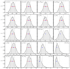 |
Fig. 5 First two columns: sampling distribution of all fitting parameters (K, P, e, ω, M) for a coplanar and edge-on configuration constructed from 5000 bootstrap samples. All bootstrap samples are stable for 10 Myr. Third and fourth columns: derived distribution of companion masses (m) and semimajor axes (a), and the libration semi-amplitudes of the resonance angles (θ1–θ6). The bluedots are the location of the best dynamical fit in phase space for both companions. The red error bars are the uncertainties estimated from the covariance matrix, while the errors in a and m are obtained through error propagation from these uncertainties. Clearly, for all orbital elements the best-fit values and their errors from the covariance matrix are consistent with the bootstrap distribution peak and the corresponding 68.3% confidence level (vertical dashed lines). |
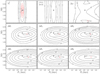 |
Fig. 6 Results from the P2∕P1 vs. P1 grid constructed from coplanar edge-on dynamical fits. The separate panels are self-explanatory: Top-left panel: |


5.2 Mutually inclined configurations
We investigated the hipparcos Intermediate Astrometric Data for ν Oph in an attempt to set constraints on the inclinations and the ascending nodes of the system as was demonstrated in Reffert & Quirrenbach (2011). We found that all but the lowest inclinations (down to about i1,2 = 5°) for both companions are consistent with the hipparcos data, while Ω1 and Ω2 are practically unconstrained. Therefore, no meaningful constraints on the orbital configuration could be derived from the hipparcos astrometry.
Although our dynamical fits to the RV data are also unable to constrain the orbital orientation, we test a large number of mutually inclined configurations by constructing grids of i1 versus i2. These grids are made in the range i1,2 = 5–175°, meaning that each step corresponds to δi1,2 = 3.4°. The mutual inclination, however, depends also on the difference between the orbital ascending nodes ΔΩ = Ω1 − Ω2:
 (7)
(7)
Therefore, we create a total of 12 i1, i2 grids with fixed values for ΔΩ = 0°, 30°, 60°, …, 330°. These grids cover a large set of mutually inclined configurations in the range Δi = 0–180°; from coplanar edge-on to highly inclined and retrograde orbits. For each set of i1, i2 and ΔΩ we apply our dynamical fitting routine and collect the  value and the best-fit orbital elements. For all fits obtained on these grids we test the long-term orbital evolution for 1 Myr.
Figure 9 visualizes the results from our i1, i2 versus ΔΩ grids. The red contours show the 1σ, 2σ, and 3σ levels measured from the global best-fit model on the grids of i1, i2 versus ΔΩ. The dashed contours mark the initial mutual inclination, in steps of Δi = 30°, obtained with Eq. (7) from i1, i2 and the given ΔΩ. Gray filled regions show the fits stable for at least 1 Myr.
For the grid with ΔΩ fixed at 0°, the mutual inclination only depends on Δi = |i1 − i2|, and therefore all coplanar inclined configurations are located on the diagonal with i1 = i2. The fits located on this diagonal are a repetition of the test performed in Sect. 3.2 and shown in Fig. 4 for the combined RV data set. In agreement with the results presented in Sect. 3.2, the coplanar inclined fits on this grid are all stable. The same is true for a large fraction of mutually inclined fits with Δi ≲ 45°. The best stable fits located within the 1σ confidence region on the grid, however, are located at i1 ≲ 15° or i1 ≳ 165° (i.e., sin i1 ≲ 0.26), where the inner companion is in the low-mass stellar range. This stable region covers a more extended range of mutual inclinations from configurations with Δi ≈ 30° and large companion masses to about Δi ≈ 100°, where the outer companion has a mass close to its minimum, while the inner companion mass is near its maximum on the grid. Additionally, two small stable regions exist for inclined configurations with Δi ≳ 150° (which is equivalent to Δi ≲ 30° with retrograde orbits), but these are over 2σ away from the best fit. The large S-shape stable island for ΔΩ = 0° gives a large range of companion masses and mutually inclined configurations that can explain the ν Oph system rather well.
The case for ΔΩ fixed at 30° shows a similar stable region to the case of ΔΩ = 0°, but with χν confidence contours suggesting decreasing quality of the fits in the stable region. Only one well-defined 1σ region is found in this grid, and almost all fits within it are stable. These fits are located at i1 ≳ 150° covering Δi between 10° and 90°. All other fits in the stable S-shape region are more than 1σ away from the best fit.
For ΔΩ = 60°, 90°, and 120°, the grids contain only configurations with high mutual inclinations, some with mostly prograde, others with mostly retrograde orbits. This has a major impact on the stable regions and the confidence contours. For these three grids the stable solutions are mostly located near the corners, corresponding to high-mass companions with relatively small prograde or retrograde mutual inclinations. The quality of these fits indicates that almost all of them are not within the 1σ region. For ΔΩ = 60°, the 1σ contours are rather similar to those at ΔΩ = 30°, but the central part of this grid has only a few stable fits, which in fact will most likely turn out to be unstable if tested for more than 1 Myr. The grids for ΔΩ = 90° and ΔΩ = 120° consist mostly of nearly perpendicular geometries, and the fits in the central 2σ regions are nearly all unstable. The large unstable regions at high mutual inclination in these and the other panels are most likely due to Kozai–Lidov cycles, which seem to affect the system stability.
A large stable region begins to emerge at very high mutual inclinations (Δi ≳ 150°) at ΔΩ = 150°. For ΔΩ = 180°, this stable region is well defined around the coplanar and retrograde diagonal at Δi = 180°. The fits at the central part for ΔΩ = 150° and 180° are close to the 1σ confidence level. Clearly, for retrograde orbits the system is only stable within relatively small limits of ≲ 30° for the mutual inclination (i.e., Δi ≳ 150°).
The panels in Fig. 9 for ΔΩ = 210°–330° are very similar to those for ΔΩ = 30°–150° (in reverse order). This is expected, as the transformation (i1,2 → 180° − i1,2, ΔΩ →−ΔΩ) leads to a system that is observationally indistinguishable and has the same stability properties. The small differences between the corresponding panels are due to numerical noise.
If the ν Oph system has indeed mutually inclined orbits, then most likely the system exists with relatively low mutual inclinations in prograde orbits, or even lower mutual inclination in retrograde orbital motion. Apart from cases in very small areas of parameter space, mutual inclinations with Δi between 60° and 150° lead to instability on very short timescales, due to the Kozai–Lidov effect. We caution, however, that the apparently stable regions might become smaller if longer integrations are carried out for the stability tests.
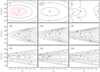 |
Fig. 7 Results from the P2 vs. e2 grid constructed from coplanar edge-on dynamical fits. The nine panels show contours for the same quantities as those in Fig. 6. |
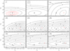 |
Fig. 8 As in Figs. 6 and 7, but for e2 vs. ω2. All fits on this grid are stable for at least 10 Myr, and the fits within the formal 3σ confidence level are in 6:1 MMR with θ1–θ6 librating around 0°. See text for details. |
6 Discussion
6.1 The nature of the brown dwarf desert
In 2003 the Working Group on Extrasolar Planets of the International Astronomical Union adopted a working definition according to which a substellar companion to a star is to be referred to as a planet if its mass is less than 13 MJup, and as a brown dwarf if its mass is higher (Boss et al. 2007). The main purpose of this distinction is the introduction of an unambiguous nomenclature that is closely linked to an observable quantity, although in the case of RV measurements the sin i ambiguity remains. The boundary at 13 MJup is motivatedby the deuterium burning limit, but from the point of view of companion formation mechanisms it is completely arbitrary.
Nevertheless, the distinction between planets and brown dwarf companions took on a second meaning with the realization that very few ~ 1 M⊙ main sequence stars harbor companions in the range 5–80 MJup, with orbital periods up to a few years (Marcy & Butler 2000). This brown dwarf desert can be understood as a deep minimum in the companion mass function between the planetary and stellar mass ranges (Grether & Lineweaver 2006), related to different formation mechanisms: whereas binary stars form in a cloud fragmentation process favoring pairs with nearly equal masses and thus a companion mass function with a positive slope, planets form in circumstellar disks, with a mass function with negative slope over the range considered here (gas giants with m ≳ 1 MJup). In this picture, the location of the minimum between the two companion mass functions in the range between the deuterium and hydrogen mass-burning limits is coincidental, but it provides a tentative connection between the mass-based nomenclature and the putative formation channels.
The large RV exoplanet surveys carried out during the past few decades have also discovered a fair number of companions with m sin i in the brown dwarfrange (e.g., Nidever et al. 2002; Patel et al. 2007; Sahlmann et al. 2011; Wilson et al. 2016). For some of these objects it has been possible to detect the astrometric signature of the orbital motion in the intermediate data of the hipparcos mission, and thus to measure sin i. In most cases, this has led to the realization that the secondaries are low-mass stars in nearly face-on orbits (e.g., Halbwachs et al. 2000; Sahlmann et al. 2011; Wilson et al. 2016), but a few true brown dwarf companions have also been confirmed in this way (Sozzetti & Desidera 2010; Reffert & Quirrenbach 2011). RV follow-up of transiting Jupiter-sized objects is an alternative way to firmly establish brown dwarf companions, as in the case of CoRoT-3 b (Deleuil et al. 2008).
Brown dwarf candidates have also been discovered in orbits around late G and K giants (e.g., Liu et al. 2008; Mitchell et al. 2013; Reffert et al. 2015), in addition to the two objects that are the subject of this paper. As the giant star surveys probe stellar masses up to ~ 4 M⊙, they may help to answer questions about the properties of the brown dwarf desert. One might for instance suspect that the characteristic mass of the desert (i.e., the mass at which the planetary and stellar-companion mass functions intersect) increases with the mass of the host star. This would be expected if the masses of planet-forming circumstellar disks increase with the stellar mass (e.g., Pascucci et al. 2016), and if the occurrence rate of stellar binaries depends on the mass ratio q rather than the absolute mass of the secondary (Chabrier et al. 2014; see also the region a ≤ 5 AU of Fig. 2 in Jumper & Fisher 2013).
The mass dependence of the brown dwarf desert seems to be borne out by comparing the numbers of brown dwarfs in RV surveys of main sequence stars and of giants. For example, the Keck-HIRES data on 1624 F to M dwarf stars tabulated by Butler et al. (2017) contain only two companions with m sin i in the brown dwarf range (HD 16760 b with m sin i = 13.1 MJup and M = 0.78 M⊙, and HD 214823 b with m sin i = 19.2 MJup and M = 1.22 M⊙). In contrast, our survey sample of 373 giant stars contains four brown dwarfs (see Table 3). Taking these numbers at face value, the rate of incidence of brown dwarfs is nearly a factor of ten higher in the latter sample. The fact that all four companions have masses of roughly 20 MJup and orbit host stars of ~2 M⊙ or higher further supports the hypothesis that these objects represent the high-mass end of the planetary mass function, which is shifted towards higher masses for more massive host stars.
One must caution, however, that this is by no means a conclusive statistical analysis. In addition to the sin i ambiguity, such an analysis would have to address various selection effects that may affect the inferred companion rate: (1) for many surveys, there is no published information about the full underlying target sample. In those cases it is impossible to convert numbers of detections into occurrence rates, as additional unpublished companions may be contained in the full sample. The two examples above have been chosen because the full information of these surveys is available. (2) Essentially all large RV surveys have very uneven temporal sampling across the target stars, as the survey teams usually allocate additional observations to “promising” or “interesting” targets. This makes the companion-detection thresholds rather nonuniform. (3) The task of establishing reliable detection thresholds is further complicated by varying levels of “stellar noise” due to activity and oscillations, whose amplitudes are strongly correlated with the stellar parameters, in particular for evolved stars (e.g., Hekker et al. 2006). (4) To analyze companion occurrence rates as a function of host star mass, these masses must be determined in the first place. This is not a trivial task in the case of giant stars (Stock et al. 2018). (5) The occurrence rate of massive planets depends not only on mass, but also on metallicity (Fischer & Valenti 2005; Reffert et al. 2015). While neglecting this dependency may lead to erroneous conclusions, attempts to determine the occurrence rate of rare objects (such as brown dwarfs) as a function of both parameters suffer strongly from low-number statistics.
The resolution of these problems will likely have to wait for the release of the epoch astrometry data from the Gaia mission. A 10 MJup companion in a 1 AU orbit around a 2 M⊙ star at a distance of 100 pc induces an astrometric motion of the host star with a 50 μas amplitude, which should be readily detectable by Gaia. The mission will thus conduct a complete census of brown dwarf companions to thousands of A and F main sequence stars. For the time being, the double-brown dwarf system ν Oph provides additional insights into the link between brown dwarfs and high-mass planets, as discussed in the following section.
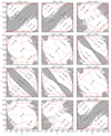 |
Fig. 9 Mutually inclined grids for different ΔΩ. The red contours illustrate the 1σ, 2σ, and 3σ confidence levels, while the black dashed lines delineate constant values of the initial mutual inclination Δi. The stability of the best-fit solution for each grid point is tested for 1 Myr, and gray filled contours show the grid areas where the orbits are stable. See text for details. |
Brown dwarf companions in the Lick giant star survey sample.
6.2 The formation of brown dwarf companions
Brown dwarf companions can in principle form through three different mechanisms: (1) turbulent fragmentation of a molecular cloud (Bate 2012; Luhman 2012), as in the case of a binary star with very high mass ratio; (2) fragmentation of the disk during the formation of the primary (Stamatellos & Whitworth 2011; Kratter & Lodato 2016); and (3) core accretion, as in Jovian planets. Models of these processes predict different properties of the companion population, but they could all contribute to a varying extent in different sections of the parameter space, which makes it difficult to assess their relative importance (Marks et al. 2017). It would thus be highly desirable to firmly identify the formation mechanism for individual well-characterized objects. The ν Oph double-brown dwarf system is particularly suited to addressing this question, because its unusual properties place constraints on its formation pathway.
First we note that molecular cloud fragmentation into multiple “star”-forming cores is a very unlikely formation process for the ν Oph system. Thefinding that the two brown dwarfs are in a 6:1 MMR configuration is robust across virtually all of the allowed parameter space, for coplanar as well as mutually inclined orbits. No similar configuration is known for any multiple stellar system (Tokovinin 2018), whereas orbital resonances are rather common in planetary systems, and their presence is best explained by resonance capture during convergent migration of the planets forming in the circumstellar disk (e.g., Lee & Peale 2002; Kley & Nelson 2012). It is therefore very likely that the two brown dwarfs formed in the disk of ν Oph when it was a Herbig Ae star.
This leaves the question open as to whether disk fragmentation or core accretion is the more likely formation process. Unfortunately, we do not have access to the radii of the brown dwarfs, and therefore there are no constraints on their composition, which could potentially discriminate between the two scenarios and provide additional information on the disk properties (Guillot et al. 2014; Humphries & Nayakshin 2018). There is no agreement in the literature over the importance of gravitational instabilities in circumstellar disks for planet and brown dwarf formation. While, for example Chabrier et al. (2014) dismiss this mechanism as a major contributor to the companion population around single stars, others argue that disk fragmentation is responsible for most of the companions with high masses and/or large orbital radii (Stamatellos & Whitworth 2009; Schlaufman 2018; Vorobyov & Elbakyan 2018). In fact, Dodson-Robinson et al. (2009) investigated core accretion, scattering from the inner disk, and gravitational instability as potential formation scenarios; they conclude that only the last is a viable mechanism to form gas giants on stable orbits with semi-major axes ≳ 35 AU. Simulations of self-gravitating disk fragments by Forgan et al. (2015) produced some systems that bear a remarkable resemblance to ν Oph (see their Fig. 2). This would seem to argue that ν Oph b and ν Oph c formed by disk fragmentation. One should caution, however, that these studies considered mostly host stars with ~ 1 M⊙. If the maximum mass of 10 MJup postulated by Schlaufman (2018) for companions formed by core accretion scales with the host star mass, ν Oph b and ν Oph c may well fall below this limit.
Maldonado & Villaver (2017) investigate the dependence of brown dwarf formation on stellar metallicity and suggest that gravitational instability might be dominant at lower, and core accretion at higher values of the metallicity. Of the host stars to brown dwarfs in the Lick giant star survey sample (Table 3), 11 Com has a relatively low metallicity (rank 78/366 of all stars in Hekker & Meléndez 2007), whereas ν Oph and τ Gem have relatively high metallicities (rank 318 and 354/366, respectively). With this small number of objects it is thus not possible to attribute the occurrence of brown dwarf companions among the Lick sample to either high or low host star metallicity.
There may be an interesting direct link between the ν Oph system and planets in wide orbits found by direct imaging. For example, the HR 8799 system also appears to have formed in a massive disk, and it has been suggested that its configuration represents a chain of multiple MMRs (Fabrycky & Murray-Clay 2010; Goździewski & Migaszewski 2014; Wang et al. 2018). It thus appears plausible that both systems formed through fragmentation in the outer regions of the circumstellar disk (≳ 40–70 AU; Kratter et al. 2010) and subsequent inward migration and resonance capture. However, in this scenario one would expect an even larger population of similar objects with larger companion masses (Kratter et al. 2010; Murray-Clay 2010), which appears not to be the case for either the directly imaged planets or the companions of giant stars found in RV surveys.
To settle the question about the origin of ~20 MJup objects, better statistics and in particular more multiple systems are clearly needed. Since the number of giant stars accessible to RV observations with modest-size telescopes is far larger than the samples surveyed so far, additional examples may be found soon. At present, the system most similar to ν Oph in the literature is BD +20 2457, with two companions with masses of 12.5 MJup and 21.4 MJup orbiting at 1.4 and 2 AU, respectively (Niedzielski et al. 2009). This system can probably not be stable if it is not in an MMR, but so far attempts to find any such stable configurations have failed, casting some doubts on the reality of the companions (Horner et al. 2014; Trifonov et al. 2014). It would therefore be highly desirable to collect more data on this star.
Another system that bears some close resemblance to ν Oph is the 5:1 MMR system HD 202206, which contains a brown dwarf (m sin i = 16.6 MJup) and a giant planet (m sin i = 2.2 MJup) orbiting a 1.0 M⊙ star (Correia et al. 2005; Couetdic et al. 2010). The HD 202206 system can be explained by either formation of both brown dwarf and planet in a circumstellar disk, or formation of the star–brown dwarf binary and then formation of the planet in a circum-binary disk.
As a final remark we note that the true masses of ν Oph b and ν Oph c could be substantially larger than 20 MJup, perhaps even above the hydrogen burning limit, as discussed in Sect. 3. This would not invalidate any of the arguments about the formation scenarios, but in that case core accretion would not appear plausible, leaving disk fragmentation as the only viable formation mechanism.
7 Summary and conclusions
In this paper, we present results of an orbital analysis of the ν Oph system, which contains an evolved K-giant star with M = 2.7 M⊙ and two brown dwarf companions with minimum masses m1 sin i = 22.2 MJup for the inner companion, and m2 sin i = 24.7 MJup for the outer. It was previously known that this system is consistent with orbital periods close to 6:1 in ratio, and therefore we have performed a detailed study to decide if this system is indeed trapped in an MMR.
For our analysis we use 150 precise Lick Observatory Doppler measurements, which we obtained between 2000 and 2011. We combine our RVs with an additional 44 precise RVs from the OAO Observatory, available in the literature. The total of 194 data points have a mean precision of ~ 5 m s−1, but we quadratically added to the RV data uncertainties an additional estimated stellar jitter velocity of 7.5 m s−1. Finally, we model the combined data with self-consistent dynamical fits, which calculate ν Oph’s spectroscopic reflex motion by taking into account the mutual gravitational interactions between the bodies in the system.
Our best coplanar edge-on model to the combined data suggests that both orbits are aligned with arguments of periastron ω1 = 9.9° ± 1.5° and ω2 = 8.3° ± 2.0°, respectively. A long-term stability analysis reveals that the coplanar edge-on fit is stable for at least 1 Gyr, and that the system is deeply trapped in a 6:1 MMR. Our dynamical test reveals a very coherent orbital evolution, where the brown dwarf eccentricities librate with moderate amplitudes, while the variations of the semimajor axes are negligible. Close inspection of the long-term resonant state of the system shows that all six resonance angles θ1 –θ6 and the secular Δω are librating around 0°. We conclude that these results represent strong evidence for the ν Oph system being in a resonant configuration.
To verify the best edge-on coplanar model estimates for the ν Oph system we test a large number of synthetic RV data sets generated with a bootstrap technique. We find that the achieved bootstrap distribution of the orbital elements and their confidence levels are fully consistent with our best N-body edge-on fit and its error estimates. In a final stability test, we find that all bootstrap fits are stable for at least 10 Myr, and that all are in resonance.
We have also carried out a large number of coplanar inclined dynamical fits in the same way as in the edge-on case. The best inclined fit yields an inclination of i = 16°, leading to much larger companions masses, namely m1 = 82.0 MJup and m2 = 92.0 MJup. The remaining spectroscopic parameters for the best inclined fit, however, are very similar to those from the coplanar edge-on model and we find that both best-fit solutions agree within the 1σ uncertainties. Since the improvement in χ2 compared to the edge-on fit is insignificant, we conclude that with the current combined RV data set it is impossible to constrain the line of sight orbital inclination using a dynamical model. Remarkably, all coplanar inclined fits down to i = 5° are also stable and in 6:1 resonance. As expected, with increasing brown dwarf masses the system becomes more dynamically active: the resonance angles still librate around 0°, but with increasing libration amplitudes and frequencies. In these fits the companions remain well separated and retain a clear 6:1 period ratio during the integrations.
Finally, we study the  and stability of the system as a function of various orbital parameter combinations. We construct high-density 2D coplanar edge-on grids with P2∕P1 versus P1, P2 versus e2 and ω2 versus e2 as fixed parameters, which were systematically varied on the grids, while all other orbital parameters were allowed to vary freely. We selected the parameter pairs in such a way that we could study the fit properties out to at least a few σ away from the best fit. We find that all fits on these grids are stable for at least 10 Myr. The vast majority of these configurations are found to be in the 6:1 MMR. We repeat the 2D grid test for i = 30°, where the companion masses are doubled, and find similar results. Since the two companions are well separated, increasing the companion masses has little influence on the long-term stability.
We also construct 12 grids with mutually inclined orbits by adopting different ΔΩ. We conclude that moderate mutual inclinations in prograde orbits, or small mutual inclinations in retrograde orbits are stable. Except for a few isolated cases, mutual inclinations with Δi between 60° and 150° lead to instability on very short time scales, most likely due to Kozai-Lidov effects. We caution, however, that these stability tests were carried out only for 1 Myr, and that longer integrations might reduce the sizes of the stable regions.
In summary, we conclude that the K giant star ν Oph is orbited by two companions with minimum dynamical masses of m1 sin i = 22.2 MJup and m2 sin i = 24.7 MJup, which are locked in a 6:1 MMR. This conclusion is robust also if large inclinations with respect to the line-of-sight or even mutually inclined orbits are considered. It is very likely that the two brown dwarf companions formed in the disk of ν Oph when the system was young, but it is not possible at present to decide whether the mechanism was gravitational instability or core accretion.
Acknowledgements
We thank the staff of Lick Observatory for their excellent support over many years. David Mitchell, Saskia Hekker, Simon Albrecht, Christian Schwab, Julian Stürmer and all the graduate students that have spent many nights on Mt. Hamilton to collect spectra. Special thanks are due to Geoff Marcy, Paul Butler, and Debra Fischer for permission to use their equipment and software. T.T. and M.H.L. were supported in part by the Hong Kong RGC grant HKU 7024/13P.
Appendix A Additional table
Measured velocities for ν Oph and the derived errors.
References
- Barban, C., De Ridder, J., Mazumdar, A., et al. 2004, in SOHO 14 Helio- and Asteroseismology: Towards a Golden Future, ed. D. Danesy, ESA SP, 559, 113 [NASA ADS] [Google Scholar]
- Bate, M. R. 2012, MNRAS, 419, 3115 [NASA ADS] [CrossRef] [Google Scholar]
- Boss, A. P., Butler, R. P., Hubbard, W. B., et al. 2007, Trans. Int. Astron. Union Ser. A, 26, 183 [Google Scholar]
- Bryden, G., Różyczka, M., Lin, D. N. C., & Bodenheimer, P. 2000, ApJ, 540, 1091 [Google Scholar]
- Butler, R. P., Marcy, G. W., Williams, E., et al. 1996, PASP, 108, 500 [NASA ADS] [CrossRef] [Google Scholar]
- Butler, R. P., Marcy, G. W., Williams, E., Hauser, H., & Shirts, P. 1997, ApJ, 474, L115 [NASA ADS] [CrossRef] [Google Scholar]
- Butler, R. P., Vogt, S. S., Laughlin, G., et al. 2017, AJ, 153, 208 [NASA ADS] [CrossRef] [Google Scholar]
- Chabrier, G., Johansen, A., Janson, M., & Rafikov, R. 2014, Protostars and Planets VI (Tucson: University of Arizona Press), 619 [Google Scholar]
- Correia, A. C. M., Udry, S., Mayor, M., et al. 2005, A&A, 440, 751 [NASA ADS] [CrossRef] [EDP Sciences] [Google Scholar]
- Correia, A. C. M., Udry, S., Mayor, M., et al. 2009, A&A, 496, 521 [NASA ADS] [CrossRef] [EDP Sciences] [Google Scholar]
- Couetdic, J., Laskar, J., Correia, A. C. M., Mayor, M., & Udry, S. 2010, A&A, 519, A10 [NASA ADS] [CrossRef] [EDP Sciences] [Google Scholar]
- De Ridder, J., Barban, C., Carrier, F., et al. 2006, A&A, 448, 689 [NASA ADS] [CrossRef] [EDP Sciences] [Google Scholar]
- Deleuil, M., Deeg, H. J., Alonso, R., et al. 2008, A&A, 491, 889 [NASA ADS] [CrossRef] [EDP Sciences] [Google Scholar]
- Desort, M., Lagrange, A.-M., Galland, F., et al. 2008, A&A, 491, 883 [NASA ADS] [CrossRef] [EDP Sciences] [Google Scholar]
- Dodson-Robinson, S. E., Veras, D., Ford, E. B., & Beichman, C. A. 2009, ApJ, 707, 79 [NASA ADS] [CrossRef] [Google Scholar]
- Duncan, M. J., Levison, H. F., & Lee, M. H. 1998, AJ, 116, 2067 [NASA ADS] [CrossRef] [EDP Sciences] [Google Scholar]
- ESA 1997, The Hipparcos and Tycho catalogues. Astrometric and photometric star catalogues derived from the ESA Hipparcos Space Astrometry Mission, ESA SP, 1200 [Google Scholar]
- Fabrycky, D. C., & Murray-Clay, R. A. 2010, ApJ, 710, 1408 [NASA ADS] [CrossRef] [Google Scholar]
- Fischer, D. A., & Valenti, J. 2005, ApJ, 622, 1102 [NASA ADS] [CrossRef] [Google Scholar]
- Fischer, D. A., Vogt, S. S., Marcy, G. W., et al. 2007, ApJ, 669, 1336 [NASA ADS] [CrossRef] [Google Scholar]
- Ford, E. B. 2005, AJ, 129, 1706 [Google Scholar]
- Forgan, D., Parker, R. J., & Rice, K. 2015, MNRAS, 447, 836 [NASA ADS] [CrossRef] [Google Scholar]
- Frink, S., Quirrenbach, A., Fischer, D., Röser, S., & Schilbach, E. 2001, PASP, 113, 173 [NASA ADS] [CrossRef] [Google Scholar]
- Frink, S., Mitchell, D. S., Quirrenbach, A., et al. 2002, ApJ, 576, 478 [NASA ADS] [CrossRef] [MathSciNet] [Google Scholar]
- Girardi, L., Bressan, A., Bertelli, G., & Chiosi, C. 2000, A&AS, 141, 371 [NASA ADS] [CrossRef] [EDP Sciences] [Google Scholar]
- Goździewski, K., & Migaszewski, C. 2014, MNRAS, 440, 3140 [NASA ADS] [CrossRef] [Google Scholar]
- Grether, D., & Lineweaver, C. H. 2006, ApJ, 640, 1051 [NASA ADS] [CrossRef] [Google Scholar]
- Guillot, T., Lin, D. N. C., Morel, P., Havel, M., & Parmentier, V. 2014, EAS Pub. Ser., 65, 327 [CrossRef] [EDP Sciences] [Google Scholar]
- Halbwachs, J. L., Arenou, F., Mayor, M., Udry, S., & Queloz, D. 2000, A&A, 355, 581 [NASA ADS] [Google Scholar]
- Hekker, S., & Meléndez, J. 2007, A&A, 475, 1003 [NASA ADS] [CrossRef] [EDP Sciences] [Google Scholar]
- Hekker, S., Reffert, S., Quirrenbach, A., et al. 2006, A&A, 454, 943 [NASA ADS] [CrossRef] [EDP Sciences] [Google Scholar]
- Horner, J., Wittenmyer, R. A., Hinse, T. C., & Marshall, J. P. 2014, MNRAS, 439, 1176 [NASA ADS] [CrossRef] [Google Scholar]
- Humphries, R. J., & Nayakshin, S. 2018, MNRAS, 477, 593 [NASA ADS] [CrossRef] [Google Scholar]
- Izumiura, H. 1999, Publications of the Yunnan Observatory, 77 [Google Scholar]
- Johnson, J. A., Marcy, G. W., Fischer, D. A., et al. 2006, ApJ, 652, 1724 [NASA ADS] [CrossRef] [Google Scholar]
- Jumper, P. H., & Fisher, R. T. 2013, ApJ, 769, 9 [NASA ADS] [CrossRef] [Google Scholar]
- Kjeldsen, H., & Bedding, T. R. 1995, A&A, 293, 87 [NASA ADS] [Google Scholar]
- Kley, W. 2000, MNRAS, 313, L47 [NASA ADS] [CrossRef] [Google Scholar]
- Kley, W., & Nelson, R. P. 2012, ARA&A, 50, 211 [NASA ADS] [CrossRef] [Google Scholar]
- Kratter, K., & Lodato, G. 2016, ARA&A, 54, 271 [NASA ADS] [CrossRef] [Google Scholar]
- Kratter, K. M., Murray-Clay, R. A., & Youdin, A. N. 2010, ApJ, 710, 1375 [NASA ADS] [CrossRef] [Google Scholar]
- Lee, M. H., & Peale, S. J. 2002, ApJ, 567, 596 [NASA ADS] [CrossRef] [Google Scholar]
- Lee, M. H., & Peale, S. J. 2003, ApJ, 592, 1201 [NASA ADS] [CrossRef] [Google Scholar]
- Lee, M. H., Butler, R. P., Fischer, D. A., Marcy, G. W., & Vogt, S. S. 2006, ApJ, 641, 1178 [NASA ADS] [CrossRef] [Google Scholar]
- Liu, Y.-J., Sato, B., Zhao, G., et al. 2008, ApJ, 672, 553 [NASA ADS] [CrossRef] [Google Scholar]
- Luhman, K. L. 2012, ARA&A, 50, 65 [NASA ADS] [CrossRef] [Google Scholar]
- Maldonado, J., & Villaver, E. 2017, A&A, 602, A38 [NASA ADS] [CrossRef] [EDP Sciences] [Google Scholar]
- Marcy, G. W., & Butler, R. P. 2000, PASP, 112, 137 [NASA ADS] [CrossRef] [Google Scholar]
- Marcy, G. W., Butler, R. P., Fischer, D., et al. 2001, ApJ, 556, 296 [NASA ADS] [CrossRef] [Google Scholar]
- Marks, M., Martín, E. L., Béjar, V. J. S., et al. 2017, A&A, 605, A11 [NASA ADS] [CrossRef] [EDP Sciences] [Google Scholar]
- Mayor, M., & Queloz, D. 1995, Nature, 378, 355 [NASA ADS] [CrossRef] [Google Scholar]
- Mitchell, D. S., Frink, S., Quirrenbach, A., et al. 2003, BAAS, 35, 1234 [NASA ADS] [Google Scholar]
- Mitchell, D. S., Reffert, S., Trifonov, T., Quirrenbach, A., & Fischer, D. A. 2013, A&A, 555, A87 [NASA ADS] [CrossRef] [EDP Sciences] [Google Scholar]
- Murray-Clay, R. A. 2010, in New Horizons in Astronomy: Frank N. Bash Symposium 2009, eds. L. M. Stanford, J. D. Green, L. Hao, & Y. Mao, ASP Conf. Ser., 432, 98 [NASA ADS] [Google Scholar]
- Nidever, D. L., Marcy, G. W., Butler, R. P., Fischer, D. A., & Vogt, S. S. 2002, ApJS, 141, 503 [NASA ADS] [CrossRef] [Google Scholar]
- Niedzielski, A., Konacki, M., Wolszczan, A., et al. 2007, ApJ, 669, 1354 [NASA ADS] [CrossRef] [Google Scholar]
- Niedzielski, A., Nowak, G., Adamów, M., & Wolszczan, A. 2009, ApJ, 707, 768 [NASA ADS] [CrossRef] [Google Scholar]
- Ortiz, M., Reffert, S., Trifonov, T., et al. 2016, A&A, 595, A55 [NASA ADS] [CrossRef] [EDP Sciences] [Google Scholar]
- Pascucci, I., Testi, L., Herczeg, G. J., et al. 2016, ApJ, 831, 125 [NASA ADS] [CrossRef] [Google Scholar]
- Patel, S. G., Vogt, S. S., Marcy, G. W., et al. 2007, ApJ, 665, 744 [Google Scholar]
- Press, W. H., Teukolsky, S. A., Vetterling, W. T., & Flannery, B. P. 1992, Numerical Recipes in FORTRAN: The Art of Scientific Computing, 2nd edn. (Cambridge: Cambridge University Press) [Google Scholar]
- Quirrenbach, A., Reffert, S., & Bergmann, C. 2011, in Planetary Systems Beyond the Main Sequence, eds. S. Schuh, H. Drechsel, & U. Heber, AIP Conf. Ser. 1331, 102 [NASA ADS] [CrossRef] [Google Scholar]
- Reffert, S., & Quirrenbach, A. 2011, A&A, 527, A140 [NASA ADS] [CrossRef] [EDP Sciences] [Google Scholar]
- Reffert, S., Quirrenbach, A., Mitchell, D. S., et al. 2006, ApJ, 652, 661 [NASA ADS] [CrossRef] [Google Scholar]
- Reffert, S., Bergmann, C., Quirrenbach, A., Trifonov, T., & Künstler, A. 2015, A&A, 574, A116 [NASA ADS] [CrossRef] [EDP Sciences] [Google Scholar]
- Sahlmann, J., Ségransan, D., Queloz, D., et al. 2011, A&A, 525, A95 [NASA ADS] [CrossRef] [EDP Sciences] [Google Scholar]
- Sato, B., Ando, H., Kambe, E., et al. 2003, ApJ, 597, L157 [NASA ADS] [CrossRef] [Google Scholar]
- Sato, B., Omiya, M., Harakawa, H., et al. 2012, PASJ, 64, 135 [NASA ADS] [CrossRef] [Google Scholar]
- Schlaufman, K. C. 2018, ApJ, 853, 37 [NASA ADS] [CrossRef] [Google Scholar]
- Setiawan, J., Hatzes, A. P., von der Lühe, O., et al. 2003, A&A, 398, L19 [NASA ADS] [CrossRef] [EDP Sciences] [Google Scholar]
- Sozzetti, A., & Desidera, S. 2010, A&A, 509, A103 [NASA ADS] [CrossRef] [EDP Sciences] [Google Scholar]
- Stamatellos, D., & Whitworth, A. P. 2009, MNRAS, 392, 413 [Google Scholar]
- Stamatellos, D., & Whitworth, A. 2011, Eur. Phys. J. Web Conf., 16, 05001 [CrossRef] [Google Scholar]
- Stock, S., Reffert, S., & Quirrenbach, A. 2018, A&A, 616, A33 [NASA ADS] [CrossRef] [EDP Sciences] [Google Scholar]
- Tan, X., Payne, M. J., Lee, M. H., et al. 2013, ApJ, 777, 101 [NASA ADS] [CrossRef] [Google Scholar]
- Tokovinin, A. 2018, ApJS, 235, 6 [NASA ADS] [CrossRef] [Google Scholar]
- Trifonov, T., Reffert, S., Tan, X., Lee, M. H., & Quirrenbach, A. 2014, A&A, 568, A64 [NASA ADS] [CrossRef] [EDP Sciences] [Google Scholar]
- Trifonov, T., Reffert, S., Zechmeister, M., Reiners, A., & Quirrenbach, A. 2015, A&A, 582, A54 [NASA ADS] [CrossRef] [EDP Sciences] [Google Scholar]
- Valenti, J. A., Butler, R. P., & Marcy, G. W. 1995, PASP, 107, 966 [NASA ADS] [CrossRef] [Google Scholar]
- van Leeuwen, F. 2007, A&A, 474, 653 [NASA ADS] [CrossRef] [EDP Sciences] [Google Scholar]
- Vogt, S. S. 1987, PASP, 99, 1214 [NASA ADS] [CrossRef] [Google Scholar]
- Vorobyov, E. I., & Elbakyan, V. G. 2018, A&A, 618, A7 [NASA ADS] [CrossRef] [EDP Sciences] [Google Scholar]
- Wang, J. J., Graham, J. R., Dawson, R., et al. 2018, AJ, 156, 192 [NASA ADS] [CrossRef] [Google Scholar]
- Wilson, P. A., Hébrard, G., Santos, N. C., et al. 2016, A&A, 588, A144 [NASA ADS] [CrossRef] [EDP Sciences] [Google Scholar]
- Wright, J. T. 2005, PASP, 117, 657 [NASA ADS] [CrossRef] [Google Scholar]
- Zechmeister, M., Reffert, S., Hatzes, A. P., Endl, M., & Quirrenbach, A. 2008, A&A, 491, 531 [NASA ADS] [CrossRef] [EDP Sciences] [Google Scholar]
Main sequence: Mayor & Queloz (1995), Butler et al. (1997), Fischer et al. (2007) etc., Sub-giants: Johnson et al. (2006) etc., and Giants: Frink et al. (2001), Setiawan et al. (2003), Sato et al. (2003), Niedzielski et al. (2007), Reffert et al. (2015) etc.
All Tables
All Figures
|
Fig. 1 Distribution of the uncertainties for the OAO and Lick RVs. The OAO data set has only 44 RVs, but they are slightly more precise than the 150 RVs from Lick. |
| In the text | |
|
Fig. 2 Radial velocities for ν Oph along with their error bars measured at Lick Observatory are shown with blue circles covering more than 11 yr from July 2000 to October 2011. Green triangles denote the velocities from OAO, while the VLT near-IR data are plotted with red diamonds. The solid line illustrates the best dynamical model applied to the combined optical data from Lick and OAO. The near-IR data from VLT is only superimposed on the dynamical model with the only fitting parameter being an RV offset for the whole data set. The two wavelength domains are clearly consistent with each other. Bottom panel: residuals around the best fit. |
| In the text | |
|
Fig. 3 Best coplanar edge-on orbital evolution shown for 50 kyr from the numerical simulation. Left panel, from top to bottom: orbital evolution of the companions’ semimajor axes, eccentricities, and the secular apsidal angle Δω. Clearly no change in a1 and a2 can be seen, while e1 and e2 are librating in opposite phase with small amplitudes. Other panels: resonance angles θ1,2,3 and θ4,5,6, which are clearly librating around 0° indicating the resonant nature of the system. See text for more details. |
| In the text | |
|
Fig. 4 Resulting |
| In the text | |
|
Fig. 5 First two columns: sampling distribution of all fitting parameters (K, P, e, ω, M) for a coplanar and edge-on configuration constructed from 5000 bootstrap samples. All bootstrap samples are stable for 10 Myr. Third and fourth columns: derived distribution of companion masses (m) and semimajor axes (a), and the libration semi-amplitudes of the resonance angles (θ1–θ6). The bluedots are the location of the best dynamical fit in phase space for both companions. The red error bars are the uncertainties estimated from the covariance matrix, while the errors in a and m are obtained through error propagation from these uncertainties. Clearly, for all orbital elements the best-fit values and their errors from the covariance matrix are consistent with the bootstrap distribution peak and the corresponding 68.3% confidence level (vertical dashed lines). |
| In the text | |
|
Fig. 6 Results from the P2∕P1 vs. P1 grid constructed from coplanar edge-on dynamical fits. The separate panels are self-explanatory: Top-left panel: |
| In the text | |
|
Fig. 7 Results from the P2 vs. e2 grid constructed from coplanar edge-on dynamical fits. The nine panels show contours for the same quantities as those in Fig. 6. |
| In the text | |
|
Fig. 8 As in Figs. 6 and 7, but for e2 vs. ω2. All fits on this grid are stable for at least 10 Myr, and the fits within the formal 3σ confidence level are in 6:1 MMR with θ1–θ6 librating around 0°. See text for details. |
| In the text | |
|
Fig. 9 Mutually inclined grids for different ΔΩ. The red contours illustrate the 1σ, 2σ, and 3σ confidence levels, while the black dashed lines delineate constant values of the initial mutual inclination Δi. The stability of the best-fit solution for each grid point is tested for 1 Myr, and gray filled contours show the grid areas where the orbits are stable. See text for details. |
| In the text | |
Current usage metrics show cumulative count of Article Views (full-text article views including HTML views, PDF and ePub downloads, according to the available data) and Abstracts Views on Vision4Press platform.
Data correspond to usage on the plateform after 2015. The current usage metrics is available 48-96 hours after online publication and is updated daily on week days.
Initial download of the metrics may take a while.