| Issue |
A&A
Volume 624, April 2019
|
|
|---|---|---|
| Article Number | A64 | |
| Number of page(s) | 14 | |
| Section | Planets and planetary systems | |
| DOI | https://doi.org/10.1051/0004-6361/201834357 | |
| Published online | 11 April 2019 | |
High resolution optical spectroscopy of the N2-rich comet C/2016 R2 (PanSTARRS)
1
ESO (European Southern Observatory),
Alonso de Cordova 3107,
Vitacura, Santiago, Chile
e-mail: This email address is being protected from spambots. You need JavaScript enabled to view it.
2
STAR Institute, University of Liège,
Allée du 6 Août 19c,
4000 Liège, Belgium
3
Institut UTINAM-UMR CNRS 6213, Observatoire des Sciences de l’Univers THETA, University of Franche-Comté,
BP 1615,
25010 Besançon Cedex, France
4
Oukaimeden Observatory, High Energy Physics and Astrophysics Laboratory, Cadi Ayyad University, Marrakech, Morocco
Received:
1
October
2018
Accepted:
24
January
2019
Abstract
Context. Early observations of comet C/2016 R2 (PanSTARRS) have shown that the composition of this comet is very peculiar. Radio observations have revealed a CO-rich and HCN-poor comet and an optical coma dominated by strong emission bands of CO+ and, more surprisingly, N2+.
Aims. The strong detection of N2+ in the coma of C/2016 R2 provided an ideal opportunity to measure the 14N∕15N isotopic ratio directly from N2+ for the first time, and to estimate the N2∕CO ratio, which is an important diagnostic to constrain formation models of planetesimals, in addition to the more general study of coma composition.
Methods. We obtained high resolution spectra of the comet in February 2018 when it was at 2.8 au from the Sun. We used the UVES spectrograph of the European Southern Observatory Very Large Telescope, complemented with narrowband images obtained with the TRAPPIST telescopes.
Results. We detect strong emissions from the N2+ and CO+ ions, but also CO2+, emission lines from the CH radical, and much fainter emissions of the CN, C2, and C3 radicals that were not detected in previous observations of this comet. We do not detect OH or H2O+, and we derive an upper limit of the H2O+∕CO+ ratio of 0.4, implying that the comet has a low water abundance. We measure a N2+/CO+ ratio of 0.06 ± 0.01. The non-detection of NH2 indicates that most of the nitrogen content of the comet is in N2. Together with the high N2+/CO+ ratio, this could indicate a low formation temperature of the comet or that the comet is a fragment of a large differentiated Kuiper Belt object. The CO2+/CO+ ratio is 1.1 ± 0.3. We do not detect 14N15N+ lines and can only put a lower limit on the 14N∕15N ratio (measured from N2+) of about 100, which is compatible with measurements of the same isotopic ratio for NH2 and CN in other comets. Finally, in addition to the [OI] and [CI] forbidden lines, we detect for the first time the forbidden nitrogen lines [NI] doublet at 519.79 and 520.03 nm in the coma of a comet.
Key words: techniques: spectroscopic / comets: individual: C/2016 R2 (PanSTARRS)
© ESO 2019
1 Introduction
Comets are among the most pristine bodies of the solar system. They have undergone little alteration since their formation and their nucleus preserves invaluable clues about the evolution of volatile material within the early solar system at the time of planet formation. Cometary material reveals a diversity of formation processes dating from the early solar system. In particular, isotopic abundance ratios measured in cometary material are very sensitive to local physico-chemical conditions through fractionation processes.
On September 7, 2016 the PanSTARRS (Panoramic Survey Telescope And Rapid Response System) telescope discovered the long period comet C/2016 R2 (PanSTARRS), hereafter R2 (Weryk & Wainscoat 2016). With a period of about 20 000 years and a semimajoraxis of 735 au, R2 is a returning object coming from the Oort cloud, meaning that this was not its first passage close to the Sun (Levison 1996). The comet developed a coma at large heliocentric distances (r ~ 6 au), and as it was getting closer to the Sun, in December 2017 (at about 3.0 au), it started to display a very unusual coma morphology in optical images with a lot of structures changing rapidly. This was attributed to ions dominating the emission of the coma and emitting mainly at blue optical wavelengths. Because of its peculiarity, R2 has been the target of numerous telescopes around the world, and at various wavelengths. Radio observations taken near the end of December 2017 revealed a very CO-rich comet with a low abundance of HCN (Wierzchos & Womack 2017). Optical spectra obtained the same month with the 2.7 m telescope of the McDonald Observatory showed that its spectrum was largely dominated by the emission bands of CO+ and more surprisingly of  (Cochran & McKay 2018), confirming that R2 is a very unusual and interesting object.
The detection of N2 in comets has been a matter of debate for decades. The N2 molecule itself cannot be detected in cometary spectra in the optical range, but N can be observed in this range thanks to the bands of the first negative group (B
 –X
–X ), the (0,0) bandhead being at 391.4 nm. Before the apparition of R2 only very few detections of N
 emission lines had been reported from ground-based facilities. These concern very few comets, mainly: C/1908 R1 (Morehouse) (de La Baume Pluvinel & Baldet 1911), C/1961 R1 (Humason) (Greenstein 1962), 1P/Halley (Wyckoff & Theobald 1989; Lutz et al. 1993), C/1987 P1 (Bradfield) (Lutz et al. 1993), 29P/Schwassmann-Wachmann 1 (Korsun et al. 2008; Ivanova et al. 2018), and C/2002 VQ94 (LINEAR) (Korsun et al. 2008, 2014). From these detections only the last two are based on spectra with both good signal-to-noise ratio and good spectral resolution. It also should be pointed out that some spectra might have been contaminated by telluric N
 emission lines. The first in situ detection of N2 in a comet was done in 67P’s coma by the ROSINA mass spectrometer onboard the Rosetta spacecraft (Rubin et al. 2015) (with a N2 /CO ratio of 5.7 ± 0.66 × 10⁻³).
The N2∕CO ratio provides clues about the formation temperature of comets. Following the first failed attempts to detect  , several models were developed to explain the N2 deficit in the coma of comets. Owen & Bar-Nun (1995) considering amorphous ice trapping CO and N2 gases at temperatures of about 50 K, showed that the N2∕CO abundance ratio in cometary ice would be on the order of 0.06. Iro et al. (2003) proposed a different model to account for low N2 ∕CO ratio considering the trapping of volatiles in clathrates in which CO is trapped much more easily than N2. Mousis et al. (2012) considered that cometesimals were formed by the agglomeration of clathrate hydrates, together with other ices. Their model predicts a low abundance of molecular nitrogen in comets as a consequence of the formation of planetesimals at very low temperature (in the 22–47 K range) allowing formation of pure N2 condensate. Subsequent evolution due to heating from the decay of radiogenic nuclides induces important N2 losses after the planetesimal formation. Measuring the N2∕CO ratio in comets is thus of great importance to decipher models of planetesimal formation and constrain the physical properties of the solar nebula at the time of their formation. From the detection of N2 by the ROSINA instrument in the coma of 67P, providing the only direct measurement of the N2 ∕CO in the coma of a comet so far, Rubin et al. (2015) confirmed that molecular nitrogen appears to be highly depleted in comets compared to the proto-solar value (a factor ~25), suggesting that cometary grains formed at low temperatures (below 30 K).
The detection of strong  emission lines in the coma of a relatively bright comet like R2 is a unique opportunity to add a measurement of the N2 ∕CO ratio for another comet, but also to try to determine the 14N∕15N isotopic ratio from a direct measurement in N2, the main reservoir of nitrogen in the early solar system, via
  . We thus decided to observe R2 with UVES, the high resolution optical spectrograph of the European Southern Observatory Very Large Telescope (ESO VLT) to secure a high quality spectrum of the comet over the full optical range. Hereafter, we present the results of those observations.
2 Observations and data reduction
We have been granted a total of five hours of Director’s Discretionary Time, with the Ultraviolet-Visual Echelle Spectrograph (UVES) mounted on the ESO 8.2 m UT2 telescope of the VLT to observe R2. We used two different UVES standard settings to cover completely the optical range of the spectrum: the dichroic #1 (390+580) setting covering the range 326 to 454 nm in the blue and 476 to 684 nm in the red, and the dichroic #2 (437+860) setting covering the range 373 to 499 nm in the blue and 660 to 1060 nm in the red. Because of clouds during the second observation performed with the dichroic #1 setting, this observation was repeated, leading to a total of five exposures. The dates and observing circumstances of the five spectra are summarized in Table 1. For both setups, we used a 0.44′′ wide slit, providing a resolving power R ~ 80 000. The smallest slit length of 8′′ samples about 14 500 km at the distance of the comet (Δ = 2.5 au).
We reduced the data using the ESO UVES pipeline, combined with custom routines to perform the extraction, cosmic rays removal, and then corrected for the Doppler shift due to the relative velocity of the comet with respect to the Earth. The spectra are calibrated in absolute flux using either the archived master response curve or the response curve determined from a standard star observed close to the science spectrum (both were used for R2 with no significant differences). More details can be found in the UVES ESO pipeline manual1. Finally, the continuum, including the sunlight reflected by the cometary dust grains, was removed using a BASS2000 solar spectrum whose slope was corrected to match that of the comet. As a consequence, the final comet spectrum we used only contains the gas component. More details regarding the data reduction can be found in Manfroid et al. (2009).
In addition to the UVES spectra, we also used the TRAPPIST (TRAnsiting Planets and Planetesimals Small Telescope) 60 cm telescopes (Jehin et al. 2011) to monitor the general activity of the comet. The TRAPPIST telescopes are equipped with sets of narrowband filters allowing us to isolate the emission lines of OH, NH, CN, C3, and C2 radicals, the CO+ ion, and several regions of the dust reflected continuum free from gas contamination (Farnham et al. 2000). More details about the TRAPPIST data reduction procedure can be found in Opitom et al. (2015).
3 Results
The spectrum of R2 is very different from what we normally see in other comets at similar distances from the Sun. The optical spectrum of a comet is usually dominated by the emission of radicals such as OH, NH, CN, C2, C3, or NH2. However, the spectrum of R2 is surprisingly dominated by several strong emission bands of the ions CO+ and  , and to a lesser extent
  .
.
3.1 Narrowband imaging
In Fig. 1, we show images of R2 obtained in early February 2018 (at a heliocentric distance of 2.8 au) with TRAPPIST-South (TS) using the CO+, C2, and CN narrowband filters, and an image obtained with TRAPPIST-North (TN) using the narrowband BC filter. The CO+ coma shows a lot of structures changing night after night, and an enhancement in the anti-sunward direction, as expected for an ion. Instead of showing the usual large diffuse and symmetrical CN coma, the image through the CN filter has a morphology similar to the CO+ image, indicating that the CN filter is highly contaminated by an ion. This is due to the  emission band at 391.4 nm, which lies partially within the bandpass of the CN filter. The lack of the typical CN coma also indicates a low abundance of CN. Similarly, the C2 image shows some structure due to strong contamination by CO+ emissions. Because of contamination of the CN and C2 narrowband filters by other emissions, and the low abundance of those species, which will be discussed further later, we could not reliably compute CN and C2 production rates from narrowband imaging.
OH emission at 309 nm was not detected for any of the observing dates with TRAPPIST using the OH narrowband filter. Using simulated OH images produced from a Haser model (Haser 1957) and added to the real images, we could estimate the upper limits of the OH production rates for each observation. Images with the OH filter were taken with TN and TS from December 26, 2017 to February 11, 2018. They all agree with an upper limit of about 5 × 1028 mol. s−1 for the OH production rate. This is in agreement with (even though less constraining) the upper limit of 1.1 × 1028 mol. s−1 derived by Biver et al. (2018) from observations performed with the Nançay radio telescope between January 2 and March 26, 2018.
Using observations of the comet with narrowband dust filters (BC and RC) performed with both TRAPPIST telescopes between December 26, 2017 and April 8, 2018 we derived Afρ values to constrain the dust content of the comet (A’Hearn et al. 1984). Those values were computed at a fixed nucleocentric distance of 10 000 km and are reported in Table 2. As can be seen in this table, the Afρ is decreasing with time even though the comet is getting closer to the Sun. In addition, the Afρ values are higher in the RC filter than in the BC filter. This is not surprising as the continuum component of the coma of most comets is redder than the solar continuum (see for example Jewitt & Meech 1986). From these observations, we compute a dust reddening as defined by Jewitt & Meech (1986) between 15% and 24% per 100 nm.
Observing circumstances of comet C/2016 R2 with VLT/UVES.
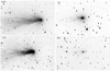 |
Fig. 1 TRAPPIST-South images of comet C/2016 R2 obtained with the CO+, C2, and CN narrowband filters and TRAPPIST-North image obtained with the BC narrowband filter on February 10 and 11, 2018 respectively. The images are oriented with north down and east left. |
Afρ values of comet C/2016 R2.
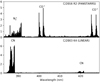 |
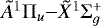
Fig. 2 Comparison of the UVES spectra of C/2016 R2 at 2.8 au and C/2003 K4 at 2.6 au over the 383.0 to 429.0 nm wavelength range. The y-axis has arbitrary units and was chosen independently for both spectra so bright emission features appear with similar intensities. |
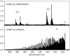 |
Fig. 3 Comparison of the UVES spectra of C/2016 R2 at 2.8 au and C/2003 K4 at 2.6 au over the 476.5 to 519.5 nm wavelength range. The y-axis has arbitrary units and was chosen independently for both spectra so bright emission features appear with similar intensities. |
3.2 Detected and non-detected species
Compared to previous observations of this comet with other high resolution spectrographs at optical wavelengths, UVES spectra have the advantage of covering the whole optical range while having the benefit of being mounted on an 8 m class telescope; this allows us to detect fainter emission bands or species. With this spectrum, we confirm the peculiarity of R2, as illustrated in Figs. 2 and 3, where it is compared to the spectrum of comet C/2003 K4 (LINEAR) obtained with the same instrument and spectral resolution and at comparable heliocentric and geocentric distances (Manfroid et al. 2005). The spectrum of C/2003 K4 is dominated by strong CN emission lines around 390 nm and C2 between 450 and 520 nm, while the spectrum of R2 is dominated by  emission below 392 nm and by CO+ in the 400–620 nm region as already shown by Cochran & McKay (2018). This is also consistent with the CN narrowband images of R2 obtained with TRAPPIST being contaminated by
  emission lines.
The list of species identified in the UVES spectra is given in Table 3, along with their corresponding transitions. The strongest signatures are those of  , CO+, and
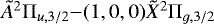
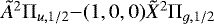
  . In addition to the (4,0), (3,0), (2,0), (4,2), (3,2), (1,0), (2,1), and (1,1) A2Π−X2Σ CO+ bands reported by Cochran & McKay (2018), we detect the (6,0), (7,1), (5,0), (0,0), (0,1), (1,2), and (0,2) bands of the same system. The (0,0), (1,1), and (0,1) bands of the
 first negative group (
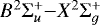 ) are also detected, and we have evidence for the detection of the (0,2) band. Finally, besides
  and CO+, we also detect several
  bands, as illustrated in Fig. 4. In addition to those three ions, which are dominating the spectrum of R2, we detect some of the usual CN, C3, and C2 emission lines, but those are much fainter than in other comets at the same distance (see Fig. 9 for the CN (0,0) band, Fig. 5 for C3, and the very faint C2 bandhead visible in Fig. 3). In Fig. 6, the CH (0,0) band is clearly detected, while it was not in the coma of comet C/2003 K4 (LINEAR) observed at a similar heliocentric distance, indicating that R2 seems to be enriched in CH. We also have a tentative identification of a few CH+ lines.
Species that are usually seen in the coma of similarly bright comets but that could not be detected spectra of R2 are as interesting. We searchedfor OH emission lines to get an indication of the water content of the comet. We looked for matching lines from the A2 Σ+−X2Πi (0,1) band around 345 nm without success. Unfortunately, the setup used did not cover the strongest (0,0) OH emission band around 309 nm. Similarly, we also searched for OH+ lines around 356.5 nm without success. H2O+ has emission lines in the 580–755 nm region, which are regularly detected in the coma of comets (see for example Cochran 2002). Even though, as illustrated in Fig. 7, two faint lines around 618.41 and 619.88 nm (and maybe a third around 614.68 nm) could potentially match the wavelength of H2 O+ emission lines, there is no clear evidence for the detection of H2O+ in the coma of R2.
Ultimately, we looked for NH2 emission lines around 570 nm, which we would have expected in such a bright comet at that distance from the Sun. Those lines were for example easily detected in C/2003 K4 (LINEAR) observed under similar circumstances. In Fig. 8, we show several NH2 lines detected in K4, which are not detected in the coma of R2. Most lines visible in Fig. 8 in the spectrum of R2 belong to the (1,2) CO+ band.
Other observations of R2 at optical or radio wavelengths have been performed. de Val-Borro et al. (2018) measured a CO production rate between 1.09 and 1.44× 1029 mol. s−1 from observations at the Arizona Radio Observatory Submillimeter Telescope during the period January 10–16, 2018. This is consistent with what was measured by Biver et al. (2018) from observations with IRAM on January 23–24, 2018. de Val-Borro et al. (2018) did not detect CH3OH, HCN, CS, H2CO, or HCO+. Wierzchos & Womack (2018) also reported that the comet was depleted in HCN compared to CO. This is consistent with the faintness of the CN (0,0) band in the UVES spectra and TRAPPIST images. Biver et al. (2018) reported the detection of small amounts of HCN as well as the non-detection of OH at radio wavelengths, and confirmed that the comet is strongly depleted in H2 O, CH3OH, H2 CO, HCN, and H2S with respectto CO compared to comets observed at similar heliocentric distances.
From observations performed with the 2.7 m telescope of the McDonald Observatory in December 2017 at optical wavelengths, Cochran & McKay (2018) could not detect CN, C2, C3, or CH, while we see those species about two months later. Although this might be because the comet was further away from the Sun and less active when their observations were done, this is most probably because UVES is mounted on an 8 m telescope, which provides a much higher sensitivity.
Kumar & Shashikiran (2018) reported the detection of H2O+ in the coma of R2 using the LISA spectrograph mounted on the 1.2 m telescope of the Mount Abu InfraRed Observatory (MIRO) from observations performed on January 25, 2018, while we do not convincingly detect H2O+ emission lines two weeks later. However, the spectrum presented by Kumar & Shashikiran (2018) was obtained at much lower spectral resolution. As illustrated in Fig. 7, in the wavelength range of the H2O+ emission lines, we detect numerous emission lines, either belonging to CO+, identified as sky lines, or unidentified. At low resolution, those could be mistaken for H2 O+, so we believe that the detection of H2O+ by Kumar & Shashikiran (2018) should be taken with caution. We also note that H2 O+ is not detected by Cochran & McKay (2018) in their November and December 2017 observations.
Detected species in the coma of comet C/2016 R2.
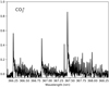 |
Fig. 4 Spectrum of C/2016 R2, showing several |

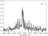 |
Fig. 5 Spectrum of C/2016 R2, showing the C3 (0,0,0)–(0,0,0) |
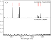 |
Fig. 6 Comparison of the UVES spectra of C/2016 R2 at 2.8 au and C/2003 K4 at 2.6 au over the 429.5 to 432 nm wavelength range, showing the CH lines from the (0,0) band in R2 (indicated by the vertical red lines) and their absence in K4. The y-axis has arbitrary units and has been chosen to display both spectra on a similar scale. |
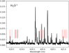 |
Fig. 7 Spectrum of C/2016 R2 showing the region of H2O+ (8,0) band. The red tick marks indicate the wavelength of several of the brightest H2 O+ lines, which are not clearly detected in C/2016 R2. Most lines detected in this wavelength range belong to the CO+ (0,2) band. The y-axis has arbitrary units. |
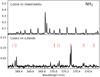 |
Fig. 8 Comparison of the UVES spectra of comets C/2016 R2 at 2.8 au and C/2003 K4 at 2.6 au over the 569.3 to 570.8 nm wavelength range, showing the detection of NH2 lines in K4 (indicated by the vertical red lines, those lines belong to the A(0,10,0)–X(0,0,0) band) and their non-detection in R2. The y-axis has arbitrary units and has been chosen to display both spectra on a similar scale. Most lines detected in R2 in this wavelength range belong to the CO+ (1,2) band. |
3.3 Dust-to-gas ratio
Determining absolute gas production rates from high resolution spectra using a small slit is not straightforward, as a correction for slit losses has to be applied. The CN production rate is particularly difficult to measure in the case of R2 because of the  (0,0) band partly overlapping with the CN (0,0) band. However, using a model of the CN (0,0) band, combined with a Haser profile to determine the part of the flux encompassed in the slit (and scale lengths from A’Hearn et al. 1995), we estimate a CN production rate of (3 ± 1) × 1024 mol. s−1. To perform this measurement, we use the first spectrum obtained on February 11 under clear sky conditions. The CN (0,0) band, along with our best model are shown in Fig. 9.
Using this estimate of the CN production rate and the Afρ measured from TN observations in the BC filter made on the same date, we can compute the Afρ∕Q(CN) ratio, as a proxy of the dust-to-gas ratio of the comet. We obtain a log[Afρ∕Q(CN)] = − 21.78 ± 0.14. Comparing this value to the comets presented in the data set of A’Hearn et al. (1995), and also to more than 30 comets observed with TRAPPIST over the past six years, it is actually higher than for most comets, indicating either a dust-rich or CN-poor comet. We already mentioned previously, and it is illustrated in Fig. 2, that the CN emission in the coma of R2 is faint compared to other comets observed at similar heliocentric distances. Comparing the measured Afρ value to comets observed at similar heliocentric distance by A’Hearn et al. (1995), R2 is within the range of measured Afρ values. Biver et al. (2018) compared the Afρ/CO ratio of R2 to comets at similar distances and with available CO abundances and found it particularly low. The question arises whether R2 is rich in CO or poor in dust. Between 2.5 and 3 au from the Sun, H2 O, CO, and CO2 can all significantly contribute to the comet activity and their relative contributions vary from comet to comet (see for example Ootsubo et al. 2012). A thorough investigation of the dust-to-gas ratio of comets observed at similar distances, accounting for the contribution of the three species would allow us to decipher whether R2 is actually dust poor, or just very rich in CO. However, simultaneous (or close to simultaneous) and reliable measurements of the H2 O, CO, and CO2 abundances in comets observed between 2.5 and 3 au are rare, making such a comparison difficult.
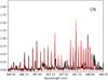 |
Fig. 9 Spectrum of C/2016 R2 showing the CN (0,0) band in black, overlapped with our best CN model (red dashed line). The y-axis has arbitrary units. |
3.4 [NI], [OI] and [CI] forbidden atomic lines
Aside from the molecules mentioned above, we observe emissions from atomic species. The green forbidden oxygen line at 557.73 nm and the red doublet at 630.03 and 636.38 nm are clearly identified (see Fig. 10) and shifted from the corresponding telluric lines owing to the geocentric velocity of the comet. Atomic oxygen in the coma of comets is mainly produced by the photo-dissociation of H2O, CO, and CO2, and, as recently discovered, O2 (Bieler et al. 2015). It has been shown that mixing ratios of CO2∕H2O and CO∕H2O, which are usually very difficult to determine from the ground, can be derived from observations of the ratio of the green oxygen line to the red doublet (G/R ratio) (Festou & Feldman 1981; McKay et al. 2013; Decock et al. 2013, 2015).
For R2, we measure a G/R ratio of 0.23 ± 0.03 on the average spectrum summing all the flux along the slit. Decock et al. (2013) reported a mean value of 0.11 for their sample of 11 comets, which is about twice lower than what we measure for R2. However, both Decock et al. (2013) and McKay et al. (2015) reported that comets observed at larger heliocentric distance have higher values of the G/R ratio. For example, Decock et al. (2013) reported a ratio of 0.3 for comet C/2001 Q4 (NEAT) observed at 3.73 au and ratios of 0.14 and 0.20 for comet C/2009 P1 (Garradd) observed at 2.9 au and 3.25 au, respectively. McKay et al. (2015) measured a ratio of 0.16 for comet C/2009 P1 (Garradd) observed at 2.88 au and McKay et al. (2012) reported a value of 0.24 for comet C/2006 W3 (Christensen) observed at 3.13 au. The G/R ratio measured for R2 is thus consistent with the ratio measured for other comets observed at large heliocentric distances. The increase of the G/R ratio with the heliocentric distance has been interpreted by the fact that the water sublimation becomes less important at distances larger than 2.5 au so that other volatiles such as CO and CO2 start to contribute more significantly to the comet activity. According to Decock et al. (2013), while for comets observed below 2 au the observed mean G/R ratio of 0.09 is consistent with H2O being the main molecule photodissociated to produce oxygen atoms in metastable state, the high G/R ratio measured at large heliocentric distance indicates that at those distances CO and CO2 are contributing. R2 was observed at ~2.8 au from the Sun and its spectrum shows strong emission lines of CO+ and  , while no OH or H2O+ emission lines are convincingly detected. This is consistent with CO and CO2 contributing to drive the activity of R2, implying a higher G/R ratio.
More surprisingly, we detect two lines at 519.79 and 520.03 nm, which we identify as being forbidden nitrogen lines (Wiese et al. 1966), see Fig. 11. To our knowledge, this is the first time those lines are detected in the coma of a comet, even if Singh et al. (1991) mentioned that an unidentified line at 520.1 nm detected in several comets could match the forbidden nitrogen transitions. Those lines are produced by the decay of nitrogen in a metastable state N(2D0). Nitrogen in this metastable state could be produced in the coma of comets by photodissociation of CN for example (Singh et al. 1991). In the Earth atmosphere, nitrogen in the N(2 D0) state is produced by electron impact dissociation of N2, electron impact dissociative ionization of N2, or dissociative electron recombination of  among others (Rees & Romick 1985). Cravens & Green (1978) studied airglow phenomenon in the inner coma of comets and, even though this is not included in their model, they suggested that forbidden nitrogen emission at 520 nm could result from the dissociative excitation of N2. Given the high
  and the low CN abundances in R2, the dissociative electron recombination of
  , electron impact dissociative ionization of N2, and/or the electron impact dissociation of N2 are probably the main contributors to the production of nitrogen atoms in this metastable state. In Fig. 11, we can see that the ratio of the [NI] 519.79 nm to 520.03 nm lines is different for the telluric lines (~2) and cometary lines (~1.2). However, this ratio is expected to vary with the electron density (Dopita et al. 1976) and observations of several planetary nebulae by Aller & Walker (1970) for example showed variations between 0.84 and 1.95. Measurements of the ratio in the Earth atmosphere were performed by Sharpee et al. (2005), which found a mean value of 1.759, close to what we measure for telluric lines.
Forbidden [CI] lines at 872.7, 982.4, and 985.0 nm are emitted from C(1 D), produced by the photodissociation of neutral C-bearing species, electron-impact on the carbon ground-state C(3 P), or dissociative recombination of C-bearingions such as CO+. Even though carbon forbidden lines are regularly detected in the coma of comets at UV wavelengths, the 985.0 nm line was previously claimed to have been detected only once in the coma of comet C/1995 O1 (Hale-Bopp) by Oliversen et al. (2002) using a Fabry-Perot technique. In the spectrum of R2, we first observed a relatively strong line at 985.0 nm and a fainter line at 872.7 nm, as illustrated in Fig. 12 (right and left, respectively), but a priori no emission at 982.4 nm. According to Hibbert et al. (1993), the intensity ratio of the 985.0 to 982.4 nm lines should be about 3, so that we should easily detect the 982.4 nm line. After correction for a strong underlying telluric absorption, using the Molecfit tool (Smette et al. 2015), the 982.4 nm forbidden carbon line is clearly detected (Fig. 12, middle part), though its position, width, and intensity cannot be accurately determined. A more thorough modeling of all forbidden lines and their interpretation in terms of mixing ratio of the main contributors to comet activity is out of the scope of this work and will be done in a subsequent paper.
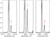 |
Fig. 10 Three forbidden oxygen [OI] lines in comet C/2016 R2 at 557.73 nm (left panel) for the green line, and 630.03 nm (middel panel), and 636.38 nm (right panel) for the red doublet. The cometary oxygen lines are identified by red tick marks, while the dashed blue tick marks indicate the corresponding telluric lines. The y-axis is in arbitrary units. |
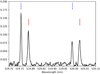 |
Fig. 11 Spectrum of C/2016 R2 between 519.7 and 520.1 nm. The full red tick marks indicate the two cometary nitrogen forbidden lines at 519.79 and 520.03 nm, while the dashed blue tick marks indicate the corresponding telluric lines. The y-axis is in arbitrary units. |
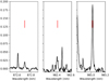 |
Fig. 12 Spectrum of C/2016 R2 corrected from telluric absorption covering the region of the [CI] forbidden lines at 872.7 nm (left panel), 982.4 nm (middle panel), and 985.0 nm (right panel). The red tick marks indicate the position of the carbon forbidden lines. The y-axis is in arbitrary units. |
3.5  abundance ratios
The  , CO+, and
  ions have strong detected emissions, such that we can compute the ratios between those species. For
  , we use the (0,0,0)
 band. Since the majority of the lines identified in that wavelength range are attributed to
  , we measure theband intensity by fitting a continuum on both sides of the band, subtracting it, and then summing the flux over the entire width of the band. As mentioned before, all spectra were subtracted from the dust continuum. The extra continuum subtraction applied removes any residual continuum component that might be left locally. For
  and CO+, we use the (0,0) and (2,0) bands, respectively. Since a non-negligible number of lines not attributed to those species are identified in the wavelength range of the aforementioned bands, we decided to use a different method to measure the intensity of the bands. We first fit and subtract a continuum for each band. In a second time, for each identified line of thosetwo bands, we fit a gaussian and sum all lines of each band. When using the (390 + 580) setting, all three bands of interest are detected in a single setup, allowing us to make the measurements from simultaneous observations.
The  ratio is computed as
![Mathematical equation: \[\frac{{\mathrm N}_2^+}{{\mathrm{CO}}^+} = \frac{g_{{\mathrm{CO}}^+}}{g_{{\mathrm N}_2^+}}\frac{I_{{\mathrm N}_2^+}}{I_{{\mathrm{CO}}^+}},\]](/articles/aa/full_html/2019/04/aa34357-18/aa34357-18-eq43.png)
where  and
and  are the respective intensities of the
  and CO+ bands,
  is the excitation factor of
  from Lutz et al. (1993) (7 × 10⁻² photons s−1 mol.−1), and
  is the excitation factor of CO+ from Magnani & A’Hearn (1986) (3.55 × 10⁻³ photons s−1 mol.−1).
The  ratio is computed as
![Mathematical equation: \[ \mathrm{\frac{CO_2^+}{CO^+}} = \frac{{g}_{\mathrm{CO^+}}}{g_{\mathrm{CO_2^+}}}\frac{I_{\mathrm{CO_2^+}}}{I_{\mathrm{CO^+}}},\]](/articles/aa/full_html/2019/04/aa34357-18/aa34357-18-eq51.png)
where  and
and  are the
  measured band intensity and excitation factor from Kim (1999) (4.958 × 10⁻⁴ photons s−1 mol.−1), respectively. We measure a
  ratio of 0.06 ± 0.01, in very good agreement with Cochran & McKay (2018). Only very low upper limits of 1 × 10⁻⁵ to 1 × 10⁻⁴ for 122P/de Vico, C/1995 O1 (Hale-Bopp), and 153P/Ikeya-Zhang were derived by Cochran et al. (2000); Cochran (2002). Our ratio is higher than the ratio of 0.013 measured for 29P/Schwassmann-Wachmann (Ivanova et al. 2016) but consistent with the ratio of 0.06measured for C/2002 VQ94 (LINEAR) (Korsun et al. 2014).
For the  ratio we obtain a value of 1.1 ± 0.3. Simultaneous measurements of CO+ and
  ions in the coma of comets are scarce. It is then difficult to compare R2 to other comets. Feldman et al. (1997) used the International Ultraviolet Explorer and Hubble Space Telescope observations to constrain the CO2∕CO ratio in several comets. For comets for which both species could be detected, they found ratios ranging between 0.67 and 1.69. For two other comets, they could only derive lower limits of 4.6 and 1.8. However, we cannot infer directly the CO2∕CO ratio in the coma of R2 from the
  ratio. Indeed, CO+ can be produced both from the photoionization of CO and photodissociative ionization of CO2. Few studies comparing the efficiencies of both processes have been performed so far, but Huebner & Giguere (1980) suggested that the photodissociative ionization of CO2 could significantly contribute to the production of CO+ in the coma of comets, especially in the inner coma. The relative contribution of both mechanisms in the coma of R2 is difficult to assess and would require dedicated modeling. Consequently, we must be cautious while interpreting the
  and
and  abundance ratios measured in the coma of this comet.
In their work, as  was not detected Cochran & McKay (2018) considered that the photoionization of CO is the main source of CO+ in order to infer a N2 ∕CO ratio of 0.06 from their measurement of the
  ratio. If we take into account that part of the CO+ detected in the coma of R2 can be produced by the photodissociative ionization of CO2 in addition to the photoionization of CO, the N2∕CO of 0.06 reported by Cochran & McKay (2018) would only be a lower limit.
Since we do not detect H2O+, we attempt to compute an upper limit of the H2O+∕CO+ ratio. We consider the H2O+  (8,0) band, together with the efficiency factor from Lutz et al. (1993) (4.2 × 10⁻³ photons s−1 mol.−1). Since that band is spread over a large wavelength range, over which numerous other emission lines are detected, integrating the flux over the whole wavelength range of the band would not provide a correct upper limit for the H2 O+ flux. Instead, we define zones spanning 0.015 nm on each side of the center of each line of the band in the cometary atlas of Cochran (2002) and integrate the flux over those areas to have a more realistic estimate of the maximum total flux of the H2 O+ band. Using this technique, we measure an upper limit of the H2O+∕CO+ ratio of 0.4. Lutz et al. (1993) reported H2O+∕CO+ ratios varying between 0.6 and 5 for a set of five comets. This is higher than our upper limit for R2, supporting the apparent low water abundance of this comet. However, it is important to keep in mind that the Lutz et al. (1993) measurements have been obtained for comets observed closer to the Sun, where water sublimation is more efficient. Biver et al. (2018) derived an upper limit for the water production rate of R2, leading to an upper limit of the H2 O∕CO ratio of about 0.11. This is consistent with our lowupper limit for the H2O+∕CO+ ratio.
As mentioned earlier, we do not detect NH2 emission lines in the coma of R2. Nevertheless, deriving a lower limit of the  /NH2 ratio would provide an interesting constraint for the solar nebula nitrogen chemistry. We used the NH2 A(0,8,0)–X(0,0,0) band. In the case of R2, the A(0,10,0)–X(0,0,0) band regionshown in Fig. 8 contains a large number of CO+ emissions, making the computation of an upper limit of the NH2 flux difficult. Similarly to what is done for H2O+, we define zones spanning 0.015 nm on each side of the center of each of the brightest lines of the band between 626 and 642 nm and integrated the flux over those areas. We use the fluorescence efficiency from Kawakita & Watanabe (2002) (1.07 × 10⁻³ photons s−1 mol.−1). For all the ratios computed before, we assume an identical dependence of the fluorescence efficiencies with the heliocentric distance as
  . However, in the case of NH2, Kawakita & Watanabe (2002) determined that the fluorescence efficiency actually varies as
  and this is what we used. We then estimate the lower limit of the
  ratio to be about 0.4. It must be pointed out that neutral species and ions have different spatial distributions in the coma and caution must then be taken while interpreting column density ratios between ions and neutral species.
3.6 Nitrogen isotopic ratio
Nitrogen is one of the main species in comets because of numerous molecules containing this atom and detected in their coma (NH3, N2, HCN, NH2CHO, HNCO, HNC, CH3CN, HC3N, C2 H5NO2, CH5N, C2 H7N). So far it has been possible to measure the 14 N/15N ratio from CN and NH2 optical spectra in about 20 comets of various origins. The isotopic ratios measured for these two molecules are in agreement within the error bars: the averaged 14 N/15N ratio from NH2 for 18 comets is 135.7 ± 5.9 (Shinnaka et al. 2016) and this agrees with that in CN for 22 comets, i.e., 145.2 ± 5.6 (Manfroid et al. 2009). This ratio was also measured in HCN (the most obvious parent of CN) for comets 17P/Holmes and C/1995 O1 Hale-Bopp with values of 139 and 205, respectively (Bockelée-Morvan et al. 2008). The 14 N/15N ratio does not seem to vary from one comet to another or with the reservoir of origin. Moreover, long and short period comets present the same ratio (Jehin et al. 2009). It is different from the ratio measured in the Earth’s atmosphere (272 for the N2 molecules according to Nier 1950) or in the presolar nebula (estimated to be 441 from the solar wind, Marty et al. 2011) or 450 from Jupiter’s atmosphere (Fouchet et al. 2004). Bockelée-Morvan et al. (2015) provide a detailed discussion about isotopic ratios. The discovery of R2 presenting numerous N bright emission lines offered a unique opportunity to detect 14 N15N+ emission lines and, consequently, to measure the 14 N/15N isotopic ratio directly in N2, the main reservoir of nitrogen in the solar nebula.
The first step consists in modeling as accurately as possible the N spectrum. The brightest emission lines belong to the (0,0) band of the first negative group, i.e., the
  transition with a bandhead at 391.4 nm. A complete modeling of this spectrum would imply a fluorescence model taking into account all the transitions in this system, with the other bands and, possibly, other electronic transitions, both in absorption (of the solar flux) and in emission. We have not (yet) developed such a model but it is possible to do an acceptable modeling using the Boltzmann distribution(s) with parameters fitted to the observed spectrum.
To model the N spectrum we first compute the energy levels from the constants published by Wood & Dieke (1938) and Lofthus & Krupenie 1977, their Table 72 and the line energies published by Dick et al. (1978). The Einstein coefficients for the spontaneous emission, A
 come from Jain & Sahni (1967) and the Hönl-London factors from Herzberg (1951) (only P and R lines exist for such a transition). From these data and the observed intensities of the cometary emission lines we compute a Boltzmann diagram to see if this spectrum follows a Boltzmann distribution. We find that the relative populations could be satisfactorily fitted by a double Boltzmann distribution based on two different rotational excitation temperatures, Trot ~ 45 K and 860 K; such a two-temperature distribution is not unusual and has been observed for C2 (e.g., see Rousselot et al. 2012; Nelson et al. 2018 and references therein). From these temperatures we manage to fit the observed spectrum in a satisfying manner by adjusting the relative fraction of both populations. Of course such an approximation does not take into account solar absorption lines but, because of the numerous N
 emission lines, the final fit is satisfactory. Fig. 13 presents the result in the range 389–391.6 nm.
The last step consists in computing a similar spectrum for the 14 N15N+ isotopolog emission lines. It is done with the help of the line energies published by Wood & Dieke (1938). Only the emission lines belonging to the R branch are computed since this paper does not contain the P branch data (or only very few) because these emission lines are blended with the bright N emission lines.
To compute the 14 N15N+ emission spectrum we use similar rotational temperatures and ratios between them as fitted on N . Our search for the 14 N15N+ is based on this spectrum. Figure 14 presents the spectrum computed for 14 N/15N = 100 (i.e., an intensity ratio of 50 with the N
 emission lines). As it can be seen no 14 N15N+ emission line is clearly identified. An estimate of the noise in the observational spectrum leads to about 0.02 (arbitrary) intensity units, to be compared to the maximum intensity of the 14 N15N+ synthetic spectrum. Our conclusion is that only a lower limit for the 14 N/15N ratio can be computed. This lower limit is roughly equal to 100.
 |
Fig. 13 Observed (black) and synthetic (red dashed) spectra of the N |

3.7 Dynamical history of R2
We outlined several times that R2 has a very unusual composition, showing strong emission lines of  , CO+, and
  , but no detected water or any of its dissociation product. In order to try to reach a better understanding of the origin of this comet, we decided to have a closer look at its dynamical history.
As we mentioned before, R2 is a nearly-isotropic comet originating from the Oort cloud, belonging to the subclass of returning objects; i.e., it is not the first time that this object has visited the inner region of the solar system (Levison 1996; Dones et al. 2015). According to Fernández (2005), the computation of the original semimajor axis, aorg, and the orbital energy, χorg, is of great interest for long period comets since these parameters are vital to assess the place an object comes from and to determine its dynamical age, i.e., the average number of revolutions it has performed in the inner planetary region. This is particularly interesting in the case of R2, given its peculiar chemical composition.
By definition, the original orbit of a comet is the orbit a comet had before entering the planetary region with respect to the barycenter of the solar system; Fernández (2005) provides further details about the computation of original orbits. R2 has an original reciprocal semimajor axis of 1∕aorg = 0.00129 au−1 (cf. the IAU/MPC Data Base2). From observations and theoretical studies, Fernández (2005) showed that a comet with such a reciprocal semimajor axis (or an equivalent orbital energy of χorg = −0.00129 au−1) performs about ten revolutions before suffering an hyperbolic ejection (χorg > 0). In order to assess the number of revolutions R2 has completed, we decided to study its recent dynamical history through numerical simulations, as it has been done before by other authors for the study of long period comets (see, for example, Hui 2018; Hui et al. 2018, for Jupiter family comets; Pozuelos et al. 2018; Fernández & Sosa 2015, and for activated asteroids; Novaković et al. 2014; and Moreno et al. 2017).
In order to do this study, we use numerical integrations in the heliocentric frame, where the current time is set as the last perihelion passage, i.e., May 9, 2018. We extend our integrations 3 × 10⁵ yr backward. We use the numerical package REBOUND (Rein & Liu 2012), with the integrator algorithm MERCURIUS, which is an hybrid integrator that combines a fast and unbiased symplectic Wisdom-Holman integrator, WHFAST (Rein & Tamayo 2015), and a high accuracy non-symplectic integrator with adaptive time-stepping algorithm that handles close encounters, IAS15 (Rein & Spiegel 2015). Because of the accumulation of errors during the numerical integrations, the dynamical evolution of a long period comet through successive passages by the planetary region is a stochastic process in which in every perihelion passage the comet meets a planetary configuration completely different from the previous one. To solve this, we perform a statistical study in which, in addition to the nominal orbit of the comet, the orbital evolution of a set of clones on orbits corresponding to the uncertainty is also followed. For this purpose, we generate 1000 clones based on the covariance matrix of the orbital elements (Chernitsov et al. 1998).
In order to make the problem tractable with ordinary computational facilities, we split our 1000 clones into 10 sets of 100 clones. The set of orbital elements and the covariance matrix of the orbit of R2 are published together in the NASA/JPL Small-Body browser (JPL 20). The initial timestep is set to five days and the computed orbital evolution is stored every year for each clone. The Sun, the eight planets, and Pluto are included in the simulation. We neglect both Galactic tide and gravitational effects of stars passing close to the Sun; these are the two main effects that contribute to ejecting comets from the Oort cloud to the inner solar system. This assumption is valid because both effects are almost null for objects having semimajor axis well below a ~ 20 000 au (Souchay & Dvorak 2010; Dones et al. 2015). The action of non-gravitational forces might have a significant effect for long period comets approaching the Sun to less than a few tenths of au. However, the evaluation of these forces for long period comets is difficult since they have not been observed in a second apparition during which variations of the time of the perihelion passage could be detected. Thus, for simplicity, we do not include galactic tide, gravitational effects of stars passing close to the Sun, and non-gravitational forces in our simulations.
The orbital evolution of R2 and its 1000 clones in terms of reciprocal semimajor axis, 1∕a, eccentricity, e, and heliocentric distance in the past 1.5 × 10⁵ yr is shown in Fig. 15. Our study shows that in a period between −(50 and 100) kyr 95% of the clones experience a dramatic change in their orbits, suffering hyperbolic ejections, i.e., e > 1 and 1∕a < 0. Therefore, we consider the upper limit of the time during which R2 has been orbiting in its current orbit to be on the order of 150 kyr. Moreover, our simulations show that 72.9% of the clones pass through perihelion only three times, 23.9% pass four times, 2.8% pass five times, and 0.4% pass six times. In all cases, the perihelion distances are in the range 2.6–3.2 au. These results show that R2 is in a dynamical state of evolution within the limits of “young” and “middle-age” as defined in Fernández (2005).
This study indicates that R2 had a relatively quiet recent dynamical history. As a consequence, it does not seem that its peculiar composition is related to its recent orbital evolution. The comet is not at its first passage through the planetary region, so it is not releasing unusual amounts of highly volatile species because it is approaching the Sun for the first time, but it has not been heavily processed due to repeated passages close to the Sun either. This indicates that, while the orbit of R2 is similar to many other Oort Cloud comets, its composition is intrinsically different.
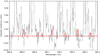 |
Fig. 14 Zoom of the observed spectrum (black) of C/2016 R2 and the 14N15N+ synthetic spectrum computed for 14N/15N = 100 (dashed red curve). The dotted line represents the N |

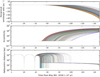 |
Fig. 15 Orbital evolution of C/2016 R2 and 1000 clones over 1.5 × 10⁵ yr backward intime from last perihelion passage on May 9, 2018. Different colors represent different sets of 100 clones (see text for details). From the top to the bottom panels: reciprocal semimajor axis, eccentricity, and heliocentric distance. |
4 Discussion and conclusions
In this work, we present high resolution optical observations of comet C/2016 R2 (PanSTARRS) performed with the UVES instrument at the VLT, complemented by narrowband imaging obtained with the TRAPPIST telescopes. R2 has a very peculiar chemical composition, with strong  , CO+, and
  emission lines in the optical, faint CN, C3, and C2, and no detected OH, OH+, or H2O+, suggesting a comet rich in N2 and CO but relatively poor in water. The comet also has clearly detected CH emissions. Table 4 summarizes the ratios measured in the coma of R2. The non-detection of NH2 seems to suggest that most of the nitrogen content of R2 is concentrated in N2 with a lower limit of the
  ratio of 0.4. Such a high
  ratio might put strong constraints on the origin of R2 through adequate modeling (Womack et al. 1992). In some ways, R2 is similar to comets 29P/Schwassmann-Wachmann and C/2002 VQ94 (LINEAR), which are both distant active comets displaying clear
  and CO+ emission lines.
Because we detect very strong  bands, we attempted to measure the 14 N/15N isotopic ratio from
  directly for the first time. We could derive a lower limit of the 14 N/15N isotopic ratio of about 100, which is consistent with the values measured for comets from CN and NH2 (Manfroid et al. 2009; Shinnaka et al. 2016).
We determine an upper limit of about 0.4 for the H2O+∕CO+ ratio, indicating a low water abundance in the coma of R2. This is in agreement with our measurement of the ratio of the green oxygen forbidden line at 557.73 nm to the red doublet at 630.03 and 636.37 nm. This quantity can be linked to the mixing ratios of CO∕H2O and CO2∕H2O. We measure a G/R ratio of0.23, which is consistent with what has been measured by Decock et al. (2013) for comets observed at large distances from the Sun (>3.0 au), when water sublimation is less efficient and CO and CO2 are significantly contributing to the cometary activity.
For the first time, we clearly detected the [NI] forbidden lines at 519.79 and 520.02 nm in the coma of a comet. These lines are the result of the decay of nitrogen in a metastable state most probably produced in this case by the dissociative electron recombination of  , electron impact dissociative ionization of N2, and/or the electron impact dissociation of N2. We conducted a search in our database of high resolution spectra of a dozen comets observed with UVES over the past 15 years. We do not detect the [NI] lines in any of those comets, among which some have been observed under circumstances similar to those of R2. The unusually high abundance of molecular nitrogen in the coma of R2 might then explain why we detect the [NI] lines in this particular comet and not in others.
The presence of highly volatile species such as N2 or CO in unusually high amounts while other species like water, CN, or NH2 are depleted is difficult to explain. One could wonder whether this comet has undergone only very minor processing since its formation, for example. However, our analysis of its dynamical history shows that R2 is a dynamically middle-aged comet coming from the Oort cloud, having crossed the planetary region at least three times in the past, with perihelion distances of around 2.5–3.0 au. Therefore the peculiar composition of its coma cannot be explained by the fact that it is releasing highly volatile gases far away from the Sun on its first perihelion passage, even though it probably did not undergo strong thermal processing due to a close encounter with the Sun.
Another hypothesis is that the origin of its peculiarity might then be intrinsic and linked to the conditions prevailing in the solar nebula at the time of its formation, to the distance from the Sun, or the time at which it formed. Since we detect significant  emission lines, we cannot derive the N2∕CO ratio from our measurement of the
  . However, we can set a lower limit of 0.06. This value is about ten times higher than that measured in comet 67P, which was interpreted as an indication of a lower limit of 24 K for the temperature experienced by the grains when they agglomerated to form 67P (Rubin et al. 2015). This interpretation is based on the results of laboratory experiments published by Bar-Nun et al. (2007) and their estimation of the N2∕CO depletion factor at three different temperatures (24, 27, and 30 K). For 24 K this depletion factor was found to be ~19, and this value is within the range of that observed in 67P (25.4 ± 8.9). Because this depletion factor increases between 24 K and 27 K, Rubin et al. (2015) considered this work as indicative of a lower limit of 24 K for the temperature experienced by the grains when they agglomerated to form 67P. For R2 we estimate a N2∕CO ratio one order of magnitude above that measured for 67P, with a large amount of N2 and CO, indicating that the temperature experienced by the grains when they agglomerated was lower than 24 K based on the measured efficiency of gas trapping in water ice. It should, nevertheless, be pointed out that different attempts to measure N2 ∕CO from
  with ground-based facilities (Cochran et al. 2000; Cochran 2002) in different comets (153P/Ikeya-Zhang, C/1995 O1 Hale-Bopp and 122P/1995 S1 de Vico) provided upper limits for the N2∕CO ratio to be one order of magnitude lower than the ratio measured in the coma of 67P. An observational bias cannot be excluded because these attempts to measure this ratio are based on a very different observational technique compared tothe in situ ROSINA measurements. These results, nevertheless, seem to indicate that both 67P and R2 are enriched in N2 compared to most comets, the last showing the strongest enrichment in N2. At the end we can only speculate that the temperature of the formation region of R2 was lower than that of 67P, but it is hard to be more accurate on this point.
Alternatively, Biver et al. (2018) suggested that R2 could be a collisional fragment of a Kuiper belt object (KBO). Indeed, some Kuiper belt objects such as Pluto or Eris have N2 -rich surfaces. Large KBOs are differentiated and the radiogenic heating they undergo would release highly volatile gases, which then re-condenses in the outer layers, enriching those layers in volatiles such as N2 or CO. Another clue that could point toward R2 being a KBO fragment is the strong CH emission we detected, which could point to a relatively high methane content. Kuiper belt objects like Pluto and Eris have been shown to have a surface rich in methane. However, even though it is dynamically possible, the likelihood of a KBO fragment ending up on an Oort Cloud orbit should be investigated. In conclusion, more modeling is needed to understand the origin of the peculiar chemical composition of R2 in terms of its place and conditions of formation as well as its evolutionary path.
Ratios measured in the coma of R2.
Acknowledgements
Based on observations made with ESO Telescopes at the La Silla Paranal Observatory under program 2100.C-5035(A). TRAPPIST-South is a project funded by the Belgian Fonds (National) de la Recherche Scientifique (F.R.S.-FNRS) under grant FRFC 2.5.594.09.F. TRAPPIST-North is a project funded by the University of Liège, and performed in collaboration with Cadi Ayyad University of Marrakesh. CO is an ESO fellow. DH, EJ, and MG are FNRS Senior Research Associates. YM acknowledges the support of Erasmus+ International Credit Mobility. FJP is supported by a Marie Curie CO-FUND fellowship, co-founded by the University of Liège and the European Union. We thank Julio Fernandez for his valuable discussion. Simulations in this paper made use of the REBOUND code, which can be downloaded freely at http://github.com/hannorein/rebound. We thank Hanno Rein and Daniel Tamayo for their help using REBOUND. We thank R. Thomas and B. Häußler for performing the observations.
References
- A’Hearn, M. F., Schleicher, D. G., Millis, R. L., Feldman, P. D., & Thompson, D. T. 1984, AJ, 89, 579 [NASA ADS] [CrossRef] [Google Scholar]
- A’Hearn, M. F., Millis, R. C., Schleicher, D. O., Osip, D. J., & Birch, P. V. 1995, Icarus, 118, 223 [NASA ADS] [CrossRef] [Google Scholar]
- Aller, L. H., & Walker, M. F. 1970, ApJ, 161, 917 [NASA ADS] [CrossRef] [Google Scholar]
- Bar-Nun, A., Notesco, G., & Owen, T. 2007, Icarus, 190, 655 [NASA ADS] [CrossRef] [Google Scholar]
- Bieler, A., Altwegg, K., Balsiger, H., et al. 2015, Nature, 526, 678 [Google Scholar]
- Biver, N., Bockelée-Morvan, D., Paubert, G., et al. 2018, A&A, 619, A127 [NASA ADS] [CrossRef] [EDP Sciences] [Google Scholar]
- Bockelée-Morvan, D., Biver, N., Jehin, E., et al. 2008, ApJ, 679, L49 [NASA ADS] [CrossRef] [Google Scholar]
- Bockelée-Morvan, D., Calmonte, U., Charnley, S., et al. 2015, Space Sci. Rev., 197, 47 [NASA ADS] [CrossRef] [Google Scholar]
- Chernitsov, A. M., Baturin, A. P., & Tamarov, V. A. 1998, Solar Syst. Res., 32, 405 [NASA ADS] [Google Scholar]
- Cochran, A. L. 2002, ApJ, 576, L165 [NASA ADS] [CrossRef] [Google Scholar]
- Cochran, A. L., & McKay, A. J. 2018, ApJ, 854, L10 [NASA ADS] [CrossRef] [Google Scholar]
- Cochran, A. L., Cochran, W. D., & Barker, E. S. 2000, Icarus, 146, 583 [Google Scholar]
- Cravens, T. E., & Green, A. E. S. 1978, Icarus, 33, 612 [NASA ADS] [CrossRef] [Google Scholar]
- de La Baume Pluvinel, A., & Baldet, F. 1911, ApJ, 34, 89 [NASA ADS] [CrossRef] [Google Scholar]
- de Val-Borro, M., Milam, S. N., Cordiner, M. A., et al. 2018, ATel, 11254 [Google Scholar]
- Decock, A., Jehin, E., Hutsemékers, D., & Manfroid, J. 2013, A&A, 555, A34 [NASA ADS] [CrossRef] [EDP Sciences] [Google Scholar]
- Decock, A., Jehin, E., Rousselot, P., et al. 2015, A&A, 573, A1 [NASA ADS] [CrossRef] [EDP Sciences] [Google Scholar]
- Dick, K. A., Benesch, W., Crosswhite, H. M., et al. 1978, J. Mol. Spectr., 69, 95 [NASA ADS] [CrossRef] [Google Scholar]
- Dones, L., Brasser, R., Kaib, N., & Rickman, H. 2015, Space Sci. Rev., 197, 191 [NASA ADS] [CrossRef] [Google Scholar]
- Dopita, M. A., Mason, D. J., & Robb, W. D. 1976, ApJ, 207, 102 [NASA ADS] [CrossRef] [Google Scholar]
- Farnham, T. L., Schleicher, D. G., & A’Hearn, M. F. 2000, Icarus, 147, 180 [NASA ADS] [CrossRef] [Google Scholar]
- Feldman, P. D., Festou, M. C., Tozzi, P., & Weaver, H. A. 1997, ApJ, 475, 829 [NASA ADS] [CrossRef] [Google Scholar]
- Fernández, J. A. 2005, Astrophys. Space Sci. Lib. (Dordrecht: Springer), 328 [Google Scholar]
- Fernández, J. A., & Sosa, A. 2015, Planet. Space Sci., 118, 14 [NASA ADS] [CrossRef] [Google Scholar]
- Festou, M., & Feldman, P. D. 1981, A&A, 103, 154 [NASA ADS] [Google Scholar]
- Fouchet, T., Irwin, P. G. J., Parrish, P., et al. 2004, Icarus, 172, 50 [NASA ADS] [CrossRef] [Google Scholar]
- Greenstein, J. L. 1962, ApJ, 136, 688 [NASA ADS] [CrossRef] [Google Scholar]
- Haser, L. 1957, Bull. Soc. R. Sci. Liège, 43, 740 [Google Scholar]
- Herzberg, G. 1951, Am. J. Phys. 19, 390 [NASA ADS] [CrossRef] [Google Scholar]
- Hibbert, A., Biemont, E., Godefroid, M., & Vaeck, N. 1993, A&AS, 99, 179 [NASA ADS] [Google Scholar]
- Huebner, W. F., & Giguere, P. T. 1980, ApJ, 238, 753 [NASA ADS] [CrossRef] [Google Scholar]
- Hui, M.-T. 2018, AJ, 156, 73 [NASA ADS] [CrossRef] [Google Scholar]
- Hui, M.-T., Jewitt, D., & Clark, D. 2018, AJ, 155, 25 [NASA ADS] [CrossRef] [Google Scholar]
- Iro, N., Gautier, D., Hersant, F., Bockelée-Morvan, D., & Lunine, J. I. 2003, Icarus, 161, 511 [NASA ADS] [CrossRef] [Google Scholar]
- Ivanova, O. V., Luk‘yanyk, I. V., Kiselev, N. N., et al. 2016, Planet. Space Sci., 121, 10 [NASA ADS] [CrossRef] [Google Scholar]
- Ivanova, O. V., Picazzio, E., Luk’yanyk, I. V., Cavichia, O., & Andrievsky, S. M. 2018, PASS, 157, 34 [Google Scholar]
- Jain, D. C., & Sahni, R. C. 1967, Int. J. Quant. Chem., 1, 721 [CrossRef] [Google Scholar]
- Jehin, E., Gillon, M., Queloz, D., et al. 2011, The Messenger, 145, 2 [NASA ADS] [Google Scholar]
- Jehin, E., Manfroid, J., Hutsemékers, D., Arpigny, C., & Zucconi, J.-M. 2009, Earth Moon Planets, 105, 167 [NASA ADS] [CrossRef] [Google Scholar]
- Jewitt, D., & Meech, K. J. 1986, ApJ, 310, 937 [NASA ADS] [CrossRef] [Google Scholar]
- Kawakita, H., & Watanabe, J.-I. 2002, ApJ, 572, L177 [NASA ADS] [CrossRef] [Google Scholar]
- Kim, S. J. 1999, Earth Planets Space, 51, 139 [NASA ADS] [CrossRef] [Google Scholar]
- Korsun, P. P., Ivanova, O. V., & Afanasiev, V. L. 2008, Icarus, 198, 465 [NASA ADS] [CrossRef] [Google Scholar]
- Korsun, P. P., Rousselot, P., Kulyk, I. V., Afanasiev, V. L., & Ivanova, O. V. 2014, Icarus, 232, 88 [NASA ADS] [CrossRef] [Google Scholar]
- Kumar, V., & Shashikiran, G. 2018, EPSC Abstr. Eur. Planet. Sci. Congr. 2018, 12 [Google Scholar]
- Levison, H. F. 1996, in Completing the Inventory of the Solar System, eds. T. Rettig, & J. M. Hahn, ASP Conf. Ser. 107, 173 [NASA ADS] [Google Scholar]
- Lofthus, A., & Krupenie, P. H. 1977, J. Phys. Chem. Ref. Data, 6, 113 [NASA ADS] [CrossRef] [Google Scholar]
- Lutz, B. L., Womack, M., & Wagner, R. M. 1993, ApJ, 407, 402 [NASA ADS] [CrossRef] [Google Scholar]
- Magnani, L., & A’Hearn, M. F. 1986, ApJ, 302, 477 [NASA ADS] [CrossRef] [Google Scholar]
- Manfroid, J., Jehin, E., Hutsemékers, D., et al. 2005, A&A, 432, L5 [CrossRef] [EDP Sciences] [Google Scholar]
- Manfroid, J., Jehin, E., Hutsemékers, D., et al. 2009, A&A, 503, 613 [NASA ADS] [CrossRef] [EDP Sciences] [Google Scholar]
- Marty, B., Chaussidon, M., Wiens, R. C., Jurewicz, A. J. G., & Burnett, D. S. 2011, Science, 332, 1533 [NASA ADS] [CrossRef] [Google Scholar]
- McKay, A. J., Chanover, N. J., Morgenthaler, J. P., et al. 2012, Icarus, 220, 277 [NASA ADS] [CrossRef] [Google Scholar]
- McKay, A. J., Chanover, N. J., Morgenthaler, J. P., et al. 2013, Icarus, 222, 684 [NASA ADS] [CrossRef] [Google Scholar]
- McKay, A. J., Cochran, A. L., DiSanti, M. A., et al. 2015, Icarus, 250, 504 [NASA ADS] [CrossRef] [Google Scholar]
- Moreno, F., Pozuelos, F. J., Novaković, B., et al. 2017, ApJ, 837, L3 [Google Scholar]
- Mousis, O., Guilbert-Lepoutre, A., Lunine, J. I., et al. 2012, ApJ, 757, 146 [NASA ADS] [CrossRef] [Google Scholar]
- Nelson, T., Cochran, A. L., & Western, C. 2018, J. Phys. Chem. A, 122, 8020 [CrossRef] [Google Scholar]
- Nier, A. O. 1950, Phys. Rev., 77, 789 [NASA ADS] [CrossRef] [Google Scholar]
- Novaković, B., Hsieh, H. H., Cellino, A., Micheli, M., & Pedani, M. 2014, Icarus, 231, 300 [NASA ADS] [CrossRef] [Google Scholar]
- Oliversen, R. J., Doane, N., Scherb, F., Harris, W. M., & Morgenthaler, J. P. 2002, ApJ, 581, 770 [NASA ADS] [CrossRef] [Google Scholar]
- Ootsubo, T., Kawakita, H., Hamada, S., et al. 2012, ApJ, 752, 15 [NASA ADS] [CrossRef] [Google Scholar]
- Opitom, C., Jehin, E., Manfroid, J., et al. 2015, A&A, 574, A38 [NASA ADS] [CrossRef] [EDP Sciences] [Google Scholar]
- Owen, T., & Bar-Nun, A. 1995, Icarus, 116, 215 [NASA ADS] [CrossRef] [Google Scholar]
- Pozuelos, F. J., Jehin, E., Moulane, Y., et al. 2018, A&A, 615, A154 [NASA ADS] [CrossRef] [EDP Sciences] [Google Scholar]
- Rees, M. H., & Romick, G. J. 1985, J. Geophys. Res., 90, 9871 [NASA ADS] [CrossRef] [Google Scholar]
- Rein, H., & Liu, S.-F. 2012, A&A, 537, A128 [NASA ADS] [CrossRef] [EDP Sciences] [Google Scholar]
- Rein, H., & Spiegel, D. S. 2015, MNRAS, 446, 1424 [NASA ADS] [CrossRef] [Google Scholar]
- Rein, H., & Tamayo, D. 2015, MNRAS, 452, 376 [NASA ADS] [CrossRef] [Google Scholar]
- Rousselot, P., Jehin, E., Manfroid, J., & Hutsemékers, D. 2012, A&A, 545, A24 [NASA ADS] [CrossRef] [EDP Sciences] [Google Scholar]
- Rubin, M., Altwegg, K., Balsiger, H., et al. 2015, Science, 348, 232 [NASA ADS] [CrossRef] [Google Scholar]
- Sharpee, B. D., Slanger, T. G., Cosby, P. C., & Huestis, D. L. 2005, Geophys. Res. Lett., 32, L12106 [NASA ADS] [CrossRef] [Google Scholar]
- Shinnaka, Y., Kawakita, H., Jehin, E., et al. 2016, MNRAS, 462, S195 [CrossRef] [Google Scholar]
- Singh, P. D., D’Ealmeida, A. A., & Huebner, W. F. 1991, Icarus, 90, 74 [NASA ADS] [CrossRef] [Google Scholar]
- Smette, A., Sana, H., Noll, S., et al. 2015, A&A, 576, A77 [NASA ADS] [CrossRef] [EDP Sciences] [Google Scholar]
- Souchay, J., & Dvorak, R. 2010, Dynamics of Small Solar System Bodies and Exoplanets (Berlin, Heidelberg: Springer) [CrossRef] [Google Scholar]
- Weryk, R., & Wainscoat, R. 2016, Central Bureau Electronic Telegrams, 4318 [Google Scholar]
- Wierzchos, K., & Womack, M. 2017, Central Bureau Electronic Telegrams, 4464 [Google Scholar]
- Wierzchos, K., & Womack, M. 2018, AJ, 156, 34 [NASA ADS] [CrossRef] [Google Scholar]
- Wiese, W. L., Smith, M. W., & Glennon, B. M. 1966, Atomic transition probabilities. Hydrogen through Neon. A critical data compilation (Washington, DC: U.S. Government Printing Office) [Google Scholar]
- Womack, M., Wyckoff, S., & Ziurys, L. M. 1992, ApJ, 401, 728 [NASA ADS] [CrossRef] [Google Scholar]
- Wood, R. H., & Dieke, G. 1938, JCP, 6, 734 [Google Scholar]
- Wyckoff, S., & Theobald, J. 1989, Adv. Space Res., 9, 157 [NASA ADS] [CrossRef] [PubMed] [Google Scholar]
All Tables
All Figures
|
Fig. 1 TRAPPIST-South images of comet C/2016 R2 obtained with the CO+, C2, and CN narrowband filters and TRAPPIST-North image obtained with the BC narrowband filter on February 10 and 11, 2018 respectively. The images are oriented with north down and east left. |
| In the text | |
|
Fig. 2 Comparison of the UVES spectra of C/2016 R2 at 2.8 au and C/2003 K4 at 2.6 au over the 383.0 to 429.0 nm wavelength range. The y-axis has arbitrary units and was chosen independently for both spectra so bright emission features appear with similar intensities. |
| In the text | |
|
Fig. 3 Comparison of the UVES spectra of C/2016 R2 at 2.8 au and C/2003 K4 at 2.6 au over the 476.5 to 519.5 nm wavelength range. The y-axis has arbitrary units and was chosen independently for both spectra so bright emission features appear with similar intensities. |
| In the text | |
|
Fig. 4 Spectrum of C/2016 R2, showing several |
| In the text | |
|
Fig. 5 Spectrum of C/2016 R2, showing the C3 (0,0,0)–(0,0,0) |
| In the text | |
|
Fig. 6 Comparison of the UVES spectra of C/2016 R2 at 2.8 au and C/2003 K4 at 2.6 au over the 429.5 to 432 nm wavelength range, showing the CH lines from the (0,0) band in R2 (indicated by the vertical red lines) and their absence in K4. The y-axis has arbitrary units and has been chosen to display both spectra on a similar scale. |
| In the text | |
|
Fig. 7 Spectrum of C/2016 R2 showing the region of H2O+ (8,0) band. The red tick marks indicate the wavelength of several of the brightest H2 O+ lines, which are not clearly detected in C/2016 R2. Most lines detected in this wavelength range belong to the CO+ (0,2) band. The y-axis has arbitrary units. |
| In the text | |
|
Fig. 8 Comparison of the UVES spectra of comets C/2016 R2 at 2.8 au and C/2003 K4 at 2.6 au over the 569.3 to 570.8 nm wavelength range, showing the detection of NH2 lines in K4 (indicated by the vertical red lines, those lines belong to the A(0,10,0)–X(0,0,0) band) and their non-detection in R2. The y-axis has arbitrary units and has been chosen to display both spectra on a similar scale. Most lines detected in R2 in this wavelength range belong to the CO+ (1,2) band. |
| In the text | |
|
Fig. 9 Spectrum of C/2016 R2 showing the CN (0,0) band in black, overlapped with our best CN model (red dashed line). The y-axis has arbitrary units. |
| In the text | |
|
Fig. 10 Three forbidden oxygen [OI] lines in comet C/2016 R2 at 557.73 nm (left panel) for the green line, and 630.03 nm (middel panel), and 636.38 nm (right panel) for the red doublet. The cometary oxygen lines are identified by red tick marks, while the dashed blue tick marks indicate the corresponding telluric lines. The y-axis is in arbitrary units. |
| In the text | |
|
Fig. 11 Spectrum of C/2016 R2 between 519.7 and 520.1 nm. The full red tick marks indicate the two cometary nitrogen forbidden lines at 519.79 and 520.03 nm, while the dashed blue tick marks indicate the corresponding telluric lines. The y-axis is in arbitrary units. |
| In the text | |
|
Fig. 12 Spectrum of C/2016 R2 corrected from telluric absorption covering the region of the [CI] forbidden lines at 872.7 nm (left panel), 982.4 nm (middle panel), and 985.0 nm (right panel). The red tick marks indicate the position of the carbon forbidden lines. The y-axis is in arbitrary units. |
| In the text | |
|
Fig. 13 Observed (black) and synthetic (red dashed) spectra of the N |
| In the text | |
|
Fig. 14 Zoom of the observed spectrum (black) of C/2016 R2 and the 14N15N+ synthetic spectrum computed for 14N/15N = 100 (dashed red curve). The dotted line represents the N |
| In the text | |
|
Fig. 15 Orbital evolution of C/2016 R2 and 1000 clones over 1.5 × 10⁵ yr backward intime from last perihelion passage on May 9, 2018. Different colors represent different sets of 100 clones (see text for details). From the top to the bottom panels: reciprocal semimajor axis, eccentricity, and heliocentric distance. |
| In the text | |
Current usage metrics show cumulative count of Article Views (full-text article views including HTML views, PDF and ePub downloads, according to the available data) and Abstracts Views on Vision4Press platform.
Data correspond to usage on the plateform after 2015. The current usage metrics is available 48-96 hours after online publication and is updated daily on week days.
Initial download of the metrics may take a while.