| Issue |
A&A
Volume 692, December 2024
|
|
|---|---|---|
| Article Number | A1 | |
| Number of page(s) | 12 | |
| Section | Planets, planetary systems, and small bodies | |
| DOI | https://doi.org/10.1051/0004-6361/202450636 | |
| Published online | 28 November 2024 | |
A comparative study of the blue comets C/1908 R1 (Morehouse) and C/2016 R2 (Pan-STARRS)
1
LAM, Laboratoire d’Astrophysique de Marseille, Aix Marseille University,
38 rue Frédéric Joliot-Curie,
Marseille
13013,
France
2
Institut UTINAM UMR 6213 CNRS, Université de Franche-Comté,
OSU THETA, BP 1615,
25010
Besançon Cedex,
France
3
STAR Institute, Université de Liège,
Allée du 6 Août 19c,
4000
Liège,
Belgium
4
Laboratoire Interdisciplinaire Carnot de Bourgogne, UMR 6303 CNRS, Université de Bourgogne,
9 Av. A. Savary, BP 47870,
21078
Dijon Cedex,
France
5
Institut Polytechnique des Sciences Avancées IPSA,
63 bis Boulevard de Brandebourg,
94200
Ivry-sur-Seine,
France
6
IMCCE, Observatoire de Paris, PSL Research University, CNRS UMR 8028, Sorbonne Universités,
UPMC, Univ. Lille 1, 77 avenue Denfert-Rochereau,
75014
Paris,
France
★ Corresponding author; sarah.anderson@lam.fr
Received:
7
May
2024
Accepted:
27
September
2024
Context. The long-period comet C/1908 R1 (Morehouse) is distinguished by its early spectroscopic tail photography, which uncovered notably intense emission bands of N2+ and CO+, similar to the unusual characteristics of the atypical blue comet C/2016 R2 (Pan-STARRS).
Aims. To probe potential parallels with C/2016 R2 further, we revisited the historical spectroscopic plates of C/1908 R1 while leveraging the New Astrometric Reduction of Old Observations (NAROO) project’s advanced sub-micrometric scanner.
Methods. We first reviewed the intensity ratio method, followed by a comprehensive spectroscopic analysis of the original historical plates to determine the comet’s composition. Our analysis also encompassed an evaluation of C/1908 R1’s dynamic trajectory using an N-body integrator and a detailed examination of tail morphology records.
Results. Our findings suggest that C/1908 R1 experienced no significant close encounters as it crossed the inner Solar System, anchoring its origins directly in the Oort Cloud and allowing us to ascertain that this was its inaugural voyage near the Sun. We determined a N2+/CO+ ratio of ~7% along with a dust-poor composition, particularities it shares with C/2016 R2. Moreover, by synthesizing observations of the tail’s structure over the three-month period of visibility, we uncovered a link between tail dislocation events and aurora borealis sightings on Earth. This association underscores the comet tail’s heightened sensitivity to solar wind fluctuations due to its volatile makeup.
Conclusions. The comet C/1908 R1 (Morehouse) emerges as one of the most unaltered relics of our Solar System’s formation, offering another instance of a C/2016 R2-analogous comet. This underscores the importance of preserving and reexamining historical astronomical datasets, not only for historical significance but as a critical resource for contemporary scientific advancement.
Key words: techniques: spectroscopic / celestial mechanics / comets: general / comets: individual: C/1908 R1 (Morehouse) / comets: individual: C/2016 R2 (PanSTARRS)
© The Authors 2024
 Open Access article, published by EDP Sciences, under the terms of the Creative Commons Attribution License (https://creativecommons.org/licenses/by/4.0), which permits unrestricted use, distribution, and reproduction in any medium, provided the original work is properly cited.
This article is published in open access under the Subscribe to Open model. Subscribe to A&A to support open access publication.
1 Introduction
Comets are formed from the agglomeration of icy grains and dust particles leftover from the planetary formation process. Since sublimation only occurs when comets approach the Sun, comets stored at large heliocentric distances have undergone little alteration since their formation and thus represent some of the most pristine relics of the early Solar System. Understanding where each comet originated reveals details of the evolution of the protosolar nebula (PSN) at the time and place the comet formed.
Comets are water-ice rich, with a usual carbon monoxide composition of CO/H2O = 0.2–23% (Bockelée-Morvan & Biver 2017), and are depleted in N2, with a typical N2/CO ratio of 10−4−10−3 (Cochran et al. 2000). This is peculiar, as N2 appears to be abundant in atmospheres and surfaces of the outer Solar System bodies such as Triton or Pluto (Cruikshank et al. 1993; Owen et al. 1993; Quirico et al. 1999; Merlin et al. 2018). The ratio of carbon-to-nitrogen within comets should be similar to that of the Sun, reflecting the PSN’s composition, but comets appear to be nitrogen-deficient by comparison. Owen & Bar-Nun (1995) determined that ices incorporated into comets at around 50K would have N2/CO≈0.06 if N2/CO is ≈1 in the solar nebula. However, rather than being the norm, only a handful of comets have been identified with this anticipated N2/CO ratio in their spectra (Cochran et al. 2000; Anderson et al. 2023), namely C/1908 R1 (Morehouse) (de La Baume Pluvinel & Baldet 1911); C/1940 R2 (Cunningham); C/1947 S1 (Bester); C/1956 R1 (Arend-Roland); C/1957 P1 (Mrkos) (Cochran et al. 2000); C/1961 R1 (Humason) (Greenstein 1962); C/1969 Y1 (Bennett); C/1973 E1 (Kohoutek); C/1975 V1-A (West); C/1986 P1 (Wilson) (Cochran et al. 2000); 1P/Halley (Wyckoff & Theobald 1989; Lutz et al. 1993); C/1987 P1 (Bradfield) (Lutz et al. 1993); 29P/Schwassmann-Wachmann 1 (Korsun et al. 2008; Ivanova et al. 2016, 2018); C/2002 VQ94 (LINEAR) (Korsun et al. 2008, 2014); and potentially C/2001 Q4 (NEAT) (Feldman 2015). The long-period comet C/2016 R2 (Pan-STARRS), hereafter C/2016 R2, stands alone, with a H2O/CO ratio of only 0.32% (Biver et al. 2018; McKay et al. 2019). It had a peculiar abundance of N2+, with N2/CO estimated to be 0.09 (Anderson et al. 2022b), one of the highest ever observed in comets, while its CN composition was relatively low, with a production rate of only (3 ± 1) ×1024 mol/s. In addition, most of the usual cometary species (i.e., radicals, parent molecules, or ionic species) have been detected (OH, CH, C2, C3, CH4, H2CO, CH3OH, HCN, CO2, CO2+, CH+ from Opitom et al. (2019); Biver et al. (2018); McKay et al. 2019). When compared to CO, the abundance ratios of these other species are nevertheless well below their usual values. This comet also presented a dust-poor composition. With A fρ ~ 700 cm (Opitom et al. 2019) and Q(CO) ~1029 molecules/s (Biver et al. 2018; McKay et al. 2019), we got log[A fρ/Q(CO)] = −26.1, which is lower than the average value of log [A fρ/Q(OH)] = −25.4 given by A’Hearn et al. (1995) for a heliocentric distance of 2.6 au. With CO being the dominant species in the coma in that case, it is more representative than OH, which is used for “normal” comets. As a result, this comet was visually blue. This composition, characterized by its high CO and N2+ content along with low water-ice levels and none of the usual neutrals seen in most cometary spectra, makes C/2016 R2 a unique and intriguing specimen, and it is the only comet of its kind known to date.
Comet C/1908 R1 (Morehouse), hereafter C/1908 R1, was a bright (4.8 maximum recorded apparent magnitude; Holetschek 1909) non-periodic comet observed between September and December 1908. At the time, it was spectacular in that its tail presented unexpected and rapid variations in its morphology after having become visible beyond 2au (Chambers 1909). The images were located in the blue, violet, and ultraviolet so that C/1908 R1 was “consequently blue,” and even to the naked eye, it had a “blueish sheen” (Guillaume 1908a) due to ion emission dominating in the coma. The spectrum extended to a considerable height, and the tail was bright enough for a spec-troscopic analysis, which had been performed only once before on the tail of comet C/1907 L2 (Daniel) (Bernard & Deslandres 1908). Unlike for the other comet, the continuous spectrum was notably absent in C/1908 R1 (de La Baume Pluvinel & Baldet 1908), and its coma was depleted in CN (Deslandres 1908; Campbell & Albrecht 1908). Two bright bands at ~4256 Å and ~ 4279 Å (Campbell & Albrecht 1909) were attributed to “other ingredients not recognized” and later proved to be the two branches of the CO+ (2,0) band (de La Baume Pluvinel & Baldet 1911) based on the research of Fowler (1909), who modeled the spectrum in the lab a year after the passage of C/1908 R1. Most remarkably, the line at 3914.7 Å confirmed the strong presence of N2+, which was as abundant in the coma as in the tail (de La Baume Pluvinel & Baldet 1911). This was the first time molecular nitrogen was observed in a comet (Deslandres et al. 1909). With these considerations, we believe that comet C/1908 R1 could potentially be a C/2016 R2-like comet. Understanding its composition and dynamical history could thus reveal precious information regarding the formation of the Solar System.
As comet C/1908 R1 was on a near-parabolic trajectory and not expected to return to the inner Solar System, the only data at our disposal is from observations performed in 1908. Limited technology and observational techniques at that time restrict our understanding of this comet compared to more recent ones. Comprehensive studies on its composition, nucleus size, and dynamics are challenging due to the scarcity ofdata. Fortunately, the quality of the spectroscopic plates prepared during that period combined with the preservation efforts of the Meudon Observatory library archives enables fresh analysis. Leveraging the advanced capabilities of the New Astrometric Reduction of Old Observations (NAROO) project’s high precision sub-micrometric scanner (Robert et al. 2021), we have undertaken a renewed examination of the spectra from comet C/1908 R1 (Morehouse)’s 1908 passage.
We took the opportunity to first employ numerical integration techniques in order to reevaluate the dynamical history of C/1908 R1, which we present in Sect. 2. This is followed by an updated spectroscopic analysis in Sect. 3. In Sect. 4, we reexamine the evolution of the tail’s morphology. Our conclusion draws parallels between the blue comets C/1908 R1 and C/2016 R2, shedding light on their potential implications for understanding Solar System formation.
2 Dynamical history
2.1 Methods
To estimate the dynamical history of C/1908 R1, we selected two independent dynamical models:
Model 1: we simulated the orbit of C/1908 R1 perturbed by the eight planets using MERCURY, a general-purpose software package for carrying out N-body orbital integrations for problems in Solar-System dynamics (Chambers 1999, 2012). We selected its Hybrid integration algorithm. We used the Osculating Orbital Elements on Epoch 2418245.5 (1908-Oct.-31.0) provided by the JPL Small-Body Database (SBD)1. These are shown in Table 1.
Model 2: we simulated the orbit of C/1908 R1 perturbed by the eight planets with REBOUND, a commonly used N-body integrator popular for its simple interface and efficient integrators (Rein & Liu 2012). We selected the high-accuracy non-symplectic integrator with adaptive time stepping (IAS15). REBOUND automatically downloaded the orbital elements of the bodies from the JPL Horizons database (JPL DE 431).
For both models, we generated 1000 massless facsimiles (clones) of C/1908 R1 from the orbital elements (Table 1) and covariance matrix available on the SBD using a multivariate normal distribution with the object’s orbital elements as the mean. If all the trajectories follow the same trend, we can be certain of a comet’s dynamical history; if they diverge, then it is clear we will not be able to retrieve the trajectory. The uncertainties are large due to the limits of precision of astrometric observations at the time as well as the detectability of the comet, limiting the duration of the observation arc.
In both models, we neglected general relativity and the mass of C/1908 R1 when simulating its positions. The non-gravitational forces could not be constrained due to the limited precision of the observations and are not given by the SBD. The positions of the planets and each C/1908 R1 clone were calculated at each time step. The clones are seen as independent test particles and do not interact with each other. For both models, we investigated the dynamical behavior of the comet from 1908 October 31 to 1 Myr in the past.
2.2 Results
Both simulations demonstrate that C/1908 R1 has a clear dynamical past due to a lack of close encounters with the giant planets. The consistency of this result is unexpected, as with an older comet, the uncertainties on the initial orbital conditions are much larger, yet the results clearly converge, as shown for both models in Fig. 1.
For Model 1, only five of the 1000 clones orbited the Sun in the past 1 Myr. None passed <10 au, and only three “originated” <104 au from the Sun. These results are coherent with C/1908 R1 having traveled from the distant Oort cloud ~ 105 au from the Sun. Its heliocentric distance at t = −1 Myr is on average (8.6 ± 2.8) × 104 au for Model 1 (Fig. 2). At this distance, galactic tidal forces would dominate, placing the object in the interstellar regime. The average eccentricity at t = −1 Myr is 1.16 (Fig. 2). With 88% of the clones having a hyperbolic orbit combined with a semi-major axis >104 au, this comet is an Oort cloud object and dynamically new. For Model 2, the average eccentricity at t = −1 Myr is one, and the average distance is 7.3 ×10⁴ au, similar to the results of Model 1. Only 30 passages under <10 au were recorded across all 1000 clones. However, the final clones are more dispersed: 80% of all the clones have e > 1, compared to 88%. This is likely due to the non-identical batches of clones, which were generated independently. Since there were no close encounters with Jupiter, the integrators computed both evolutions the same way; thus, the results should be viewed together as a 2000-clone evolution.
The high eccentricity of 1.16 for Model 1 and 1.0 for Model 2 at t = −1 Myr alone is not enough to determine if the comet is interstellar, so we had to calculate the excess velocity. Its value is based on the conservation of orbital energy:

Using the orbital elements obtained from the SBD, the estimated v∞ for this comet is 0.9 km/s. This value is significantly lower than the excess velocities of interstellar objects 1I/’Oumuamua and 2I/Borisov, which are 27 km/s and 33 km/s, respectively. The comparatively lower v∞ of C/1908 R1 suggests that it is more likely to have originated within the Solar System rather than interstellar space. With a perihelion distance of less than 1 au and considering a velocity on the order of the Solar System velocity in the local standard of rest (LSR) of ~20 km/s for v∞, this implies that an eccentricity of around 1.43 would be necessary for C/1908 R1 to have arrived from beyond the Solar System. Considering a possible lower estimate for the Solar System velocity of 13.4 km/s in the LSR (Ayari & Elsanhoury 2024), an eccentricity of 1.19 would suffice for C/1908 R1 to have been interstellar. When using the Gaia Collaboration (2021) value for the Solar System velocity of 14.6 km/s in the LSR, we would have a more conservative value of 1.23. As a point of comparison, interstellar object 1I/’Oumuamua had an eccentricity of 1.20113 ± 0.00002 (SBD). This suggests that C/1908 R1 was still loosely bound to our Solar System despite its hyperbolic inbound trajectory. The comet appears to be dynamically new and is likely on its first passage of C/1908 R1 back into the inner Solar System since it was placed in the Oort cloud billions of years ago. As a result, C/1908 R1 may be one of the most pristine remnants of our early Solar System found to date. However, we must accept the fact that, due to the nature of the galactic tides, we do not know if it once completed a similar orbit an extremely long time ago. Nevertheless, such an orbit is unlikely, as the odds of an Oort Cloud object making two independent trips to the inner Solar System are infinitesimally small, as the galactic tides are more likely to reduce the perihelion distance of comets (Fouchard et al. 2006). In any case, C/1908 R1 was clearly stored at the outer edge of the Oort Cloud, though further knowledge of the galactic tides must be evaluated in order to determine how stable its position truly was.
Osculating orbital elements of C/1908 R1 and C/2016 R2 used during our dynamical study.
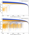 |
Fig. 1 Dynamical history of comet C/1908 R1 Morehouse (black) as estimated with 1000 clones from Model 1 using the MERCURY integrator (above, as presented in Anderson et al. 2023) and Model 2 using the REBOUND integrator (below). Clones with e < 1 at the end of the 1 Myr are shown in orange, and those with e > 1 are shown in blue. All clones reached the end of the 1 Myr integration. |
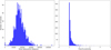 |
Fig. 2 Distribution of the final heliocentric distance (left) and eccentricities (right) of comet C/1908 R1’s clones from Model 1 at the end of the −1 Myr simulation. The average eccentricity is 1.16 ± 0.27, with a median value of 1.07, meaning this comet likely had a hyperbolic orbit. The average heliocentric distance is (8.6 ±2.8) × 104 au. |
2.3 Comparison with C/2016 R2
To determine if the comets C/1908 R1 and C/2016 R2 had similar dynamical origins, we revisited the dynamical simulations conducted on the latter in Anderson et al. (2023) using the same models and methods. We generated 1000 massless clones of C/2016 R2 from the orbital covariance matrix. Using both MERCURY (Model 1) and REBOUND (Model 2), we calculated the positions of the planets and each clone at each time step, neglecting general relativity and the mass of the clones. More details can be found in the 2023 paper.
Both models show all the clones sharing the same trajectory for a single orbit, approximately 19,000 years. C/2016 R2 then undergoes a close encounter with the giant planets, with clones passing on average within 2 au of Jupiter. This encounter introduces significant uncertainties in the comet’s past trajectory due to the scattering effect. Beyond this encounter, the comet’s behavior is chaotic, and its final orbit depends entirely on its last interaction with a giant planet. We cannot quantify when this last interaction occurred, as each successive interaction erases the memory of the previous one. Therefore, it is impossible to determine the precise trajectory of a comet with close encounters in its dynamical past. Our knowledge of C/2016 R2’s past is reliable only for this 19 000-year window. Given that volatiles would not have survived multiple passes near the Sun since the formation of the Solar System, it is likely that C/2016 R2 was once an Oort Cloud object deviated by Jupiter during its visit to the inner Solar System, making it dynamically old in any case, unlike C/1908 R1.
3 Estimating the N2/CO ratio in C/1908 R1
3.1 Intensity ratios
The detection of molecular nitrogen (N2) in comets has posed significant challenges due to its lack of permanent dipole moment, which makes pure rotational transitions invisible at millimeter wavelengths. However, we can indirectly identify N2 in comets from ground-based observations by searching for its daughter ion, N2+, which emits detectable optical signals in the first negative group  bands, with the (0,0) bandhead occurring at 3914 Å. By measuring the intensity of N2+ bands in the comet’s spectra and assuming solar resonance fluorescence as the main excitation source, it is possible to derive ionic ratios of N2+/CO+ in the coma. As both molecules have similar photoionization rates (Huebner et al. 1992), CO and N2 should then be ionized in proportion to the number of neutrals and N2/CO ~ N2+/CO+ in the coma. This method was used to make the first estimates of N2/CO in C/2016 R2 (Cochran & McKay 2018; Opitom et al. 2019).
We applied a similar approach to estimate the quantity of N2+ present in the coma of C/1908 R1. We examined the given band intensities of the observed N2+ in its spectra. Since the column density of a species is given as
 (1)
(1)
where N is the column density, Iv′v″ is the integrated band intensity, and gv′v″ is the excitation factor, we determined the ratio of the column density for these two species to be
 (2)
(2)
We took defined intensities from the literature on C/1908 R1, with the intensities in arbitrary units. Swings & Page (1950) recalculated the intensities in 1950 when estimating the values of comet C/1947 S1 (Bester), basing their values on the research of Baldet (1926), who averaged all 28 plates (72 hours and 49 minutes) of the de La Baume Pluvinel & Baldet (1908) observations. The first estimated intensities of CO+(2,0) by Deslandres et al. (1909) and Campbell & Albrecht (1908) are too high, as the transition at 4273 Å is contaminated by the N2+ (0,1) group, but this is corrected for in Swings & Page (1950). We used the ɡ factors of ɡCO+ = 1.47 × 10⁻¹⁴ erg s−1 ion−1, computed from the Rousselot et al. (2024) model for an heliocentric velocity of −20 km s−1 (close to the average heliocentric velocity during the period of observations), and  erg s−1 ion−1 (Rousselot et al. 2022) along with Eq. (2). We found that N2+/CO+ is between about 0.007 and 0.04. These values and the subsequent results are shown in Table 2.
The results point to a higher than usual N2/CO ratio. The value estimated with the intensities given by Swings & Page (1950) is more reasonable, as they removed the N2+ contamination and are more aware of the complications regarding the spectroscopy of the era. These values were later reestimated by Cochran et al. (2000), who found a N2/CO ratio of 0.06. These values were given through personal communication with C. Arpigny, and the methodology is not detailed in their study, though they took extreme care to avoid the N2+ telluric lines. Overall, the intensity ratios from the literature do not give a clear picture of this comet’s N2/CO ratio, demonstrating the need for a reanalysis of the original plates.
Measured intensities and resulting N2+/CO+ ratios for C/1908 R1 estimated from the literature.
3.2 Spectroscopic analysis
3.2.1 Observational data and scans
We have access to a collection of valuable photographic plates that provide crucial insights into the comet observations of the early 20th century. This collection has provided us with a comprehensive set of 24 plates covering the dates from 16 October to 29 November 1908. Twenty of the plates are of the comet, and four are of reference stars. All are meticulously conserved in the Meudon Observatory library2. Among these plates are spectra taken by A. de la Baume Pluvinel in collaboration with F. Baldet at the Juvisy Observatory (de La Baume Pluvinel & Baldet 1908, 1911). The plates from 29, 30, and 31 October and 1 November bear annotations indicating the positioning of prisms and the use of a spectrograph with objective prism and quartz. Furthermore, we have access to spectra obtained at the Meudon Observatory by A. Bernard and H. Deslandres, whose observations began on 14 October 1908 (Deslandres 1908; Deslandres et al. 1909). Access was also granted to A. Bernard’s notebook, offering further insight into the observational techniques and equipment used during this period.
We employed the NAROO digitization center to digitize the plates, utilizing its high-precision sub-micrometric scanner tailored for the analysis of astrophotographic plates and the examination of historical astronomical data. The scans produced high-quality FITS files.
3.2.2 Extraction and processing of plate spectra
We extracted spectra from the plates, calibrating them in wavelength through the use of comet or reference star lines and by conducting relative flux calibration with the standard stars δ Cygni and Capella. We also had as reference the spectra of Vega taken on 13 and 29 October 1908 and a spectrum of Capella taken on 19 January 1909 (de La Baume Pluvinel & Baldet 1911). For some of these nights, the projection of the reference star’s spectrum is directly on the plate. To accomplish this, the original observers meticulously aligned the comet’s nucleus with a significantly large crosshair during the exposure. At the exposure’s conclusion, the comparison star was positioned on this same crosshair and adjusted according to diurnal motion. This method, while less precise than conventional slit spectrographs due to the large crosshair and manual adjustments, was reported to yield consistent measurements across both small and large prisms (Deslandres 1908). It is also important to note the potential underestimation of atmospheric extinction, which could arise from the differing positions of the stars (generally higher than the comet) and the unknown non-linear response of the photographic plate.
Ultimately, only four dates yielded data of sufficient quality (the rest were deemed too poor for use): 18,30, and 31 (combined with November 1 by the observers; de La Baume Pluvinel & Baldet 1911) October 1908 and 28 November 1908. The details of the plates are listed in Table 3.
Plate 1 contains data from 18 October 1908 (de La Baume Pluvinel & Baldet 1908, 1911). It shows saturation at the center of the bands, and the star’s spectrum is completely saturated. As a result, caution must be exercised when interpreting these results, especially regarding line ratios due to the saturation. It is necessary to determine if these results significantly deviate from other spectra. For this spectrum, wavelength calibration was performed using comet lines. Due to the saturation of the star, flux calibration was not conducted for this spectrum. The airmass was 1.03–1.82.
Plate 2 contains data for 30 October 1908 (Deslandres 1908). We extracted the comet spectrum on 28 pixels from the head in the direction of the tail and conducted relative flux calibration using δ Cygni, which is projected on the plate. A scan of this plate is presented in Fig. 3.
Plate 3 has data from 31 October to 1 November 1908 (de La Baume Pluvinel & Baldet 1908, 1911). Two spectra were extracted corresponding to the positions of the nucleus extracted over 25 arcmin and the tail between 36 and 74 arcmin from the nucleus. Due to the numerous stars in the field, tail spectra could not be indiscriminately taken. The standard star used was Capella, but we were not able to find spectrophotometric data for this star. Consequently, we used a flux-calibrated star with a similar spectral type to Capella (G3III). The star HD 199951, with a B-V=0.88, was selected, as it is closer to Capella’s B-V of 0.80, compared to the Sun’s 0.65. Upon comparison with Capella’s spectrum, the wavelength calibration appears accurate up to 3580 Å. Below this threshold, identification becomes challenging, though a CO+ band (and possibly NH) can still be discerned. Figure 3 represents the scan of this plate. The airmass was 1.20–1.58.
Plate 4 has data from 28 November 1908 (Deslandres 1908). This spectrum was calibrated under the assumption that the star in question is indeed Vega. Though we couldn’t find any definitive information, it is clearly a hot star. The comet was located in the Scutum constellation but was very low on the horizon, explaining the relatively short exposure time. Altair, being closer, might also have served as a reference. We made an extraction around the nucleus.
Spectroscopic plates and resulting N2/CO ratios when this ratio can be computed.
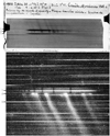 |
Fig. 3 Two of the spectroscopic plates scanned from the Meudon Observatory library archives. Top: scan of Plate 3 obtained over two combined nights 31 October and 1 November 1908 (de La Baume Pluvinel & Baldet 1908, 1911). This spectrum (2-, indicating the nucleus region) was obtained at the Meudon observatory. As the prism objective used to take the spectra has no slit, all the objects in the field of view are dispersed. The spatial extension of the comet ion tail is visible for each of the bright CO+ bands. There is no obvious continuum visible on the head of the comet. The text translates to “1908 October 31 6h12 to 11h10, November 1 6h27 to 8h30. Length 7h01. Comet Morehouse 1908c. Objective prism of spar and quartz – violet light plate – comparison star: Capella.” The two bright spectra correspond to the Capella spectrum, used as a reference star for relative flux calibration. Bottom: Scan of Plate 2 from 30 October 1908 (Deslandres 1908). This spectrum (2-, indicating the nucleus region) was obtained at the Meudon observatory using a 24 cm refractor telescope equipped with an objective prism. The bright spectra correspond to the spectrum of δ Cygni (1-), which is used as a reference star for relative flux calibration. The long horizontal streaks (i.e., 3-) are field stars dispersed and not tracked by the telescope. |
3.2.3 Analysis
Our detailed spectral analysis of comet C/1908 R1 revealed distinct emission bands of N2+ and CO+, allowing us to precisely determine the N2+/CO+ ratio. To model the blue part of the spectrum, where these emission bands are located, we used fluorescence models developed for N2+ (Rousselot et al. 2022) and CO+ (Rousselot et al. 2024). After conducting several tests, we determined an FWHM of 16 Å for the Gaussian instrument response function to be optimal for convolving the theoretical spectrum. The spectral absorption lines of Vega, used as a reference, are well defined and sharp, confirming the resolution of our setup. The wings of this profile are largely obscured by noise, justifying the chosen Gaussian approximation for simplicity. For the CN emission band near 3880 Å, we used a high-resolution spectrum obtained for a similar heliocentric velocity (−19 km s−1) on comet C/2000 WM1 (LINEAR) in June 2000 with the Ultraviolet-Visual Echelle Spectrograph (UVES) mounted on the ESO 8.2-m UT2 telescope of the Very Large Telescope (VLT) with a spectral resolution of about 0.06 Å (the first spectra obtained with UVES; Arpigny et al. 2003). We adjusted the background and subtracted a (small) solar continuum before modeling the spectra.
For plate 1 (18 October 1908), the lack of reference star relative flux calibration prevented us from doing any realistic modeling of these data. We chose not to take this plate into account.
For plate 2 (30 October 1908), we conducted 15 different spectral slices along the comet’s tail moving away from the head and covering a total of 28 pixels. We proceeded to average this value and conduct a fit with a similar spectral resolution (16 Å) by using a N2+/CO+=7.9 %. This fit can be seen in Fig. 4.
For plate 3 (31 October–1 November 1908), we first examined the nucleus region, where the signal-to-noise is the best. Emission bands due to CO+ – mainly (4,0) band around 3800 Å and (3,0) band around 4000 Å − and a blend of CN (0,0) and N2+ (0,0)+(1,1) bands around 3900 Å − plus a faint (5,1) CO+ band – are clearly visible. We managed to get a satisfactory fit of this region by adjusting the relative intensities of these different species. The presence of a weak C3 emission band near 4050 Å is also possible. Our modeling is based on a N2+/CO+ ratio of 7.7%. The uncertainty on this value, related both to the flux calibration and the limit of our modeling, should be of the order of about 2%. Figure 4 presents the result of this modeling. We also tried to fit the spectrum extracted in the tail, which has a lower signal-to-noise ratio. The result appears in Fig. 4 and is based on a N2+/CO+ ratio equal to 6.2%. The uncertainty on this ratio is nevertheless larger. This tail spectrum does not seem to reveal any significant change in the CN band intensity compared to the N2+ and CO+ bands, but once again, the poor signal-to-noise ratio prevented us from being more precise about this relative intensity.
For plate 4 (28 November 1908), we also managed to get a satisfactory fit of the observational spectrum despite a smaller signal-to-noise ratio, especially in the blue part. For this night, we used only the spectra obtained on the nucleus. Figure 4 presents the results of this modeling. It is based on a N2+/CO+ ratio of 7.2%.
Leveraging a century’s worth of laboratory spectra, we revisited the “radiations not identified” as described in de La Baume Pluvinel & Baldet (1911). The lines they highlight at 3932 Å, 3949 Å and 3969 Å and between 4023 Å and 4067 Å might be due to C3 emissions (Cochran & Cochran 2002), though there is no obvious C3 band at 4050 Å, making it impossible to conclusively attribute these lines to C3 without further supporting evidence. This compound was not formally identified at the time due to the limitations of early 20th century spectroscopic techniques.
To search for water, we also looked to the red part of the spectrum in order to identify the H2O+ bands, which are very often present in bright comets at perihelion around 1.0 au, but we could not identify the usual brightest bands at 620 and 590 nm. In Table VI from Baldet (1926), a non-identified band is reported at 7027 Å that corresponds very well to the H2O+ (0,6,0) band, but this region is also very rich in NH2, which is brighter on the comet optocenter. The original observers specified it was found in the head of the comet, which favors the NH2 identification. This is in addition to the fact that two other non-identified bands at 5369 Å and 4987 Å also correspond to NH2-rich regions. In 1926, NH2 was not yet identified in comets. We would also expect to see bright H2O+ (0–8–0) bands at 6183−6216 Å, but these are not noted in their table.
We have no measurements of OH, as the spectrum does not go so far into the blue (so there is no estimation of H2O), and no direct measurement of A fρ due to the lack of absolute flux calibration of the spectra, as the exposure time of the reference stars was not given. While we were able to find the exposure time for one of the plates, it is unfortunately on the order of a minute compared to the hour-long exposures for the comet. Without knowledge of the plate’s reciprocity, this reference cannot be used for reliable calibration. Based on estimates, C/1908 R1 had an approximate magnitude of five around 30 October (Holetschek 1909). For comparison, comet C/2012 K1, which had similar heliocentric and geocentric distances in October 2014 (1.30 au and 1.12 au, respectively), was recorded with a visual magnitude of approximately 7.5 according to Seiichi Yoshida’s website3. The TRAPPIST measurements for C/2012 K1 give an A fρ value of roughly 4 × 103 cm (Jehin et al. 2011). By extrapolation, C/1908 R1 A fρ could be around 4 × 104 cm, assuming comparable magnitudes and contributions from dust and gas emissions. This is typical for bright comets near the Sun. However, C/2012 K1 may not be the best comparison to C/1908 R1, for which the total magnitude may have been less representative of a dust coma and instead more of a CO+-dominated one. An A fρ of 104 cm may be an upper limit. For comparison, C/2016 R2 had an A fρ of only ~750 cm at 2.8 au, indicating a dust-poor composition (Opitom et al. 2019). The observed solar continuum was described as weak for C/1908 R1, but due to the lack of exposure time given for the comparison stars, we were unable to determine the absolute flux and assign a value. This also prevented us from quantifying the CN production rate from C/1908 R1’s spectrum. However, a weak solar continuum is a trait also observed in C/2016 R2, likely due to a low dust content, as it is not sufficient to scatter the visible-UV part of the continuous spectrum.
In this case, we assumed C/1908 R1 is neither dust-poor nor H2O-poor so that we could use the relation determined by Jorda et al. (1991):
![$\log Q\left[ {{{\rm{H}}_2}{\rm{O}}} \right] = 30.76 - 0.25{m_H},$](/articles/aa/full_html/2024/12/aa50636-24/aa50636-24-eq8.png) (3)
(3)
where mH 5.04 is the heliocentric magnitude of the comet (corrected from the distance to the Earth) and Q[H2O] is the water production rate. We found a log Q[H2O] of 29.5 molec/s, indicating an active comet, though not exceptionally so. However, this assumes the comet has a typical composition, which is unlikely to be the case for C/1908 R1. What complicates the comparison is a possible bias in water production for C/2016 R2 due to its large heliocentric distance, with its perihelion at 2.7 au, when the sublimation efficiency of H2O is less than at 1.1–1.4 au; C/1908 R1 has a perihelion of 0.9 au.
Taken together, the shared traits (i.e., the high N2/CO ratio and the weak solar continuum scattered by a low dust production) between C/1908 R1 and C/2016 R2 underscore a remarkable compositional kinship, hinting at a rare comet type with unique evolutionary histories and physical properties. These similarities indicate that both comets may belong to a distinct compositional group that diverges from typical cometary profiles. The definitive absence of water would be the clearest evidence for this shared composition, supporting the classification of C/1908 R1 and C/2016 R2 into a new category. However, with this this aspect still being unknown, such categorization remains an open question.
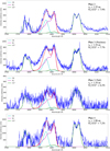 |
Fig. 4 Observational spectrum (blue), after the subtraction of a (very small) solar continuum with the overall fit (red), the sum of CO+ (green), |

4 Morphology of the tail
Given C/1908 R1’s bright nature and circumpolar position (see Fig. 5), the comet attracted attention from both professional and amateur astronomers, enabling continuous observation due to its visibility throughout the night. Its proximity to Earth, sometimes less than 1 au, further facilitated detailed examination. The rise of widely accessible photographic techniques coincided with the comet’s appearance, leading to an extensive collection of visual records preserved on photographic plates. These records have been critical for studying the comet’s composition and morphology. Notable are the rapid changes described in C/1908 R1’s visual morphology. Eddington (1909) highlighted that half-hour exposures blurred the details, suggesting exposures of no longer than ten to fifteen minutes.
The most remarkable trait of this comet was its ever-changing tail. C/1908 R1 underwent a cycle of tail brightening and loss followed by the ejection of a “mass” or “condensation” composed of N2+ and CO+ (De la Baume Pluvinel & Bladet 1912), which was described on multiple occasions. An example of this on the night of 30 September to 1 October 1908 can be seen in Fig. 6. These events can be attributed to various phenomena: rapid sublimation events producing strong gas jets, interactions between the solar wind and the comet’s ions, and magnetic influences such as kink instabilities or tail disconnection events (TDE), though determining which phenomenon is behind the behavior of the tail is difficult due to the limitations of the observations. After a careful review of the literature (see Table 4), we found that the average time between the events is approximately 15 days. While this could be linked to the rotation of C/1908 R1’s nucleus, this should be on the order of a few hours, not weeks. The loss of tail events from the comet may be attributed to strong solar wind disturbances or coronal mass ejections (CMEs) emanating from the Sun. As noted by Griffin (1909), there is a potential correlation between the comet’s remarkable transformation on the night of 30 September and the “vivid display” of the aurora borealis witnessed across the northern United States on the preceding evening, 29 September (Sidgreaves 1908). Notably, 1908 marked a period close to a solar maximum, during solar cycle 14. Given the relative positions of the comet and Earth during this occurrence (see Fig. 5), Earth would likely experience the effects of a CME about 30 hours before the comet did. We found that aurora borealis were also observed on other nights preceding the TDEs (see Table 4). It would thus seem possible that the activity of comet C/1908 R1’s tail was directly linked to the solar activity at the time. Unfortunately, the lack of specific times for the TDEs and auroral events makes it impossible to determine anything more about these events beyond their shared correlation to solar activity.
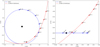 |
Fig. 5 Relative positions of the Earth (blue) and comet C/1908 R1 Morehouse (red) during its 1908 passage (JPL Horizons). The black disk represents the position of the Sun. |
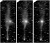 |
Fig. 6 Photographs of the disconnection event in the tail of comet C/1908 R1 from the night of 30 September–1 October 1908 by August Kopff at 20h19 (left), 22h39 (middle), and 00h59 (right). The digitized glass plate archives were made available by the Heidelberg-Konigstuhl Observatory in Germany. |
5 Discussion
The question remains as to what exactly comets C/1908 R1 and C/2016 R2 are. Mousis et al. (2021) and Price et al. (2021) argue that the peculiar composition of C/2016 R2 could reflect formation in specific regions of the solar nebula, particularly near the N2 and CO icelines. Our research in Anderson et al. (2022a) showed that objects formed near the N2 and CO icelines could have been ejected during a phase of dynamical instability in the protoplanetary disk, allowing the comets to preserve their protosolar N2/CO. Schneeberger et al. (2023) further supports this view by showing that icelines can lead to peaks of volatile abundance that are water-depleted, although the observed N2/CO ratios in their study were lower than those for C/2016 R2. However, this is model-dependent, and our understanding of the locations of these icelines is still limited.
Another hypothesis is that these comets are fragments of a differentiated object (Biver et al. 2018; Desch & Jackson 2021; Jackson & Desch 2021). This is supported by De Sanctis et al. (2001), who noted that CO and other volatiles could be nearly absent in the upper layers of differentiated comets, suggesting that C/2016 R2 and possibly 2I/Borisov could be fragments from the cores of such objects. Desch & Jackson (2021) proposed that C/2016 R2 might be a nitrogen iceberg, a fragment from a differentiated KBO’s surface (similar in composition to Pluto) created during the Solar System’s early dynamical instability. Augé et al. (2016) find that the irradiation of N2-CH4 rich surfaces of icy bodies leads to the formation of poly-HCN-like residue, which may be worth looking for. Future studies will need to assess the feasibility of forming these differentiated objects, whether a N2- and CO-rich water-poor composition would be more likely in a surface or a core, the likelihood of their collisional fragmentation, and the mechanisms that could transport these fragments to the Oort Cloud or eject them from the Solar System.
The only other recorded “blue comet” is C/1961 R1 (Huma-son) (Greenstein 1962; Biver et al. 2018). It shares many similarities with C/1908 R1 and C/2016 R2, presenting a bright and defined coma already at a large heliocentric distance (r ~ 2.6 au, a similar distance to which C/2016 R2 was observed). C/1961 R1 exhibited exceptionally intense activity, with a rapid variation of its brightness. With a visual magnitude of 3.5, the radius of its nucleus was estimated as being between 30 and 41 km, making it a massive comet (Öpik 1964, 1963). It had an unusually disrupted, or “turbulent,” appearance (Brandt & Chapman 2004), and at one point between two observations in July 1962, the tail broke off the nucleus (van Biesbroeck 1962). It also presented a strong CO+ and N2+ emission with a “tremendously active” tail (Swings 1965) and weak emission in the continuum. CN, CO2+, and C3 were present but weaker than expected, with only a “trace” of CH+ (Greenstein 1962). Usually CO+ is observed only in the tail, but here it was detected even in the coma (Warner & Harding 1963). This event also represents the first time CO+ was seen in a comet’s tail with such a high resolution. N2+ was found to be strong, while  was weak (Greenstein 1962). In Anderson et al. (2023), we reestimated its N2+/CO+ to be 0.028–0.043. If the spectroscopic plates are still preserved, this comet presents an opportunity to examine another one of these rare blue comets, perhaps giving us another attempt at determining the H2O/CO ratio.
Comparison of Comet C/1908 R1 tail observations and auroral sightings between September and December 1908.
6 Conclusions
Comet C/1908 R1 (Morehouse) exhibits a clear dynamical history with no close encounters with the giant planets, indicating its status as a dynamically new object. The results of our dynamical models converge despite the larger uncertainties on the initial orbital conditions from older observational instruments. The preservation of the pristine state of C/1908 R1 makes it a valuable relic from the early Solar System. C/1908 R1’s position at the outer edge of the Oort Cloud highlights the need for further investigation into the effects of galactic tides and the stability of its location.
Our spectral analysis of comet C/1908 R1 revealed a composition rich in N2+ and CO+, and we obtained unprecedented accuracy in the measurement of the N2+/CO+ ratio, estimated to be close to 7%, that is, on the same order as comet C/2016 R2 and sharing its subdued dust emissions. These findings underscore a compositional affinity between these two comets. However, the undetermined water-ice content, due to limitations of the technology of the era, leaves a gap and prevents us from fully categorizing them. The shared chemical signature between the two comets is reflected across several key spectral features and hints at a distinctive comet type marked by unusual evolutionary paths and physical properties, yet the lack of conclusive water-ice data maintains an element of speculation regarding their complete compositional relationship.
Comet C/1908 R1’s appearance coincided with the rise of photographic techniques, enabling rich documentation of its dynamic tail morphology. The comet’s tail exhibited a series of remarkable changes and behaviors, highlighted by events such as the tail’s disconnection events and disturbances. Notably, these tail events appear to have a cyclical nature, with an average interval of approximately 15 days. We find a correlation between the comet’s significant tail transformations and concurrent aurora borealis observations, suggesting a strong influence of solar activity on the comet’s behavior, which was unknown at the time of the comet’s discovery.
This study underscores the importance of preserving scientific artifacts and historical records. The digitization and maintenance of the historical spectroscopic plates of comet C/1908 R1 have been essential in advancing our understanding of this comet, and they will potentially offer the same for many others. Combining historical resources with modern analytical methods, as done in this work, opens up new research opportunities, revealing detailed aspects of the composition and dynamics of historic comets that were beyond the reach of earlier scientists. Our work provides further evidence that integrating historical data with modern techniques bridges scientific generations and fosters innovative discoveries.
Acknowledgements
We would like to express our sincere gratitude to the librarians and archivists of the Observatoire de Meudon for their invaluable assistance in retrieving the 1908 spectroscopic plates. Their dedication and support in maintaining the entire collection have been instrumental in our research. We would also like to extend our appreciation to the NAROO project (New Astrometric Reduction of Old Observations) for their remarkable efforts in digitizing the old plates. Their commitment to preserving and making historical astronomical data accessible has greatly contributed to the progress of our study. This work made use of the HDAP which was produced at Landessternwarte Heidelberg-Königstuhl under grant No. 00.071.2005 of the Klaus- Tschira-Foundation. This work has been supported by the EIPHI Graduate School (contract ANR-17-EURE-0002) and Bourgogne- Franche-Comté Region. EJ is a FRS-FNRS Director of Research. TRAPPIST is funded by the Belgian National Fund for Scientific Research (F.R.S.-FNRS) under grant PDR T.0120.21.
References
- A’Hearn, M. F., Millis, R. C., Schleicher, D. O., Osip, D. J., & Birch, P. V. 1995, Icarus, 118, 223 [Google Scholar]
- Anderson, S. E., Petit, J.-M., Noyelles, B., Mousis, O., & Rousselot, P. 2022a, A&A, 667, A32 [NASA ADS] [CrossRef] [EDP Sciences] [Google Scholar]
- Anderson, S. E., Rousselot, P., Noyelles, B., et al. 2022b, MNRAS, 515, 5869 [NASA ADS] [CrossRef] [Google Scholar]
- Anderson, S. E., Rousselot, P., Noyelles, B., Jehin, E., & Mousis, O. 2023, MNRAS, 524, 5182 [NASA ADS] [CrossRef] [Google Scholar]
- Arpigny, C., Jehin, E., Manfroid, J., et al. 2003, Science, 301, 1522 [CrossRef] [PubMed] [Google Scholar]
- Augé, B., Dartois, E., Engrand, C., et al. 2016, A&A, 592, A99 [NASA ADS] [CrossRef] [EDP Sciences] [Google Scholar]
- Ayari, N., & Elsanhoury, W. H. 2024, Astron. Rep., 68, 80 [NASA ADS] [CrossRef] [Google Scholar]
- Baldet, F. 1926, PhD thesis, Observatoire d’astronomie physique de Paris Meudon, France [Google Scholar]
- Barnard, E. E. 1910, ApJ, 31, 208 [NASA ADS] [CrossRef] [Google Scholar]
- Bernard, A., & Deslandres, H. 1908, Bull. Soc. Astron. France Rev. Mensuelle Astron. Meteorol. Phys. Globe, 22, 29 [NASA ADS] [Google Scholar]
- Bigourdan, G. 1908, Comptes Rendus Hebdomadaires Séances Acad. Sci., 147, 579 [Google Scholar]
- Biver, N., Bockelée-Morvan, D., Paubert, G., et al. 2018, A&A, 619, A127 [NASA ADS] [CrossRef] [EDP Sciences] [Google Scholar]
- Bockelée-Morvan, D., & Biver, N. 2017, Philos. Trans. Roy. Soc. A: Math. Phys. Eng. Sci., 375, 20160252 [CrossRef] [Google Scholar]
- Brandt, J. C., & Chapman, R. D. 2004, Introduction to Comets (Cambridge, UK: Cambridge University Press) [Google Scholar]
- Brashear, J. A. 1908, The News Tribune, Tacoma, Washington, 15 [Google Scholar]
- Cameron A. L., L. W. J. S. 1909, MNRAS, 69, 299 [NASA ADS] [CrossRef] [Google Scholar]
- Campbell, W. W., & Albrecht, S. 1908, Lick Observ. Bull., 145, 58 [CrossRef] [Google Scholar]
- Campbell, W. W., & Albrecht, S. 1909, Lick Observ. Bull., 147, 64 [CrossRef] [Google Scholar]
- Chambers, G. F. 1909, The Story of the Comets Simply Told for General Readers (The Clarendon Press) [Google Scholar]
- Chambers, J. E. 1999, MNRAS, 304, 793 [Google Scholar]
- Chambers, J. E. 2012, Mercury: A software package for orbital dynamics, Astrophysics Source Code Library [record ascl:1201.008] [Google Scholar]
- Cochran, A. L., & Cochran, W. D. 2002, Icarus, 157, 297 [NASA ADS] [CrossRef] [Google Scholar]
- Cochran, A. L., & McKay, A. J. 2018, ApJ, 854, L10 [Google Scholar]
- Cochran, A. L., Cochran, W. D., & Barker, E. S. 2000, Icarus, 146, 583 [NASA ADS] [CrossRef] [Google Scholar]
- Corrigan, S. J. 1909, Popular Astron., 17, 75 [NASA ADS] [Google Scholar]
- Cruikshank, D. P., Roush, T. L., Owen, T. C., et al. 1993, Science, 261, 742 [NASA ADS] [CrossRef] [Google Scholar]
- de La Baume Pluvinel, A., & Baldet, F. 1908, Bull. Soc. Astron. France Rev. Mensuelle Astron. Meteorol. Phys. Globe, 22, 532 [Google Scholar]
- de La Baume Pluvinel, A., & Baldet, F. 1911, ApJ, 34, 89 [NASA ADS] [CrossRef] [Google Scholar]
- De la Baume Pluvinel, A., & Bladet, F. 1912, L’Astronomie, 26, 49 [Google Scholar]
- De Sanctis, M. C., Capria, M. T., & Coradini, A. 2001, AJ, 121, 2792 [CrossRef] [Google Scholar]
- Desch, S. J., & Jackson, A. P. 2021, J. Geophys. Res. (Planets), 126, e06807 [NASA ADS] [Google Scholar]
- Deslandres H., B. A. 1908, Comptes Rendus Hebdomadaires Séances Acad. Sci., 147, 774 [Google Scholar]
- Deslandres, H., Bernard, A., & J., B. 1909, Comptes Rendus Hebdomadaires Séances Acad. Sci., 148, 805 [Google Scholar]
- Eddington, A. 1909, Astronomy, 1, 97 [Google Scholar]
- Feldman, P. D. 2015, ApJ, 812, 115 [NASA ADS] [CrossRef] [Google Scholar]
- Flammarion, C. 1908, Bull. Soc. Astron. France Rev. Mensuelle Astron. Meteo-rol. Phys. Globe, 22, 513 [NASA ADS] [Google Scholar]
- Fouchard, M., Froeschlé, C., Valsecchi, G., & Rickman, H. 2006, Celest. Mech. Dyn. Astron., 95, 299 [NASA ADS] [CrossRef] [Google Scholar]
- Fowler, A. 1909, MNRAS, 70, 176 [CrossRef] [Google Scholar]
- Gaia Collaboration (Smart, R. L., et al.) 2021, A&A, 649, A6 [EDP Sciences] [Google Scholar]
- Greenstein, J. L. 1962, ApJ, 136, 688 [NASA ADS] [CrossRef] [Google Scholar]
- Griffin, W. 1909, Sci. Am., 100, 135 [NASA ADS] [Google Scholar]
- Guillaume, J. 1908a, Comptes Rendus Hebdomadaires Séances Acad. Sci., 147, 833 [Google Scholar]
- Guillaume, J. 1908b, Comptes Rendus Hebdomadaires Séances Acad. Sci, 147, 1263 [Google Scholar]
- Holetschek, J. 1909, Astron. Nachr., 180, 353 [NASA ADS] [CrossRef] [Google Scholar]
- Huebner, W. F., Keady, J. J., & Lyon, S. P. 1992, Ap&SS, 195, 1 [NASA ADS] [CrossRef] [Google Scholar]
- Ivanova, O. V., Luk’yanyk, I. V., Kiselev, N. N., et al. 2016, Planet. Space Sci., 121, 10 [Google Scholar]
- Ivanova, O. V., Picazzio, E., Luk’yanyk, I. V., Cavichia, O., & Andrievsky, S. M. 2018, PASS, 157, 34 [Google Scholar]
- Jackson, A. P., & Desch, S. J. 2021, J. Geophys. Res. (Planets), 126, e06706 [NASA ADS] [Google Scholar]
- Jehin, E., Gillon, M., Queloz, D., et al. 2011, The Messenger, 145, 2 [NASA ADS] [Google Scholar]
- Jorda, L., Crovisier, J., & Green, D. W. E. 1991, in LPI Contributions, 765, Asteroids, Comets, Meteors 1991, ed. LPI Editorial Board, 108 [NASA ADS] [Google Scholar]
- Korsun, P. P., Ivanova, O. V., & Afanasiev, V. L. 2008, Icarus, 198, 465 [Google Scholar]
- Korsun, P. P., Rousselot, P., Kulyk, I. V., Afanasiev, V. L., & Ivanova, O. V. 2014, Icarus, 232, 88 [NASA ADS] [CrossRef] [Google Scholar]
- Lutz, B., Womack, M., & Wagner, R. 1993, ApJ, 407, 402 [NASA ADS] [CrossRef] [Google Scholar]
- McKay, A. J., DiSanti, M. A., Kelley, M. S. P., et al. 2019, AJ, 158, 128 [NASA ADS] [CrossRef] [Google Scholar]
- Merlin, F., Lellouch, E., Quirico, E., & Schmitt, B. 2018, Icarus, 314, 274 [NASA ADS] [CrossRef] [Google Scholar]
- Mousis, O., Aguichine, A., Bouquet, A., et al. 2021, arXiv e-prints [arXiv:2103.01793] [Google Scholar]
- Öpik, E. J. 1963, Irish Astron. J., 6, 93 [Google Scholar]
- Öpik, E. J. 1964, Irish Astron. J., 6, 191 [Google Scholar]
- Opitom, C., Hutsemékers, D., Jehin, E., et al. 2019, A&A, 624, A64 [NASA ADS] [CrossRef] [EDP Sciences] [Google Scholar]
- Owen, T., & Bar-Nun, A. 1995, Icarus, 116, 215 [NASA ADS] [CrossRef] [Google Scholar]
- Owen, T. C., Roush, T. L., Cruikshank, D. P., et al. 1993, Science, 261, 745 [NASA ADS] [CrossRef] [Google Scholar]
- Price, E. M., Cleeves, L. I., Bodewits, D., & Öberg, K. I. 2021, ApJ, 913, 9 [NASA ADS] [CrossRef] [Google Scholar]
- Quirico, E., Douté, S., Schmitt, B., et al. 1999, Icarus, 139, 159 [NASA ADS] [CrossRef] [Google Scholar]
- Rein, H., & Liu, S. F. 2012, A&A, 537, A128 [NASA ADS] [CrossRef] [EDP Sciences] [Google Scholar]
- Robert, V., Desmars, J., Lainey, V., et al. 2021, A&A, 652, A3 [NASA ADS] [CrossRef] [EDP Sciences] [Google Scholar]
- Rousselot, P., Anderson, S., Alijah, A., et al. 2022, A&A, 661, A131 [NASA ADS] [CrossRef] [EDP Sciences] [Google Scholar]
- Rousselot, P., Jehin, E., Hutsemékers, D., et al. 2024, A&A, 683, A50 [NASA ADS] [CrossRef] [EDP Sciences] [Google Scholar]
- Schneeberger, A., Mousis, O., Aguichine, A., & Lunine, J. I. 2023, A&A, 670, A28 [NASA ADS] [CrossRef] [EDP Sciences] [Google Scholar]
- Sidgreaves, W. 1908, Nature, 78, 663 [CrossRef] [Google Scholar]
- Swings, P. 1965, QJRAS, 6, 28 [NASA ADS] [Google Scholar]
- Swings, P., & Page, T. 1950, ApJ, 111, 530 [NASA ADS] [CrossRef] [Google Scholar]
- Van Biesbroeck, G. 1908, Bull. Soc. Belge Astron., 13, A355 [Google Scholar]
- van Biesbroeck, G. 1962, ApJ, 136, 1155 [NASA ADS] [CrossRef] [Google Scholar]
- Warner, B., & Harding, G. A. 1963, The Observatory, 83, 219 [NASA ADS] [Google Scholar]
- Washington Post, T. 1908, The Washington Post, 2 [Google Scholar]
- Wilson, H. C. 1908, Popular Astron., 16, 563 [NASA ADS] [Google Scholar]
- Wyckoff, S., & Theobald, J. 1989, Adv. Space Res., 9, 157 [NASA ADS] [CrossRef] [Google Scholar]
https://calames.abes.fr; Lots M-413, M-530, M-566, and M-624.
All Tables
Osculating orbital elements of C/1908 R1 and C/2016 R2 used during our dynamical study.
Measured intensities and resulting N2+/CO+ ratios for C/1908 R1 estimated from the literature.
Comparison of Comet C/1908 R1 tail observations and auroral sightings between September and December 1908.
All Figures
|
Fig. 1 Dynamical history of comet C/1908 R1 Morehouse (black) as estimated with 1000 clones from Model 1 using the MERCURY integrator (above, as presented in Anderson et al. 2023) and Model 2 using the REBOUND integrator (below). Clones with e < 1 at the end of the 1 Myr are shown in orange, and those with e > 1 are shown in blue. All clones reached the end of the 1 Myr integration. |
| In the text | |
|
Fig. 2 Distribution of the final heliocentric distance (left) and eccentricities (right) of comet C/1908 R1’s clones from Model 1 at the end of the −1 Myr simulation. The average eccentricity is 1.16 ± 0.27, with a median value of 1.07, meaning this comet likely had a hyperbolic orbit. The average heliocentric distance is (8.6 ±2.8) × 104 au. |
| In the text | |
|
Fig. 3 Two of the spectroscopic plates scanned from the Meudon Observatory library archives. Top: scan of Plate 3 obtained over two combined nights 31 October and 1 November 1908 (de La Baume Pluvinel & Baldet 1908, 1911). This spectrum (2-, indicating the nucleus region) was obtained at the Meudon observatory. As the prism objective used to take the spectra has no slit, all the objects in the field of view are dispersed. The spatial extension of the comet ion tail is visible for each of the bright CO+ bands. There is no obvious continuum visible on the head of the comet. The text translates to “1908 October 31 6h12 to 11h10, November 1 6h27 to 8h30. Length 7h01. Comet Morehouse 1908c. Objective prism of spar and quartz – violet light plate – comparison star: Capella.” The two bright spectra correspond to the Capella spectrum, used as a reference star for relative flux calibration. Bottom: Scan of Plate 2 from 30 October 1908 (Deslandres 1908). This spectrum (2-, indicating the nucleus region) was obtained at the Meudon observatory using a 24 cm refractor telescope equipped with an objective prism. The bright spectra correspond to the spectrum of δ Cygni (1-), which is used as a reference star for relative flux calibration. The long horizontal streaks (i.e., 3-) are field stars dispersed and not tracked by the telescope. |
| In the text | |
|
Fig. 4 Observational spectrum (blue), after the subtraction of a (very small) solar continuum with the overall fit (red), the sum of CO+ (green), |
| In the text | |
|
Fig. 5 Relative positions of the Earth (blue) and comet C/1908 R1 Morehouse (red) during its 1908 passage (JPL Horizons). The black disk represents the position of the Sun. |
| In the text | |
|
Fig. 6 Photographs of the disconnection event in the tail of comet C/1908 R1 from the night of 30 September–1 October 1908 by August Kopff at 20h19 (left), 22h39 (middle), and 00h59 (right). The digitized glass plate archives were made available by the Heidelberg-Konigstuhl Observatory in Germany. |
| In the text | |
Current usage metrics show cumulative count of Article Views (full-text article views including HTML views, PDF and ePub downloads, according to the available data) and Abstracts Views on Vision4Press platform.
Data correspond to usage on the plateform after 2015. The current usage metrics is available 48-96 hours after online publication and is updated daily on week days.
Initial download of the metrics may take a while.