| Issue |
A&A
Volume 624, April 2019
|
|
|---|---|---|
| Article Number | A34 | |
| Number of page(s) | 8 | |
| Section | Galactic structure, stellar clusters and populations | |
| DOI | https://doi.org/10.1051/0004-6361/201834334 | |
| Published online | 03 April 2019 | |
Substructure and halo population of Double Cluster h and χ Persei
1
Key Laboratory for Research in Galaxies and Cosmology, Shanghai Astronomical Observatory, Chinese Academy of Sciences, 80 Nandan Road, Shanghai 200030, PR China
e-mail: This email address is being protected from spambots. You need JavaScript enabled to view it.
, This email address is being protected from spambots. You need JavaScript enabled to view it.
2
Department of Mathematical Sciences, Xi’an Jiaotong-Liverpool University, 111 Ren’ai Rd., Suzhou Dushu Lake Science and Education Innovation District, Suzhou Industrial Park, Suzhou 215123, PR China
3
School of Astronomy and Space Science, University of Chinese Academy of Sciences, No. 19A, Yuquan Road, Beijing 100049, PR China
4
Shanghai Key Lab for Astrophysics, 100 Guilin Road, Shanghai 200234, PR China
Received:
27
September
2018
Accepted:
18
February
2019
Abstract
Context. Gaia DR2 provides an ideal dataset to study the stellar populations of open clusters at larger spatial scales because the cluster member stars can be well identified by their location in the multidimensional observational parameter space with high precision parameter measurements.
Aims. In order to study the stellar population and possible substructures in the outskirts of Double Cluster h and χ Persei, we use Gaia DR2 data in a sky area of about 7.5° in radius around the Double Cluster cores.
Methods. We identified member stars using various criteria, including their kinematics (namely, proper motion), individual parallaxes, and photometric properties. A total of 2186 member stars in the parameter space were identified as members.
Results. Based on the spatial distribution of the member stars, we find an extended halo structure of h and χ Persei about six to eight times larger than their core radii. We report the discovery of filamentary substructures extending to about 200 pc away from the Double Cluster. The tangential velocities of these distant substructures suggest that they are more likely to be remnants of primordial structures, instead of a tidally disrupted stream from the cluster cores. Moreover, internal kinematic analysis indicates that halo stars seem to experience a dynamic stretching in the RA direction, while the impact of the core components is relatively negligible. This work also suggests that the physical scale and internal motions of young massive star clusters may be more complex than previously thought.
Key words: galaxies: clusters: individual: NGC 869 / galaxies: clusters: individual: NGC 884 / stars: kinematics and dynamics / methods: data analysis
© ESO 2019
1. Introduction
Almost all stars in our Galaxy form in clustered environments from molecular clouds (Lada & Lada 2003; Portegies Zwart et al. 2010). The study of stellar populations and morphology of open clusters, especially for young clusters, can help improve our understanding of many interesting open questions, such as the mode of star formation (Evans et al. 2009; Heyer & Dame 2015), the dynamical evolution of cluster members (Portegies Zwart et al. 2010; Kuhn et al. 2014), and the dynamical fate of star clusters.
The h and χ Persei Double Cluster (also known as NGC 869 and NGC 884, respectively) is visible with the naked eye and has been documented since antiquity. As one of the brightest and densest young open clusters containing large numbers of massive stars, the Double Cluster has been studied extensively (e.g., Oosterhoff 1937, and references therein). Over the last two decades, based on CCD photometry and spectrometry observation, the general properties of the Double Cluster have been derived more accurately and reliably (Slesnick et al. 2002; Dias et al. 2002; Uribe et al. 2002; Bragg & Kenyon 2005; Currie et al. 2010; Kharchenko et al. 2013) with a resulting distance d ≈ 2.0 − 2.4 kpc, an average reddening E(B − V) ≈ 0.5 − 0.6, and an age of t ≈ 12.8 − 14 Myr. The stellar mass function and mass segregation of h and χ Persei were also interesting topics and explored in many works (e.g., Slesnick et al. 2002; Bragg & Kenyon 2005; Currie et al. 2010; Priyatikanto et al. 2016), and provide an excellent opportunity to test models of cluster formation and early dynamical evolution. Slesnick et al. (2002) found evidence of mild mass segregation and a single epoch in star formation of the Double Cluster. In contrast, Bragg & Kenyon (2005) claimed to find strong evidence of mass segregation in h Persei, but not in χ Persei. Moreover, the relationship between the Double Cluster and the Perseus OB1 (Garmany & Stencel 1992) is still unclear because of limitations of current observational data. Extensive observations suggest that a halo population contains a substantial number of member stars of h and χ Persei (Currie et al. 2007, 2010). The halo region may extend well beyond 30 arcmin. It is anticipated that a more extended and complete census of member stars within a radius of several degrees of the h and χ Persei cores will better reveal the star formation history of the larger region from within which the Double Cluster emerged (Currie et al. 2010).
The ambitious Galactic survey project Gaia survey aims to measure the astrometric, photometric, and spectroscopic parameters of 1% of the stellar population in the Milky Way and chart a three-dimensional Galactic map of the solar neighborhood (Gaia Collaboration 2016). The recently released Gaia DR2 provides a catalog of over 1.3 billion sources (Gaia Collaboration 2018). This survey has unprecedented high-precision proper motions, which have typical uncertainties of 0.05, 0.2, and 1.2 mas yr−1 for stars with G-band magnitudes ≤14, 17, and 20 mag, respectively; parallaxes, which have typical uncertainties of 0.04, 0.1 and 0.7 mas, respectively; and also precise photometry, which have typical uncertainties of 2, 10, and 10 mmag at G = 17 mag for the G band, GBP band and GRPband, respectively. The Gaia DR2 thus provides an ideal dataset to study the stellar populations of h and χ Persei at a larger spatial scale because the cluster member stars can be identified and distinguished from foreground and background objects based on their location in the multidimensional observational parameter space (Cantat-Gaudin et al. 2018; Castro-Ginard et al. 2018).
In this paper, based on the Gaia DR2 data, our main goals are to explore the large halo population and to chart for the first time the extensive morphology of h and χ Persei. In Sect. 2 we describe our method of membership identification. After performing the membership selection criteria, a total of 2186 stars are selected as candidate members. In Sect. 3, we present the results for the halo population, and we present the discovery of the extended substructures in h and χ Persei. A brief discussion about the Double Cluster formation and interaction is also present in Sect. 3.
2. Data analysis
As suggested by Currie et al. (2010), to better reveal the large star formation history, the census region of young stars needs to extend to 5° or more from the cores of h and χ Persei. In our work, to explore the halo population at a larger scale, an extended region centered on α = 2h17m, δ = 57 ° 46′ with a radius of 7.5° was selected from the Gaia DR2 database. As the distance to cluster h and χ Persei is about 2344 pc (Currie et al. 2010), this angular radius corresponds to a projected radius of about 300 pc, which is sufficiently large to cover the entire region of original giant molecular clouds from which the Double Cluster may have formed (Heyer & Dame 2015; Faesi et al. 2016).
The initial catalog from Gaia DR2 has 9 195 956 sources that have G magnitudes ranging from 2.53 mag to 21.86 mag. In the region encompassing the Double Cluster, this initial catalog contains the cluster members of h and χ Persei, but the majority of sources are field stars and other background objects. Unlike field stars, star cluster member stars have similar bulk motions and distances, as all of the cluster stars were born in a Giant Molecular Cloud within a short period of time (Lada et al. 1993). This results in a relatively compact main sequence in the color–magnitude diagram (CMD). The clumping of member stars in the multidimensional parameter space (proper motion, parallax, and location in the CMD) can be used to perform the membership identification and largely exclude field stars and other background objects from the initial catalog.
To exclude field star contamination, the expected proper motions, parallaxes, and overall main-sequence distribution of h and χ Persei have to be determined. The h and χ Persei cluster shows a significant spatial central concentration in both cores. As a first step, stars within 10 arcmin from the centers of both cluster cores were selected as cluster member candidates, whose overall membership probabilities are substantially higher than those of stars located in the outer region (Currie et al. 2010). After this initial selection, the total number of the initial member candidates in the core region is 14 031.
Subsequently, based on the member candidates in the core region, the average proper motion distribution (μα, μδ, σμ) of members can be acquired by a double-Gaussian fitting in RA and Dec, respectively. The proper motion distributions of Double Cluster members are shown in Fig. 1. The Double-Gaussian profiles were used to fit the proper motion distribution in RA (left panel) and Dec (central panel), shown as red solid lines here, while the black dashed and dotted curves represent member and field star distributions separately. The right-hand panel of Fig. 1 shows the proper motion distribution of initial member candidates in a focusing area. In proper motion space, we then use a circular region centered on the expected average proper motion (μα, μδ)=(−0.71, −1.12) mas yr−1 with radius 0.25 mas yr−1 ( ) as the membership criterion of the Double Cluster. After excluding possible field stars, which are located outside the criteria circle, 1294 core member candidates remain.
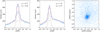 |
Fig. 1. Proper motion distribution of member candidates in the core regions (< 10′ from the centers of h and χ Persei). The proper motion distribution in RA and Dec are shown in the left panel and central panel. Double Gaussian profiles fit the distribution of members (dashed curve) and field stars (dotted curve) separately, while the solid red line shows the combined profiles. Right panel: the red dashed line represents the membership criteria in the proper motion space, which includes the most probable member stars. |
To further purify the member candidates, we used parallax criteria in Fig. 2 to exclude field stars from the 1294 remaining member candidates. In the left panel, the parallax distribution of those stars can be well fitted by a single Gaussian profile, which suggest the contamination by field stars is not significant; we exclude stars with parallax ϖ greater than 2σϖ of the Gaussian distribution. The histogram of relative deviation σϖ/ϖ is shown in the middle panel with the peak located at about 10%. To include the majority of member candidates, we select 15% as the criteria of relative deviation σϖ/ϖ, which makes it contain 68% of remaining member candidates. The σϖ/ϖ versus ϖ diagram of the member candidates is shown in the right panel with blue dots. The parallax criteria is set as a region with σϖ/ϖ less than 15% and ϖ ranging from 0.32 mas to 0.48 mas (red dashed curve). After this parallax selection, the core member candidates retain 768 sources.
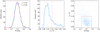 |
Fig. 2. Parallax distribution of core member candidates selected by the proper motion criteria. Left panel: histogram of parallax ϖ that can be fitted by a single Gaussian profile. The distribution of relative deviation of ϖ is shown in the central panel; the red dashed curve represents the acceptable maximum σϖ/ϖ boundary, which includes 68% of the candidates in the histogram. Right panel: the parallax criteria is indicated with the red dashed curve. |
In the G versus GBP − GRP CMD, the limiting boundaries of astrometrically selected possible member candidates were also determined, as shown in Fig. 3. We divide member candidates into several bins along with the G-band magnitude. For each magnitude bin, we use a Gaussian function to fit the stellar color distribution. The range between the lower and upper bounds contains 95% member candidates (2σ clipping in color) and further reduces field stars contamination. To make the boundaries trace the majority of isochrone distribution, we interpolate and smooth the boundaries from 6 mag to 16.5 mag in the G band as is shown in Fig. 3. Finally, in the core regions, 637 core candidates are left after the CMD criteria procedure.
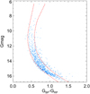 |
Fig. 3. G vs. GBP − GRP CMD for astrometrically selected possible member candidates. The two red dashed lines trace the 95% candidates distribution and are regarded as the CMD criteria to further reducing field stars contamination. |
In summary, any remaining member candidate meets the following criteria: (i) the proper motion must be within a circular region centered on (μα, μδ)=(−0.71, −1.12) mas yr−1 with radius 0.25 mas yr−1 (1σ); (ii) the parallax (ϖ) must be within the region (0.32, 0.48) mas, and its relative deviation of ϖ less than 15%; and (iii) the CMD (GBP − GRP, G mag) must trace the majority of isochrone distribution of core members, as shown in Fig. 3.
3. Results and discussion
After establishing the membership criteria from the core member candidates of h and χ Persei, we performed a member identification process to the initial catalog, which contains more than 9 million sources from Gaia DR2. After applying the selection criteria, 2186 stars are identified as member stars. It is noted that, our purpose in identifying member stars is to explore the extended halo population and substructures of the Double Cluster at large spatial scales. Therefore, it is crucial to have a purer member sample in the trade-off between purity and completeness.
3.1. Spatial distribution
Figure 4 shows the spatial distribution of our member candidates. It is clear that in addition to the central core region of the Double Cluster, a significant number of member stars are spread out over a vast area, extending far beyond the h and χ Persei boundary, as previously suggested by Kharchenko et al. (2013), Dias et al. (2002).
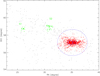 |
Fig. 4. Spatial distribution of member candidates selected using the membership criteria. Based on the classification results from the DBSCAN clustering algorithm, substructure components; halo and core components are indicated as green and red dots, respectively. The solid line represents the core region from Kharchenko et al. (2013). For comparison, the extended halo region in this work is plotted with the dashed curve; 1.5° in radius are centered the Double Cluster centre, which is about 6 − 8 times larger than the core radius of the Double Cluster. |
To further probe the morphology of this extended halo and possible substructures, we adopt the clustering algorithm DBSCAN. This algorithm is widely used to define a set of nearby points in the parameter space as a cluster. The two DBSCAN parameters of define a set of cluster in our work are ϵ = 0.4 and minPts = 14, which represent the radius and minimum number of sources falling into the radius of the hypersphere, respectively (see more detail description in Castro-Ginard et al. 2018, and reference therein).
Figure 4 also shows the DBSCAN classification results. Stars were classified into three groups. The red dots represent the group of cluster members located on the cluster core region and the adjacent halo region. The rest of two cluster groups are considered as cluster substructures and shown as green dots.
3.1.1. Halo population
In much of the literature, the angular size of a star cluster is represented by the core radius, which is easily measured from the marked stellar overdensity features. Kharchenko et al. (2005) suggested a corona radius as the actual radius of a cluster, which is defined as the radius at which the stellar surface density equals the density of surrounding field. In general, the corona radius is about 2.5 times larger than the core radius (Kharchenko et al. 2005).
Based on our member sample selection, the Double Cluster possesses an extended low-density halo, which to our knowledge has never been reported before. Its detection was possible only due to the unique capabilities of Gaia. In Fig. 4, we plot the angular radius of the core region (r1, from the catalog of Kharchenko et al. 2013) as the blue circle. For contrast, we also plot a dashed blue circle that is 1.5° in radius around the cluster common center. It is clear that our results show a more extended region for both h and χ Persei that is about six to eight times larger than their core radius. However, because of the incompleteness of the member sample, the halo radius of the Double Cluster is still regarded as a lower limit of the actual radius, even though the halo radius extends greatly beyond what was previously expected.
3.1.2. Substructures
The most surprising discovery are the long-stretching filamentary substructures of the Double Cluster, which are shown in Fig. 4 (denoted as S1 and S2). Although substructures have been observed in massive star-forming regions (Lada & Lada 2003), the scale size and extended length of cluster samples are much smaller than those of the Double Cluster, even for the linear chains of clusters classified in Kuhn et al. (2014), whose scale length ranges from 10 pc to 30 pc. For the substructures S1 and S2 (see Fig. 4), the angular radius between the common centre of the Double Cluster and the centre of substructures are 5.1°, and 2.9°, corresponding to projected distances extending to 208 pc and 118 pc, respectively (with an adopted cluster distance of 2344 pc; Currie et al. 2010).
Kinematic information can provide hints about the origin of the substructures. The relative tangential velocity between the substructures and cores of the Double Cluster are about 2 km s−1 (see below). This means even for the nearest substructure S2, it would take about 60 Myr to form this structure, if we assume that stars in S2 originate from the Double Cluster. This formation time greatly exceeds the Double Cluster age of 14 Myr (Currie et al. 2010). Therefore, these substructures are more likely to be primordial structures that have formed together with the Double Cluster core, instead of a tidally disrupted stream from the cluster center.
3.2. Properties of double cluster components
In Fig. 5 we plot the total proper motion (top panel) and parallax (bottom panel) distribution of each component to study the physical properties of three major Double Cluster components that are labeled by the DBSCAN; these include the cluster cores, halo population, and substructures. Different colors represent different components: h Persei in red, χ Persei in green, halo population in yellow, S1 in blue, and S2 in violet. The Gaussian function is used to fit the histogram of each component. Fitting results of proper motion and parallax distribution are shown in Table 1. The similar proper motion distribution and dispersion suggest the coeval feature of Double Cluster components. We note that the parallax fitting results show that the line of sight distance between core components and substructures are about 291 pc and 125 pc for S1 and S2, respectively; these are comparable with the projected distances (see Sect. 3.1.2).
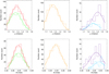 |
Fig. 5. Proper motion and parallax distribution of each component identified by the DBSCAN. Colored lines indicate Double Cluster components, including h Persei (red), χ Persei (green), the halo population (yellow), S1 (blue), and S2 (violet). A Gaussian function is also applied to fit the histogram of each component. The fitted results are shown in Table 1. |
Gaussian fit results of parameters distribution.
Furthermore, it is important to constrain the age of stars belonging to different components. Figure 6 shows the isochrone fitting result for three major components; the same color indicators are used as in Fig. 5. Referring to the literature estimation of age of the Double Cluster (Currie et al. 2010), we adopt the 14 Myr isochrone (log[t/yr] = 7.14) with solar abundance from Padova stellar evolution models to perform the visual fit.
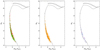 |
Fig. 6. Dereddened MG vs. (GBP − GRP)0 CMD for three major components labeled by the DBSCAN. Colors are the same as in Fig. 5. The Padova isochrone of 14 Myr is overlaid on the CMDs of three major components. |
To transform the observational magnitude (G) and colors (GBP − GRP) of each star to the absolute magnitude MG and intrinsic colors (GBP − GRP)0, the distance modulus and reddening need to be determined. For each component, the Gaia DR2 provides reliable parallax measurements. The parallax of stars are used to derive their individual distance modulus. The only free parameter to adjust the isochrone fitting is the reddening E(B − V). The extinction AG and reddening E(BP − RP) are calculated as AG = RG × E(B − V) and E(BP − RP)=(RBP − RRP) × E(B − V), where RG = 2.740, RBP = 3.374 and RRP = 2.035, respectively (Casagrande & VandenBerg 2018). In our work, the best-fitting isochrone is derived from the average E(B − V) = 0.65 for three major components, which is slightly higher than the results of Currie et al. (2010); Slesnick et al. (2002). However, considering the dispersion of reddening for different spectral type, our results are still within a reasonable range.
3.3. Internal kinematic distribution
Most of the stars in our member sample have a brightness in the range of G = 13 − 17 mag, and none of the members has radial velocity measurement in Gaia DR2. In this work, we therefore only use proper motion parameters to perform the kinematic analysis.
In our sample of Double Cluster members, the measurement uncertainty of proper motion is small and has mean uncertainties 0.08 ± 0.03 mas yr−1 in pmRA and 0.09 ± 0.03 mas yr−1 in pmDE. Assuming all member stars have nearly the same distance, i.e., d ≈ 2.3 kpc (Currie et al. 2010), the tangential velocities of our sample stars range from −10.7 km s−1 to −5.2 km s−1 in RA and −15.2 km s−1 to −9.8 km s−1 in Dec, and the mean values are −7.7 ± 1.2 km s−1 in RA and −12.2 ± 1.2 km s−1 in Dec, respectively.
To study the stellar relative motions in the tangential direction, especially for the internal motions within the core, halo, and substructure populations, we assume the bulk motions of core members as the zero point and estimate the average tangential velocity of core members first. In our sample, stars within radius of 0.24° to the h Persei center and radius of 0.175° to the χ Persei center (Kharchenko et al. 2013) are defined as core members. The average tangential velocity of core members is −7.5 ± 1.1 km s−1 in RA and −12.3 ± 1.1 km s−1 in Dec, nearly equal to the mean tangential velocity of all members. We then subtract the average tangential velocity from the all member stars. The residual velocity values can be considered as internal motions in the core region.
To distinguish the relative tangential velocity of different populations, we study the relative motions of member stars. For simplicity, we categorize cluster members into four quadrant samples, according to their proper motion directions. We plot a map with the projected coordinate system to show the spatial distribution of member stars using different colors, which represent their relative velocity directions belonging to different quadrants. To make the populations more distinguishable, the most crowded core regions were excluded in Fig. 7.
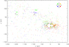 |
Fig. 7. Locations of member stars with different internal motion directions on the projected coordinate system, whose origin is located at the common center of the Double Cluster core. With the mean tangential velocity of core members as its zero point, stars are categorized into four samples according to their residual tangential velocity direction, as plotted with different colors. Arrows close to the label of S1 and S2 point out the average internal motion direction of substructure members. The almost orthogonal motion direction suggests the possibility of different dynamical formation histories of these two substructures. |
In Fig. 7, for stars in S1 and S2 substructure areas, we select stars within the same quadrant sample to calculate the average tangential velocities as 2.2 ± 0.6 km s−1 and 1.9 ± 0.7 km s−1 for S1 and S2, respectively. The arrows indicate the average velocity directions. Similarly, the averaged velocity direction (angles in degrees, measured counterclockwise from the positive X coordinate) of the S1 and S2 subsamples are 148 ° ±25° and 227 ° ±25°, respectively.
In contrast to the bulk movements of the substructures, the tangential velocity distribution of the halo members and core members is more complex. For different velocity samples, we calculate their mean spatial position and dispersion. Figure 8 shows the projection map of core and halo members. The colors represent different velocity samples as shown in Fig. 7, and the solid circles and error bars represent the mean position and position dispersion of stars in each sample. The spatial distribution of halo stars in the various samples is shown in the left panel of Fig. 8. The offset of the mean positions for each sample shows that stars with velocity in the first and fourth quadrants tend to be located in the positive region. In contrast, stars with velocities in the second and third quadrants are located in a relatively negative region. It seems that exhibiting a bulk motion away from the cluster cores, the structure of the halo star population is experiencing certain dynamic stretching effect in the X (RA) direction.
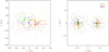 |
Fig. 8. Locations of halo (left panel) and core (right panel) components with different internal motion directions on the projected coordinate system, whose origin is located at the common center of the Double Cluster core. Colors are identical to those in Fig. 7. The solid circles and their corresponding error bars represent the mean position and spatial dispersion of each sample, respectively. For halo and core components, the different position distribution of the four motion direction samples suggests that the tidal stripping event occurs on the outskirts of the Double Cluster, while the influence on core components is relatively small. |
On the other hand, in the core region the spatial distributions of the four velocity samples are similar and have no inclined direction, as shown in the bottom panel of Fig. 8. For member stars in the core region, the tangential velocity dispersion is 0.6 km s−1 for both h and χ Persei. Such a small intrinsic velocity dispersion suggests the existence of dynamically compact cores in the Double Cluster.
The clusters h and χ Persei have masses of roughly 5500 M⊙ and 4300 M⊙, respectively (Bragg & Kenyon 2005), and the corresponding tidal radii are (depending on the exact masses) roughly 23 pc. The half-mass relaxation time of both clusters is of order 100 Myr (Bragg & Kenyon 2005), which is substantially longer than the age of either of the star clusters. Consequently, the effects of two-body relaxation and subsequent stellar ejections from the cluster cores are limited. We carry out N-body simulations using NBODY6++GPU (Wang et al. 2015, 2016) and find that only a handful of stars (primarily neutron stars that experienced a velocity kick) are ejected beyond the tidal radius within the age of the star clusters, while the effect of the Galactic external tidal field does not result in escape through evaporation on this timescale. Conversely, a much larger number of stars are found in the Double Star cluster halo. The different dynamical properties of core and halo population imply that only the tidal stripping event had a significant influence on the outskirts of the Double Cluster, while the impact on the core components is relatively small.
To further clarify the intrinsic velocity offset in the X coordinate, we classify halo and core members into two velocity groups: a red group with positive RA proper motions and a green group with negative RA proper motions. The projected spatial distribution of the two velocity groups are shown in Fig. 9. The distribution pattern in Fig. 9 also demonstrates that stars with positive RA proper motions tend to be located in the positive region in X coordinate, while stars with negative RA proper motions tend to be located in the negative region in X coordinate.
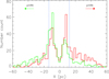 |
Fig. 9. Histograms of the different velocity groups in X coordinates. The red histograms represent stars with RA proper motion along the X direction and the green histograms represent stars with RA proper motion opposite from the X coordinates. The region between two blue dash lines indicates the Double Cluster core region (Kharchenko et al. 2013). To show the histogram of stars belonging to cluster cores, halo stars were excluded whose position happens to be the locus of the core region in X coordinates (the region enclosed by the blue vertical lines). |
4. Summary
We have studied the extended spatial morphology and kinematic properties of the Double Cluster h and χ Persei, using unprecedented high-precision data from the Gaia DR2. As suggested by Currie et al. (2010), an extended halo structure has been found at an angular distance beyond one degree from the Double Cluster core. Furthermore, a long-stretching filamentary substructure is discovered for the first time, which extends to a projected distance of more than 200 pc away from the Double Cluster centre. These extended structures suggest that cluster formation mode and its history may be more complex than previously expected.
Based on our internal kinematic analysis, the small tangential velocity between substructure and cluster core implies that filamentary substructures are more likely to be primordial structures, reminiscent from the star formation event that formed the Double Cluster. In addition, for members in the halo region, the tangential velocity distribution suggests that a tidal stripping event is occurring in the outskirts of the Double Cluster. By contrast, core components of the Double Cluster still maintain the dynamical compact properties.
Although the Gaia spectroscopic data is absent in our kinematic analysis, the ongoing LAMOST-MRS survey (LAMOST Collaboration et al. in prep.) is arranged to observe a large number of member sources in the Double Cluster field within a 5° diameter. More than 20 000 medium-resolution stellar spectra (R ∼ 7500, σRV ∼ 1 − 2 km s−1) are expected to be provided by the LAMOST-MRS survey, while the completeness of cluster member stars (bpmag ≤ 15 mag) can reach to about 80%. After combining the LAMOST data and Gaia data, the three-dimensional internal kinematic properties of cluster components as well as the metallicity distribution can be studied in further detail.
Acknowledgments
The authors acknowledge the National Natural Science Foundation of China (NSFC) under grants U1731129 and 11503066 (PI: Zhong), 11373054 and 11661161016 (PI: Chen), 11390373 (PI: Shao). M.B.N.K. acknowledges support from the National Natural Science Foundation of China (grant 11573004) and the Research Development Fund (grant RDF-16-01-16) of Xi’an Jiaotong-Liverpool University (XJTLU). This project was developed in part at the 2018 Gaia-LAMOST Sprint workshop, supported by the National Natural Science Foundation of China (NSFC) under grants 11333003. This work has made use of data from the European Space Agency (ESA) mission Gaia (https://www.cosmos.esa.int/gaia), processed by the Gaia Data Processing and Analysis Consortium (DPAC, https://www.cosmos.esa.int/web/gaia/dpac/consortium). Funding for the DPAC has been provided by national institutions, in particular the institutions participating in the Gaia Multilateral Agreement.
References
- Bailer-Jones, C. A. L., Rybizki, J., Fouesneau, M., Mantelet, G., & Andrae, R. 2018, AJ, 156, 58 [NASA ADS] [CrossRef] [Google Scholar]
- Bragg, A. E., & Kenyon, S. J. 2002, AJ, 124, 3289 [NASA ADS] [CrossRef] [Google Scholar]
- Bragg, A. E., & Kenyon, S. J. 2005, AJ, 130, 134 [NASA ADS] [CrossRef] [Google Scholar]
- Cantat-Gaudin, T., Jordi, C., Vallenari, A., et al. 2018, A&A, 618, A93 [NASA ADS] [CrossRef] [EDP Sciences] [Google Scholar]
- Casagrande, L., & VandenBerg, D. A. 2018, MNRAS, 479, L102 [NASA ADS] [CrossRef] [Google Scholar]
- Castro-Ginard, A., Jordi, C., Luri, X., et al. 2018, A&A, 618, A59 [NASA ADS] [CrossRef] [EDP Sciences] [Google Scholar]
- Currie, T., Balog, Z., Kenyon, S. J., et al. 2007, ApJ, 659, 599 [NASA ADS] [CrossRef] [Google Scholar]
- Currie, T., Hernandez, J., Irwin, J., et al. 2010, ApJS, 186, 191 [NASA ADS] [CrossRef] [MathSciNet] [Google Scholar]
- Dias, W. S., Alessi, B. S., Moitinho, A., & Lépine, J. R. D. 2002, A&A, 389, 871 [NASA ADS] [CrossRef] [EDP Sciences] [Google Scholar]
- Evans, II., N. J., Dunham, M. M., Jørgensen, J. K., et al. 2009, ApJS, 181, 321 [NASA ADS] [CrossRef] [Google Scholar]
- Faesi, C. M., Lada, C. J., & Forbrich, J. 2016, ApJ, 821, 125 [NASA ADS] [CrossRef] [Google Scholar]
- Gaia Collaboration (Prusti, T., et al.) 2016, A&A, 595, A1 [NASA ADS] [CrossRef] [EDP Sciences] [Google Scholar]
- Gaia Collaboration (Brown, A. G. A., et al.) 2018, A&A, 616, A1 [NASA ADS] [CrossRef] [EDP Sciences] [Google Scholar]
- Garmany, C. D., & Stencel, R. E. 1992, A&AS, 94, 211 [NASA ADS] [Google Scholar]
- Heyer, M., & Dame, T. M. 2015, ARA&A, 53, 583 [NASA ADS] [CrossRef] [Google Scholar]
- Kharchenko, N. V., Piskunov, A. E., Röser, S., Schilbach, E., & Scholz, R.-D. 2005, A&A, 438, 1163 [NASA ADS] [CrossRef] [EDP Sciences] [MathSciNet] [Google Scholar]
- Kharchenko, N. V., Piskunov, A. E., Schilbach, E., Röser, S., & Scholz, R.-D. 2013, A&A, 558, A53 [NASA ADS] [CrossRef] [EDP Sciences] [Google Scholar]
- Kuhn, M. A., Feigelson, E. D., Getman, K. V., et al. 2014, ApJ, 787, 107 [Google Scholar]
- Lada, C. J., & Lada, E. A. 2003, ARA&A, 41, 57 [NASA ADS] [CrossRef] [Google Scholar]
- Lada, E. A., Strom, K. M., & Myers, P. C. 1993, Protostars and Planets, III [Google Scholar]
- Luo, A.-L., Zhao, Y.-H., Zhao, G., et al. 2015, Res. Astron. Astrophys., 15, 1095 [NASA ADS] [CrossRef] [Google Scholar]
- Marsh Boyer, A. N., McSwain, M. V., Aragona, C., & Ou-Yang, B. 2012, AJ, 144, 158 [NASA ADS] [CrossRef] [Google Scholar]
- Oosterhoff, P. T. 1937, Ann. van de Sterrewacht te Leiden, 17, A1 [NASA ADS] [Google Scholar]
- Portegies Zwart, S. F., McMillan, S. L. W., & Gieles, M. 2010, ARA&A, 48, 431 [NASA ADS] [CrossRef] [Google Scholar]
- Priyatikanto, R., Kouwenhoven, M. B. N., Arifyanto, M. I., Wulandari, H. R. T., & Siregar, S. 2016, MNRAS, 457, 1339 [Google Scholar]
- Rastorguev, A. S., Glushkova, E. V., Dambis, A. K., & Zabolotskikh, M. V. 1999, Astron. Lett., 25, 595 [NASA ADS] [Google Scholar]
- Slesnick, C. L., Hillenbrand, L. A., & Massey, P. 2002, ApJ, 576, 880 [NASA ADS] [CrossRef] [Google Scholar]
- Uribe, A., García-Varela, J. A., Sabogal-Martínez, B. E., Higuera, G. M. A., & Brieva, E. 2002, PASP, 114, 233 [NASA ADS] [CrossRef] [Google Scholar]
- Xiang, M. S., Liu, X. W., Yuan, H. B., et al. 2015, MNRAS, 448, 822 [NASA ADS] [CrossRef] [Google Scholar]
- Wang, L., Spurzem, R., Aarseth, S., et al. 2015, MNRAS, 450, 4070 [NASA ADS] [CrossRef] [Google Scholar]
- Wang, L., Spurzem, R., Aarseth, S., et al. 2016, MNRAS, 458, 1450 [NASA ADS] [CrossRef] [Google Scholar]
- Zhao, G., Zhao, Y.-H., Chu, Y.-Q., Jing, Y.-P., & Deng, L.-C. 2012, Res. Astron. Astrophys., 12, 723 [NASA ADS] [CrossRef] [Google Scholar]
All Tables
All Figures
|
Fig. 1. Proper motion distribution of member candidates in the core regions (< 10′ from the centers of h and χ Persei). The proper motion distribution in RA and Dec are shown in the left panel and central panel. Double Gaussian profiles fit the distribution of members (dashed curve) and field stars (dotted curve) separately, while the solid red line shows the combined profiles. Right panel: the red dashed line represents the membership criteria in the proper motion space, which includes the most probable member stars. |
| In the text | |
|
Fig. 2. Parallax distribution of core member candidates selected by the proper motion criteria. Left panel: histogram of parallax ϖ that can be fitted by a single Gaussian profile. The distribution of relative deviation of ϖ is shown in the central panel; the red dashed curve represents the acceptable maximum σϖ/ϖ boundary, which includes 68% of the candidates in the histogram. Right panel: the parallax criteria is indicated with the red dashed curve. |
| In the text | |
|
Fig. 3. G vs. GBP − GRP CMD for astrometrically selected possible member candidates. The two red dashed lines trace the 95% candidates distribution and are regarded as the CMD criteria to further reducing field stars contamination. |
| In the text | |
|
Fig. 4. Spatial distribution of member candidates selected using the membership criteria. Based on the classification results from the DBSCAN clustering algorithm, substructure components; halo and core components are indicated as green and red dots, respectively. The solid line represents the core region from Kharchenko et al. (2013). For comparison, the extended halo region in this work is plotted with the dashed curve; 1.5° in radius are centered the Double Cluster centre, which is about 6 − 8 times larger than the core radius of the Double Cluster. |
| In the text | |
|
Fig. 5. Proper motion and parallax distribution of each component identified by the DBSCAN. Colored lines indicate Double Cluster components, including h Persei (red), χ Persei (green), the halo population (yellow), S1 (blue), and S2 (violet). A Gaussian function is also applied to fit the histogram of each component. The fitted results are shown in Table 1. |
| In the text | |
|
Fig. 6. Dereddened MG vs. (GBP − GRP)0 CMD for three major components labeled by the DBSCAN. Colors are the same as in Fig. 5. The Padova isochrone of 14 Myr is overlaid on the CMDs of three major components. |
| In the text | |
|
Fig. 7. Locations of member stars with different internal motion directions on the projected coordinate system, whose origin is located at the common center of the Double Cluster core. With the mean tangential velocity of core members as its zero point, stars are categorized into four samples according to their residual tangential velocity direction, as plotted with different colors. Arrows close to the label of S1 and S2 point out the average internal motion direction of substructure members. The almost orthogonal motion direction suggests the possibility of different dynamical formation histories of these two substructures. |
| In the text | |
|
Fig. 8. Locations of halo (left panel) and core (right panel) components with different internal motion directions on the projected coordinate system, whose origin is located at the common center of the Double Cluster core. Colors are identical to those in Fig. 7. The solid circles and their corresponding error bars represent the mean position and spatial dispersion of each sample, respectively. For halo and core components, the different position distribution of the four motion direction samples suggests that the tidal stripping event occurs on the outskirts of the Double Cluster, while the influence on core components is relatively small. |
| In the text | |
|
Fig. 9. Histograms of the different velocity groups in X coordinates. The red histograms represent stars with RA proper motion along the X direction and the green histograms represent stars with RA proper motion opposite from the X coordinates. The region between two blue dash lines indicates the Double Cluster core region (Kharchenko et al. 2013). To show the histogram of stars belonging to cluster cores, halo stars were excluded whose position happens to be the locus of the core region in X coordinates (the region enclosed by the blue vertical lines). |
| In the text | |
Current usage metrics show cumulative count of Article Views (full-text article views including HTML views, PDF and ePub downloads, according to the available data) and Abstracts Views on Vision4Press platform.
Data correspond to usage on the plateform after 2015. The current usage metrics is available 48-96 hours after online publication and is updated daily on week days.
Initial download of the metrics may take a while.