Growth after the streaming instability

Beibei Liu; Chris W. Ormel; Anders Johansen

doi:10.1051/0004-6361/201834174

Home

All issues

Volume 624 (April 2019)

A&A, 624 (2019) A114

Full HTML

Free Access

Issue		A&A Volume 624, April 2019


Article Number		A114
Number of page(s)		14
Section		Planets and planetary systems
DOI		https://doi.org/10.1051/0004-6361/201834174
Published online		22 April 2019

A&A 624, A114 (2019)

From planetesimal accretion to pebble accretion

Beibei Liu (刘倍贝)¹^,2, Chris W. Ormel² and Anders Johansen¹

¹ Lund Observatory, Department of Astronomy and Theoretical Physics, Lund University, Box 43, 22100 Lund, Sweden
e-mail: bbliu@astro.lu.se; anders@astro.lu.se
² Anton Pannekoek Institute (API), University of Amsterdam, Science Park 904, 1090GE Amsterdam, The Netherlands
e-mail: c.w.ormel@uva.nl

Received: 2 September 2018
Accepted: 26 February 2019

Abstract

Context. Streaming instability is a key mechanism in planet formation, clustering pebbles into planetesimals with the help of self-gravity. It is triggered at a particular disk location where the local volume density of solids exceeds that of the gas. After their formation, planetesimals can grow into protoplanets by feeding from other planetesimals in the birth ring as well as by accreting inwardly drifting pebbles from the outer disk.

Aims. We aim to investigate the growth of planetesimals into protoplanets at a single location through streaming instability. For a solar-mass star, we test the conditions under which super-Earths are able to form within the lifetime of the gaseous disk.

Methods. We modified the Mercury N-body code to trace the growth and dynamical evolution of a swarm of planetesimals at a distance of 2.7 AU from the star. The code simulates gravitational interactions and collisions among planetesimals, gas drag, type I torque, and pebble accretion. Three distributions of planetesimal sizes were investigated: (i) a mono-dispersed population of 400 km radius planetesimals, (ii) a poly-dispersed population of planetesimals from 200 km up to 1000 km, (iii) a bimodal distribution with a single runaway body and a swarm of smaller, 100 km size planetesimals.

Results. The mono-dispersed population of 400 km size planetesimals cannot form protoplanets of a mass greater than that of the Earth. Their eccentricities and inclinations are quickly excited, which suppresses both planetesimal accretion and pebble accretion. Planets can form from the poly-dispersed and bimodal distributions. In these circumstances, it is the two-component nature that damps the random velocity of the large embryo through the dynamical friction of small planetesimals, allowing the embryo to accrete pebbles efficiently when it approaches 10⁻² M_⊕. Accounting for migration, close-in super-Earth planets form. Super-Earth planets are likely to form when the pebble mass flux is higher, the disk turbulence is lower, or the Stokes number of the pebbles is higher.

Conclusions. For the single site planetesimal formation scenario, a two-component mass distribution with a large embryo and small planetesimals promotes planet growth, first by planetesimal accretion and then by pebble accretion of the most massive protoplanet. Planetesimal formation at single locations such as ice lines naturally leads to super-Earth planets by the combined mechanisms of planetesimal accretion and pebble accretion.

Key words: methods: numerical / planets and satellites: formation

© ESO 2019

1 Introduction

In protoplanetary disks, micrometer-sized dust grains coagulate into pebbles of millimeter to centimeter sizes (Dominik & Tielens 1997; Birnstiel et al. 2012; Krijt et al. 2016; Pérez et al. 2015; Tazzari et al. 2016). However, further growth is suppressed by bouncing or fragmentation due to the increasing compactification in collisions (Güttler et al. 2010; Zsom et al. 2010). In addition, these pebbles also drift too fast compared to their growth (Weidenschilling 1977) so that the particles cannot cross the meter size barrier even if they would stick perfectly (Birnstiel et al. 2012; Lambrechts & Johansen 2014), unless the pebbles can remain fluffy during the growth (Okuzumi et al. 2012; Kataoka et al. 2013). The subsequent growth of these pebbles into planetesimals is still not well understood in planet formation theory (see Johansen et al. 2014 for a review).

The streaming instability mechanism provides a promising solution by concentrating drifting pebbles due to a locally enhanced solid-to-gas ratio. Once the threshold of solid-to-gas ratio is satisfied, the pebble clumps can directly collapse into planetesimals (Youdin & Goodman 2005; Johansen et al. 2007, 2009; Bai & Stone 2010). The characteristic size of these planetesimals is approximately a few hundred kilometres (Johansen et al. 2012, 2015; Simon et al. 2016, 2017; Schäfer et al. 2017; Abod et al. 2018).

The subsequent growth after planetesimal formation by streaming instability has not been well studied. These newly born planetesimals could interact with each other. In the classical planetesimal accretion scenario (see Raymond et al. 2014; Izidoro & Raymond 2018 for reviews), the gravitational interactions among these planetesimals lead to orbital crossings, scatterings, and collisions. Initially, the velocity dispersions of planetesimals are not strongly excited and remain modest. At this stage the accretion is super linear ( $d m_{p} / d t \propto m_{p}^{γ}$ $\textrm{d}m_{\textrm{p}}/\textrm{d}t \propto m_{\textrm{p}}^{\gamma}$ with γ > 1), which is termed “runaway growth” (Greenberg et al. 1978; Wetherill & Stewart 1989; Ida & Makino 1993; Kokubo & Ida 1996; Rafikov 2004; Ida & Lin 2004). It means that the massive body has a faster accretion rate and therefore will quickly become more massive. However, this stage cannot last forever. Since the growing massive bodies would stir the random velocities of neighboring small planetesimals, the accretion rates of the massive bodies slow down and turn into a self-limiting mode. This phase is called “oligarchic growth” where $d m_{p} / d t \propto m_{p}^{γ}$ $\textrm{d}m_{\textrm{p}}/\textrm{d}t \propto m_{\textrm{p}}^{\gamma}$ with γ < 1 (Kokubo & Ida 1998). This phase is characterized by a decreasing mass ratio of two adjacent massive runaway bodies (Lissauer 1987; Kokubo & Ida 2000; Thommes et al. 2003; Ormel et al. 2010).

In addition to planetesimal accretion, planetesimals formed by streaming instability can accrete inward drifting pebbles. A planetesimal may capture a fraction of the pebbles that cross its orbit (Ormel & Klahr 2010; Lambrechts & Johansen 2012). This is known as pebble accretion (see recent reviews by Johansen & Lambrechts 2017; Ormel 2017). Even if only a fraction of pebbles are able to be accreted by planets, the pebble accretion rate can still be high for two reasons. First, the accretion cross section is significantly enhanced by gas drag (Ormel & Klahr 2010); and second, a large flux of pebbles grow and drift inward from the outer regions of disks (Birnstiel et al. 2012; Lambrechts & Johansen 2014). Pebble accretion can be classified into 2D/3D regimes (Ormel & Klahr 2010; Morbidelli et al. 2015). When the pebble accretion radius is larger than the pebble scale height, the accretion is in the 2D regime, where $d m_{p} / d t \propto m_{p}^{2 / 3}$ $\textrm{d}m_{\textrm{p}}/\textrm{d}t \propto m_{\textrm{p}}^{2/3}$ (Lambrechts & Johansen 2014, Hill regime). On the other hand, when the pebble scale height exceeds the pebble accretion radius, only pebbles with heights smaller than the accretion radius can be accreted. Therefore, the accretion rate in this 3D regime is reduced compared to2D, and d m_p∕dt ∝ m_p (Ida et al. 2016).

In general, the efficacy of the pebble accretion mechanism to grow planet(esimals) depends on many variables related to the properties of the disk, pebble, and planet (the eccentricity, the inclination, and the mass of the planet, the pebble size, the disk turbulence, etc.) A key quantity is the pebble accretion efficiency ε_PA (Guillot et al. 2014; Lambrechts & Johansen 2014), defined as the number of pebbles that are accreted divided by the total number of pebbles that the disk supplies. Recently we have computed ε_PA under general circumstances (Liu & Ormel 2018; Ormel & Liu 2018). For instance, when the eccentricity and inclination of the planet become high, ε_PA drops significantly compared to planets on coplanar and circular orbits, because pebbles are approaching the planet at a too high velocity.

Progress in planet formation requires an improved understanding of under which conditions the mass growth is dominated by accreting pebbles or planetesimals. In this work, our goal is to investigate the growth of planetesimals after their formation by streaming instability at a single disk location (e.g., the H₂ O ice line). Hansen (2009) already proposed that the architecture of the solar system’s terrestrial planets can be explained when planetesimals grow in a narrow annulus. In his model the width of the annulus is 0.3 AU, much wider than our planetesimal forming zone (see Sect. 2). Furthermore, Hansen (2009) focused on the planetesimal accretion in a gas-free environment. Our work instead considers the growth just after the streaming instability in the gas-rich disk phase.

Constrained by the size distribution of planetesimals in the asteroid belt, Morbidelli et al. (2009) concluded that their born size should be large (≳100 km), while Weidenschilling (2011) argued that planetesimals starting from sub-kilometer-sized still cannot be ruled out. Kenyon & Bromley (2010) studied the formation of ice planets beyond 30 AU and found that protoplanets grow more efficiently with smaller planetesimal sizes. Motivated by streaming instability simulations, our adopted initial sizes are typically ≳100 km. In the context of combined planetesimal and pebble accretion, Johansen et al. (2015) studied the growth of asteroids using a statistical approach, and concluded that massive protoplanets or even super-Earths can form by a combination of pebble accretion, planetesimal accretion, and giant impacts.

In order to study planet formation from a narrow ring of planetesimals, we employ direct N-body techniques. Growth can be classified into two phases: (A) the planetesimal accretion dominated phase and (B) the pebble accretion dominated phase. The N-body approach is necessary to treat phase A and the transition from phase A to phase B. The Mercury N-body code has been modified to include gas drag, type I torque, and pebble accretion. Three different types of initial planetesimal size distributions were investigated. We find that a two-component mass distribution (large embryo + small planetesimals) is needed to grow a massive planet. This condition could arise either from the high mass tail distribution of planetesimals formed by streaming instability or be the result of runaway growth of a population of small planetesimals.

The paper is structured as follows. In Sect. 2, we outline our model and the implementation of the N-body code. In Sect. 3 three initial size distributions of planetesimals are investigated, including a mono-dispersed population in Sect. 3.1, a poly-dispersed population in Sect. 3.2, and a single runaway body plus a swarm of small planetesimals in Sect. 3.3. In Sect. 4 we investigate the influence of different parameters in the pebble accretion dominated growth phase (phase B). The key results are summarized in Sect. 5.

2 Method

The hypothesis of this paper is that planetesimals only form at a specific location by streaming instability, which requires a locally enhanced pebble density (Carrera et al. 2015; Yang & Johansen 2014; Yang et al. 2017, 2018). For instance, Ros & Johansen (2013), Schoonenberg & Ormel (2017) and Dra̧żkowska & Alibert (2017) have proposed that the ice line could be such a place since the water vapor inside the ice line will diffuse back and re-condense onto ice pebbles, enriching the solid-to-gas density ratio. We focus on planetesimals that form at the ice line (r_ice = 2.7 AU based on the disk model in Sect. 2.1) in this paper. However, the following results and applications can be scaled to other locations where the streaming instability condition is realized, for example, the inner edge of the zone (Chatterjee & Tan 2014; Hu et al. 2018) or a distant location due to photoevaporation (Carrera et al. 2017). In order to generalize our results, we did not include the specific ice line effects such as a reduced pebble size and pebble flux inside of the ice line due to sublimation.

This scenario is illustrated in Fig. 1. We consider the situation where streaming instability operates to quickly spawn planetesimals at the initial time of our simulations. A population of planetesimals has formed in a narrow annulus of relative width equal to the normalized pressure gradient (Δr = ηr, see Fig. 1 and further discussion in Sect. 2.3). These planetesimals can grow further in two ways: by coagulation among themselves (planetesimal accretion) or by sweeping up pebbles that drift in from the outer disk (pebble accretion).

2.1 Disk model

The surface density and the aspect ratio of the gas disk are assumed to be $Σ_{gas} = Σ_{gas0} {(\frac{r}{1 AU})}^{- 1},$ $\begin{equation*} \Sigma_{\textrm{gas}} \,{=}\, \Sigma_{\textrm{gas0}} \left( \frac{r}{1 \ \textrm{AU}} \right)^{-1},\end{equation*}$ (1) $h_{gas} = h_{gas0} {(\frac{r}{1 AU})}^{1 / 4},$ $\begin{equation*} h_{\textrm{gas}} = h_{\textrm{gas0}} \left( \frac{r}{1 \ \textrm{AU}} \right)^{1/4},\vspace*{-2pt}\end{equation*}$ (2)

where Σ_gas0 and h_gas0 are the gas surface density and the aspect ratio at 1 AU, and r is the distance to the central star. The aspect ratio index of 1/4 assumes an optically thin stellar irradiated disk. For simplicity, we neglect the fact that in the early stages disks might be hotter due to viscous accretion (Garaud & Lin 2007; Kretke & Lin 2012; Bitsch et al. 2015). Here Σ_gas0 = 500 g cm⁻² and h_gas0 = 0.033 (Hayashi 1981) are adopted as the default values in this paper. Therefore, the disk temperature T and η are $T = \frac{μ h_{gas}^{2} G M_{⋆}}{r R_{g}} = T_{0} {(\frac{r}{1 AU})}^{- 1 / 2},$ $\begin{equation*} T = \frac{ \mu h_{\textrm{gas}}^2 G M_{\star}}{r R_{\textrm{g}}} = T_0 \left( \frac{r}{1 \ \textrm{AU}} \right)^{-1/2},\end{equation*}$ (3)

and $η = - \frac{h_{gas}^{2}}{2} \frac{\partial log P_{gas}}{\partial log r} = η_{0} {(\frac{r}{1 AU})}^{1 / 2},$ $\begin{equation*} \eta = -\frac{h_{\textrm{gas}}^2}{2} \frac{\partial {\textrm{log}} P_{\textrm{gas}} }{ \partial {\textrm{log}} r} = \eta_0 \left( \frac{r}{1 \ \textrm{AU}} \right)^{1/2},\end{equation*}$ (4)

where G is the gravitational constant, R_g = 8.31 × 10⁷ erg mol⁻¹ K⁻¹ is the gas constant, M_⋆ is the stellar mass, μ = 2.34 is the mean molecular weight, and P_gas is the gas pressure in the disk. In the above equations, T₀ = 280 K and η₀ = 1.5 × 10⁻³ are the values at 1 AU.

Although the adopted surface density power-law index is shallower than the minimum mass solar nebula model, this profile (Σ_g ∝ r⁻¹) is more consistent with disk observations (Andrews et al. 2009). The fiducial value of Σ_gas0 is chosen to be the same as Lambrechts & Johansen (2014), and the pebble flux is calibrated accordingly in Sect. 2.2.2. Based on the above disk model, the ice line (T ~ 170 K) is located at r_ice = 2.7 AU.

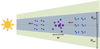Fig. 1

Sketch illustrating the initial setup. Planetesimals (purple circles) have formed at a single location by streaming instability. They accrete both among themselves as well as from the inward drifting pebbles (blue). The pebble disk and gas disk are marked in light blue and light green, where the gas and pebble scale heights are H_gas and H_peb, respectively. The horizontal black arrow represents the radial width (ηr) of the forming planetesimal ring. Due to dynamical friction, large planetesimals have low eccentricities and inclinations whereas small planetesimals have high velocity dispersions.

2.2 Simulation setup

We used numerical N-body simulations to study the planetesimal growth after the streaming instability during the gas-rich disk phase. We have adopted the Mercury code (Chambers 1999) and used the Bulirsch-Stoer integrator. An initial timestep of three days and the integration accuracy parameter of 10⁻¹² were chosen.

For the N-body part, collisions between bodies are treated as inelastic mergers that conserve the linear momentum. Fragmentation and restitution (Leinhardt & Stewart 2012; Mustill et al. 2018) are not taken into account in this work. Since eccentricities are initially low, the perfect merger assumption is appropriate. For instance, the impact velocity of 400-km-sized planetesimals is lower than the escape velocity when their eccentricities are lower than a few times 10⁻². Fragmentation among planetesimals will become important after embryos form and stir the planetesimals more vigorously. However, by then pebble accretion is already expected to commence, rendering planetesimal fragmentation irrelevant.

The effects of the disk gas on the planetesimals and planets, such as gas drag, type I torque, eccentricity, and inclination damping are taken into account by applying effective forces in Sect. 2.2.1. In Sect. 2.2.2, we implement the pebble accretion prescriptions by Liu & Ormel (2018) and Ormel & Liu (2018), which account for the effects of the planet’s eccentricity, inclination, and the disk turbulence. The modified code uniquely simulates planet–planet, planet–disk, and planet–pebble interactions.

2.2.1 Gas drag and type I migration torque

Small embryos and planetesimals experience the aerodynamic gas drag (Adachi et al. 1976), $a_{drag} = - (\frac{3 C_{D} ρ_{gas}}{8 R_{p} ρ_{•}}) v_{rel} v_{rel},$ $\begin{equation*} \bm{a_{\textrm{drag}}} = - \left( \frac{ 3 C_{\textrm{D}} \rho_{\textrm{gas}} }{8 R_{\textrm{p}} \rho_{\bullet} } \right) v_{\textrm{rel}} \bm{v_{\textrm{rel}}},\end{equation*}$ (5)

where the drag coefficient C_D = 0.5, v_rel is the relative velocity between the planetesimal and the gas, v_rel = v −v_gas, where v_gas equals v_K (1− η) in the azimuthal direction, v_K is the Keplerian velocity, ρ_gas is the local gasdensity, ρ_• and R_p are the internal density (assumed to be 1.5 g cm⁻³, with half water and half silicate rock) and the physical radius of the planetesimal.

Large embryos and low mass planets feel the gravitational torques from the disk gas (called type I migration, Goldreich & Tremaine 1979; Kley & Nelson 2012; Baruteau et al. 2014). The characteristic migration timescale for a planet on a circular orbit is (Cresswell & Nelson 2008) $\begin{array}{l} t_{m} & ≃ & 0.5 (\frac{M_{⋆}}{m_{p}}) (\frac{M_{⋆}}{Σ_{gas} a_{p}^{2}}) (\frac{h_{gas}^{2}}{Ω_{K}}) ≃ 5 \times 10^{5} {(\frac{m_{p}}{1 M_{\oplus}})}^{- 1} \\ \times {(\frac{Σ_{gas0}}{500 {gcm}^{- 1}})}^{- 1} {(\frac{h_{gas0}}{3.3 \times 10^{- 2}})}^{2} (\frac{a_{p}}{2.7 AU}) yr, \end{array}$ $\begin{eqnarray*} t_{\textrm{m}} &\simeq& 0.5 \left( \frac{M_{\star}}{ m_{\textrm{p}}} \right) \left( \frac{M_{\star}}{ \Sigma_{\textrm{gas}} a_{\textrm{p}}^2 } \right) \left( \frac{ h_{\textrm{gas}}^2 }{\Omega_{\textrm{K}}} \right) \simeq 5\times10^{5} \left( \frac{m_{\textrm{p}}}{ 1 \ M_{\oplus} } \right)^{-1} \nonumber\\[3pt] &&\times\,\left( \frac{\Sigma_{\textrm{gas0}}}{500 \textrm{\ g cm}^{-1}} \right)^{-1} \left( \frac{h_{\textrm{gas0}}}{3.3 \times 10^{-2}} \right)^{2} \left( \frac{a_{\textrm{p}} }{2.7 \ \textrm{AU}} \right) \textrm{\ yr},\vspace*{-3pt}\end{eqnarray*}$ (6)

where m_p and a_p are the mass and the semimajor axis of the planet, respectively, and Ω_K is the Keplerian angular velocity at the planet location.

The accelerations acting on planets due to type I migration torque are $a_{m} = - \frac{v}{t_{m}}, a_{e} = - 2 \frac{(v \cdot r) r}{r^{2} t_{e}}, a_{i} = - \frac{v_{z}}{t_{i}},$ $\begin{equation*} \bm {a_{\textrm{m}}} = -\frac{\bm{v}}{t_{\textrm{m}}}, \ \bm {a_{\textrm{e}}} = -2 \frac{(\bm{v} \cdot \bm{r}) \bm{r}}{ r^2 t_{\textrm{e}}}, \ \bm {a_{\textrm{i}}} = - \frac{\bm{v_{\textrm{z}}}}{ t_{\textrm{i}}},\vspace*{-4pt}\end{equation*}$ (7)

where r = (x, y, z), v = (v_x, v_y, v_z) are the position and the velocity vectors of the planet. In the above expression, t_m, t_e, and t_i are the characteristic type I migration, eccentricity, and inclination damping timescales from Eqs. (13), (11), and (12) of Cresswell & Nelson (2008). We note that the torque prescription is based on an isothermal disk and planets always migrate inward. The effect of the unsaturated corotation torque due to the thermal diffusion in a radiative disk (Paardekooper et al. 2010, 2011; Bitsch et al. 2015; Brasser et al. 2017), the dynamical torque (Paardekooper 2014; McNally et al. 2018), and the heating torque from planet gas accretion (Benítez-Llambay et al. 2015; Masset 2017; Chrenko et al. 2017) are not taken into account in this work. The mentioned migration prescriptions are implemented in all our model runs except for run_sp_nmig in Sect. 4 (see Table 2). In that case we neglect the semimajor axis damping (set a_m = 0) but still consider the eccentricity and inclination damping in Eq. (7) due to the type I torque. This setup would mimic the situation when the planet is situated at a net zero-torque location in the disk where the negative Lindblad torque and positive corotation torque are cancelled out.

2.2.2 Pebble accretion

The pebble-sized particles drift inwards across the protoplanetary disk. The radial drift velocity is $v_{r} = - 2 η v_{K} τ_{s} / (1 + τ_{s}^{2})$ $v_{\textrm{r}} \,{=}\, -2 \eta v_{\textrm{K}} \tau_{\textrm{s}}/(1 + \tau_{\textrm{s}}^2)$ (Weidenschilling 1977), where τ_s is the dimensionless stopping time (Stokes number). The drift speed is determined by the aerodynamical size of the pebble τ_s and η. Based on Lambrechts & Johansen (2014) and Schoonenberg et al. (2018), the pebble mass flux (Ṁ_peb = 2πrv_rΣ_peb) is proportional to the disk pebble surface density, but weakly dependent on time. In the default model we adopt a constant pebble flux of Ṁ_peb = 100 M_⊕ Myr⁻¹ (consistent with Eq. (14) of Lambrechts & Johansen 2014) and neglect the time dependence for simplicity. A lower Ṁ_peb means an intrinsic metal-deficient/less massive disk and the planetesimals and planets take longer to grow by pebble accretion. On the other hand, the pebble flux cannot be too high as the density ratio between pebbles and gas would otherwise exceed unity (ρ_peb∕ρ_gas > 1) and the streaming instability will be triggered over the entire disk. The above inequality can be written as Σ_peb ∕H_peb > Σ_gas∕H_gas where the scale height of the pebble is given by (Youdin & Lithwick 2007) $H_{peb} = \sqrt{\frac{α_{t}}{α_{t} + τ_{s}}} H_{gas} .$ $\begin{equation*} H_{\textrm{peb}} = \sqrt{\frac{\alpha_{\textrm{t}}}{\alpha_{\textrm{t}} + \tau_{\textrm{s}}}} H_{\textrm{gas}}.\end{equation*}$ (8)

The pebble flux therefore needs to be smaller than 2πrv_rΣ_gasH_peb∕H_gas. Our default value is well below this limit. We also explore two additional pebble fluxes, Ṁ_peb = 200 M_⊕ Myr⁻¹ and 50 M_⊕ Myr⁻¹, in Sect. 4.

The pebble mass can be measured from (sub)millimeter dust continuum emission from the young protoplanetary disks. The inferred values are from a few Earth mass to a few hundreds of Earth mass (Ricci et al. 2010; Andrews et al. 2013; Ansdell et al. 2017), which is correlated with the gas disk accretion rates (Manara et al. 2016). For a typical T Tauri star with a disk accretion rate of 10⁻⁸ M_⊙ yr⁻¹, the dust mass is ~ 100 M_⊕ (Fig 1 of Manara et al. 2016), consistent with our adopted fiducial value.

In Eq. (8), α_t is the coefficient of turbulent gas diffusivity, which is different from the concept of turbulent viscosity α_ν. We nevertheless note that the above two quantities are approximated to be the same when the turbulence is driven by magnetorotational instability (Johansen & Klahr 2005; Zhu et al. 2015; Yang et al. 2018). The value of α_t can be constrained from the moleculeline broadening measurements (Flaherty et al. 2015, 2017) and the level of dust settling (Pinte et al. 2016). We adopt a fiducial value of α_t = 10⁻³ and test the influence of a lower turbulent disk (α_t = 10⁻⁴) in Sect. 4.

For pebbles we adopt a fiducial aerodynamical size of τ_s = 0.1. This chosen value is consistent with the sophisticated dust coagulation model (Birnstiel et al. 2012) and disk observations (Tazzari et al. 2016). A lower τ_s = 0.03 is also explored in Sect. 4.

A fraction of pebbles will be accreted onto a planetesimal when pebbles drift through its orbit. The pebble accretion efficiency (ε_PA = Ṁ_PA∕Ṁ_peb) is taken from Liu & Ormel (2018) and Ormel & Liu (2018). This quantity depends on the disk properties (τ_s, η, α_t) and the planet properties (m_p, a, e, i). In the limit of 2D and 3D pebble accretion these are given by $ε_{2D} = \frac{0.32}{η} \sqrt{\frac{m_{p} Δ v}{M_{⋆} v_{K} τ_{s}}} f_{set}$ $\begin{equation*}\varepsilon_{\mathrm{2D}} = \frac{0.32}{\eta} \sqrt{\frac{m_{\textrm{p}} \Delta v}{M_{\star} v_{\textrm{K}} \tau_s}} f_{\mathrm{set}} \end{equation*}$ (9)

and $ε_{3D} = 0.39 \frac{m_{p}}{η h_{peb} M_{⋆}} f_{set}^{2},$ $\begin{equation*}\varepsilon_{\mathrm{3D}} = 0.39 \frac{m_{\textrm{p}}}{\eta h_{\mathrm{peb}} M_{\star}} f_{\mathrm{set}}^2, \end{equation*}$ (10)

respectively, where Δv is the relative velocity between the planet and the pebble, h_peb = H_peb∕r, is the aspect ratio of the pebble disk. In Eq. (10) we have already assume that i < h_peb. The above expressions include a modulation factor, $f_{set} = \exp [- 0.5 {(Δ v / v_{*})}^{2}],$ $\begin{equation*}f_{\mathrm{set}} = \exp\left[ -0.5 (\Delta v/v_{\ast})^2 \right] ,\end{equation*}$ (11)

where $v_{*} = {(M_{p} / τ_{s} M_{⋆})}^{1 / 3} v_{K}$ $v_{\ast}\,{=}\,(M_{\textrm{p}}/\tau_{\textrm{s}} M_{\star})^{1/3} v_{\textrm{K}}$ ¹. Physically, when the pebble-planet encounter is too fast compared to the coupling time between the gas and the pebble, gas drag is no longer effective to aid the planet to capture pebbles. Therefore, f_set ≪ 1 and pebble accretion fails (Visser & Ormel 2016).

In the multi-planetesimal system we consider the filtering of flux when pebbles drift through these planetesimals. Therefore, the pebble flux of the body i is given by ${\dot{M}}_{i, peb} = {\begin{array}{l} {\dot{M}}_{peb}, & i = 1, \\ {\dot{M}}_{peb} \prod_{k = 1}^{i - 1} (1 - ε_{k, PA}), & i \geq 2, \end{array}$ $\begin{equation*} \dot M_{\textit{i},\textrm{peb}} = \left \{ \begin{aligned} & \dot M_{\textrm{peb}}, & i = 1, \\ & \dot M_{\textrm{peb}} \prod_{k=1}^{i-1}(1-\varepsilon_{\textrm{k,PA}}), & i\geq 2, \\ \end{aligned} \right.\end{equation*}$ (12)

where i is ordered for bodies from the furthest to closest in terms of semimajor axis and ε_i,PA is the pebble accretion efficiency of the ith body.

We focus on the formation of protoplanets with m_p ≳ 1 M_⊕ (progenitors of super-Earths). In our simulations the forming planets are still not massive enough to reverse the local gas pressure gradient and truncate the inward drift of pebbles (Lambrechts et al. 2014; Bitsch et al. 2018; Ataiee et al. 2018). Therefore, we do not implement the termination of pebble accretion.

2.3 Planetesimal initial condition

In the streaming instability mechanism, pebbles accumulate into dense filaments. The typical width of the filament is Δr ≃ ηr_ice (Yang & Johansen 2016; Li et al. 2018). The threshold condition to trigger gravitational collapse requires ρ_peb ≃ ρ_gas. The total solid mass available to build planetesimals is therefore 2πr_iceΔrΣ_peb(r_ice) = 2πr_iceΔrΣ_gas(r_ice)H_peb∕H_gas. Simon et al. (2016) find that the planetesimal generation efficiency approximates to 50% (half of the pebbles convert into planetesimals, see their Fig. 10a). We note that this value might be also dependent on the local metallicity, Stokes number of the pebbles, and the disk turbulence. However, due to a lack of detailed streaming instability simulations exploration, we still use this number to approximate the total mass in planetesimals. With our adopted disk parameters, this amounts to 0.039 M_⊕.

3 Scenarios with different initial sizes

Many workshave simulated streaming instability numerically, finding that it spawns planetesimals of a typical size of several hundreds of kilometers, albeit with a considerable uncertainty regarding the precise shape of the size distribution (Johansen et al. 2015; Simon et al. 2016; Schäfer et al. 2017; Abod et al. 2018). However, this initial distribution affects the planet growth, as it will determine the duration of the planetesimal-dominated growth phase (phase A). Here we consider three scenarios for the initial planetesimal distribution in the following subsections: (i) a mono-dispersed population of big planetesimals; (ii) a population of planetesimals of various sizes; and (iii) a two-component population of one large body among many small planetesimals. The first and third scenarios reflect standard practice where planetesimals typically start from a fixed size, whereas the second more closely follows the streaming instability results. While the first and second case can be integrated directly, the third scenario employs a superparticle approach to handle the large number of small bodieswith N-body techniques. In this section we investigate the question that, provided there is a total pebble mass of 100 M_⊕ (100 M_⊙ yr⁻¹ of Ṁ_peb over 1 Myr), what is the mass growth of planetesimals for the above three different initial size distributions.

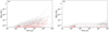Fig. 2

Mass growth of planetesimals for planets on coplanar orbits (left panel, run_md_test in Table 1) and non-coplanar orbits (right panel, run_md_1). Gray lines trace the mass of each planetesimal. Red dots represent the merging of two bodies, marked at the position of the less massive body. The early sudden growth is caused by planetesimal accretion and the later smooth growth by pebble accretion.

3.1 Mono-dispersed initial conditions

In this scenario we consider that all planetesimals start with an equal size (400 km in radius). Themass growth and dynamical evolution are simulated after the formation at a single site location. We conduct both simulations when the planetesimal orbits are coplanar and inclined. In the former case planetesimals are all initiated at z = 0 and, by construction, remain in the disk midplane. This (as we will see) is not realistic, but comparing the results between these two gives us important insights into key factors (e.g., planet inclination) shaping the planetesimal + pebble accretion process.

3.1.1 Effect of inclinations on growth of planetesimals

As mentioned in Sect. 2.3, the streaming instability produces in total 0.039 M_⊕ planetesimals at r_ice. In the mono-dispersed initial conditions, we assume that all planetesimals are 400 km in radius (6.7 × 10⁻⁵ M_⊕ in mass). Therefore, N = 580 planetesimals are generated in this compact ring belt (Δr = ηr in width). These bodies are injected into the simulation one by one after each 0.1 orbital period. Their initial semimajor axes are uniformly distributed from r_ice − Δr∕2 to r_ice + Δr∕2. The initial eccentricities are assumed to follow a Rayleigh distribution, $p (e) = e / e_{0} \exp [- e^{2} / 2 e_{0}^{2}]$ $p(e) \,{=}\, e/e_0 \exp [- e^2/2e_0^2]$ .

We conducted two sets of simulations. The first idealised set considers that planetesimals are in coplanar orbits (i_p = 0, run_md_test in Table 1). However, this configuration (i₀ = 0) is an unphysical case. Realistically, although the initial inclinations are tiny, they are not zero due to the stochastic fluctuation driven by the disk turbulence (Ida & Lin 2008; Gressel et al. 2011; Yang et al. 2012; Okuzumi & Ormel 2013). The planetesimals would be lifted out of the midplane and acquire an inclination distribution.

In hydrodynamic simulations (Simon et al. 2016; Schäfer et al. 2017) the planetesimals are generated from pebble filaments, their random fluctuation is at least smaller compared to the size of the filament (e₀, i₀ ≪ η). Therefore, for the second set we assume that their inclinations also follow a Rayleigh distribution with i₀ = e₀∕2. Two different initial values for e₀ are numerically tested, 10⁻⁵ and 10⁻⁶. We find that since the orbits of planetesimals are readily excited, the results are insensitive to the initial values. In this non-coplanar configuration, three different simulations are performed with the randomized initial semimajor axes and orbital phase angles (run_md_1 to run_md_3 in Table 1).

Figure 2 shows the mass growth of planetesimals when they are in co-planar orbits (panel a) and inclined orbits (panel b). We clearly find that mergers (red dots) occur more frequently when the orbits of the planetesimals are coplanar. In Fig. 2a the mass growth is dominated by planetesimal-planetesmial collision at the beginning (the sudden jump in mass of grey lines in Fig. 2). Since the pebble accretion rate is an increasing function of the planet mass, when the mass approaches 10⁻² M_⊕, the growth is driven by pebble accretion (smooth growth in mass in Fig. 2). Only a few bodies survive after 1 Myr, and the mass of the dominant body is 4 M_⊕. Even though the accretion timescale in this configuration is artificially short, it clearly illustrates that the growth initially proceeds in a planetesimal accretion-dominated phase (phase A) and transitions to a rapid pebble accretion dominated phase (phase B) when a massive body of ~ 10⁻³ M_⊕ to 10⁻² M_⊕ emerges. For the realistic case when planetesimals are on inclined orbits (Fig. 2b), however, much fewer mergers occur and the mass growth remains modest. The mass of the largest body remains < 10⁻² M_⊕, and there is no efficient pebble accretion at the end of the simulation.

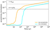Fig. 3

Root-mean-square (rms) eccentricity (orange) and inclination (cyan) of planetesimals as functions of time in run_md_1.The dashed line indicates the separation between the shear-dominated and dispersion-dominated regime, e = v_H ∕v_K. The dotted line indicates the inclination equal to the aspect ratio of the pebble disk.

Table 1

Simulations set-up in Sects. 3.1–3.3.

3.1.2 Excitation of eccentricities and inclinations

Figure 3 shows the time evolution of the root mean square (rms) of the planetesimals’ eccentricities (orange) and inclinations (cyan) in run_md_1. After a few orbits the eccentricities are quickly excited while the inclinations still remain low. This behavior occurs in the shear-dominated regime, when the velocity dispersion (δv) of planetesimals is smaller than their Hill velocity (v_H = R_HΩ_K; Ida 1990), where the mutual Hill radius 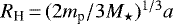$R_{H} = {(2 m_{p} / 3 M_{⋆})}^{1 / 3} a$ $R_{\textrm{H}} \,{=}\, (2m_{\textrm{p}}/3M_{\star})^{1/3} a$ . After a few hundred years their eccentricities get excited to values larger than the Hill velocity (δv > v_H, dashed line in Fig. 3), the scattering transitions to the isotropic, dispersion-dominated regime. In that case the rms inclination excites to a value equal to half of the eccentricity, i_rms ≃ e_rms∕2 (Ida et al. 1993).

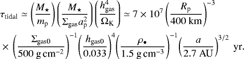
Based on the disk model, we calculate the excitation and damping timescale of the velocity dispersion of the planetesimals. The timescale of the viscous stirring (eccentricity excitation) is given by (Ida 1990; Kokubo & Ida 2000), $\begin{array}{l} τ_{vs} & ≃ & 3 \times 10^{5} (\frac{i}{0.005}) {[{(\frac{e}{0.01})}^{2} + {(\frac{i}{0.005})}^{2}]}^{\frac{3}{2}} {(\frac{R_{p}}{400 km})}^{- 3} \\ \times {(\frac{Σ_{p}}{10 g {cm}^{- 2}})}^{- 1} {(\frac{ρ_{•}}{1.5 g {cm}^{- 3}})}^{- 1} {(\frac{a}{2.7 AU})}^{- 1 / 2} yr . \end{array}$ $\begin{eqnarray*} \tau_{\textrm{vs}} &\simeq & 3 \times 10^{5} \left( \frac{i}{0.005} \right) \left[ \left(\frac{e}{0.01} \right)^2 + \left( \frac{i}{0.005} \right)^2 \right]^{\frac{3}{2}} \left( \frac{R_{\textrm{p}}}{400 \ \rm km} \right)^{-3} \nonumber\\ &&\times\,\left( \frac{\Sigma_{\textrm{p}}}{10 \textrm{\ g\,cm}^{-2}} \right)^{-1} \left( \frac{\rho_{\bullet}}{1.5 \textrm{\ g\,cm}^{-3}} \right)^{-1} \left( \frac{a}{2.7 \ \textrm{AU}} \right)^{-1/2} \ \textrm{yr}.\end{eqnarray*}$ (13)

The damping timescale of eccentricity from the gas drag is (Adachi et al. 1976), $\begin{array}{l} τ_{drag} & ≃ & 10^{7} (\frac{R_{p}}{400 km}) {(\frac{Σ_{gas0}}{500 g {cm}^{- 2}})}^{- 1} (\frac{h_{gas0}}{0.033}) \\ \times {[{(\frac{e}{10^{- 2}})}^{2} + {(\frac{i}{5 \times 10^{- 3}})}^{2} + {(\frac{η}{2.5 \times 10^{- 3}})}^{2}]}^{- 1 / 2} \\ \times (\frac{ρ_{•}}{1.5 g {cm}^{- 3}}) {(\frac{a}{2.7 AU})}^{11 / 4} yr . \end{array}$ $\begin{eqnarray*} \tau_{\textrm{drag}} &\simeq & 10^{7} \left( \frac{R_{\textrm{p}}}{400 \ \textrm{km}} \right) \left( \frac{\Sigma_{\textrm{gas0}}}{500 \textrm{\ g\,cm}^{-2}} \right)^{-1} \left( \frac{h_{\textrm{gas0}}}{0.033} \right) \nonumber\\ && \times\,\left[ \left( \frac{e}{10^{-2}} \right)^2 +\left( \frac{i}{5 \times 10^{-3}} \right)^2 + \left( \frac{\eta}{2.5 \times 10^{-3}} \right)^2 \right]^{-1/2} \nonumber\\ & &\times\,\left( \frac{\rho_{\bullet}}{1.5 \textrm{\ g\,cm}^{-3}} \right) \left( \frac{a}{2.7 \ \textrm{AU}} \right)^{11/4} \ \textrm{yr}.\end{eqnarray*}$ (14)

This damping is inefficient for large planetesimals, and is a strongly increasing function of the semimajor axis of the planet a. Tidal interactions (type I torque) between an embryo and the gas also damp its eccentricity and inclination. The damping terms are expressed as (Artymowicz 1993) $\begin{array}{l} τ_{tidal} ≃ (\frac{M_{⋆}}{m_{p}}) (\frac{M_{⋆}}{Σ_{gas} a_{p}^{2}}) (\frac{h_{gas}^{4}}{Ω_{K}}) ≃ 7 \times 10^{7} {(\frac{R_{p}}{400 km})}^{- 3} \\ \times {(\frac{Σ_{gas0}}{500 g {cm}^{- 2}})}^{- 1} {(\frac{h_{gas0}}{0.033})}^{4} {(\frac{ρ_{•}}{1.5 g {cm}^{- 3}})}^{- 1} {(\frac{a}{2.7 AU})}^{3 / 2} yr . \end{array}$ $\begin{align*} & \tau_{\textrm{tidal}} \simeq \left( \frac{M_{\star}}{ m_{\textrm{p}}} \right) \left( \frac{M_{\star}}{ \Sigma_{\textrm{gas}} a_{\textrm{p}}^2 } \right) \left( \frac{ h_{\textrm{gas}}^4 }{\Omega_{\textrm{K}}} \right) \simeq 7 \times 10^{7} \left( \frac{R_{\textrm{p}}}{400 \ \textrm{km}} \right)^{-3} \nonumber\\ & \times\,\left( \frac{\Sigma_{\textrm{gas0}}}{500 \textrm{\ g\,cm}^{-2}} \right)^{-1}\! \left( \frac{h_{\textrm{gas0}}}{0.033} \right)^4 \! \left( \frac{\rho_{\bullet}}{1.5 \textrm{\ g\,cm}^{-3}} \right)^{-1}\! \left( \frac{a}{2.7 \ \textrm{AU}} \right)^{3/2} \ \textrm{yr}.\end{align*}$ (15)

The type I damping is inversely proportional to the mass of the embryo, and is negligible when the size of the body is smaller than 1000 km (10⁻³ M_⊕). From the above equations we obtain τ_vs ≪ τ_drag < τ_tidal. We conclude that both gas drag and type I damping are ineffective to circularize the orbit of planetesimals. Their eccentricities and inclinations keep increasing with time.

The next question is why pebble accretion is inefficient in the simulation in Fig. 2b. There are two reasons. First, fewer planetesimal collisions result in less massive planetesimals. Since the pebble accretion rate correlates with the mass of the body (Eqs. (9) and (10)), less massive bodies accrete pebbles more slowly.Second, pebble accretion is quenched due to a high eccentricity and inclination. Specifically, from Eq. (11) it follows that pebble accretion requires encounters to have a sufficiently low relative velocity 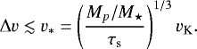$Δ v ≲ v_{*} = {(\frac{M_{p} / M_{⋆}}{τ_{s}})}^{1 / 3} v_{K} .$ $\begin{equation*}\Delta v \lesssim v_{\ast} = \left( \frac{M_p/M_{\star}}{\tau_{\textrm{s}}}\right)^{1/3} v_{\textrm{K}}. \end{equation*}$ (16)

Inserting Δv ≃ ev_K and e ~ 10⁻² we find that pebble accretion becomes only significant when the mass of the planet approaches e³ τ_sM_⋆ ≈ 10⁻²M_⊕. However, from the above discussion we know that gas drag and type I damping are ineffective to reduce the random motions of 400-km-sized planetesimals. In addition, a high planetesimal inclination further reduces pebble accretion when it becomes larger than the aspect ratio of the pebble disk (i_rms > h_peb; Levison et al. 2015). In Fig. 3 we find that this happens at t ≃ 5 × 10⁵ yr. This means after that the planetesimals exceed the pebble layer during part of its orbit, reducing the amount of pebbles they can “eat”.

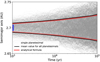Fig. 4

Orbital expansion of planetesimals as a function of time. The gray and black lines are the semimajor axis of each planetesimal and the mean value of the planetesimal population, respectively. The red line denotes the analytical expression for the width of the planetesimal belt from Eq. (17).

3.1.3 Spreading of the planetesimal belt

In Fig. 4 we plot the time evolution of the planetesimals’ semimajor axes in run_md_1. We define the full width of the planetesimal belt as $Δ W = 2 \sqrt{\sum_{i} {(a_{i} - r_{ice})}^{2} / N}$ $\Delta W \,{=}\, 2\sqrt{ \sum_{i} (a_{i} -r_{\textrm{ice}})^2/N}$ . The initial width is ηr_ice (blue area). After their injection, planetesimals in this compact zone experience mutual gravitational interactions; scatterings excite their eccentricities and, in order to conserve the angular momentum, the range of the semimajor axes also expands. In Fig. 4 we find that the width increases steadily with time and becomes 0.05 AU after 10⁵ yr.

This orbital expansion can be described by a diffusion process. Ohtsuki & Tanaka (2003) obtain an analytical expression of the viscositydue to the mutual gravitational scattering based on equally sized planetesimals. Substituting their viscosity (ν in their Eq. (18)) into $Δ W = \sqrt{ν t}$ $\Delta W \,{=}\, \sqrt{\nu t}$ , we have $Δ W = C_{w} \sqrt[3]{(N Ω_{K} t / e^{2})} R_{H}^{2} / a,$ $\begin{equation*} \Delta W = C_{\textrm{w}} \sqrt [\leftroot{-1}\uproot{2}\scriptstyle 3] {\left( N \Omega_{\textrm{K}} t /e^2 \right) } R_{\textrm{H}}^2/a,\end{equation*}$ (17)

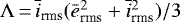where the prefactor $C_{w}^{3} = C_{fit} [24 I (β) / π^{2} \ln (Λ^{2} + 1)]$ $C_{\textrm{w}}^3 \,{=}\, C_{\textrm{fit}} [24 { I(\beta)/\pi^2\ln(\Lambda ^2 + 1)]}$ , I(β) = 0.2, t is the time, $Λ = {\bar{i}}_{rms} ({\bar{e}}_{rms}^{2} + {\bar{i}}_{rms}^{2}) / 3$ $\Lambda\,{=}\, \bar{i}_{\textrm{rms}}( \bar{e}_{\textrm{rms}}^2 + \bar{i}_{\textrm{rms}}^2)/3$ , and ī_rms = ai_rms∕R_H and ē_rms = ae_rms∕R_H. The numerical factor of C_fit = 30 is calibrated with our numerical simulations and is approximately three times larger than Ohtsuki & Tanaka (2003)’s result. This formula is obtained under the assumption that planetesimals are in the dispersion-dominated accretion regime. We show in Fig. 4 that our analytical expression (Eq. (17)) agrees well with the simulation (black line). For fixed total mass Nm_p and a, ΔW increases with time ( ∝ t^1∕3), the initial size of the planetesimal (∝ R₀), and decreases with the eccentricity (e^−2∕3).

Since the ring belt expands over time, the surface density of the planetesimal also decreases. Therefore, the accretion of the planetesimals formed from a narrow ring will be longer than the classical runaway and oligarchic accretion that assumes an “infinite” width of the planetesimal disk (Kokubo & Ida 2000).

It is clearly seen from Fig. 2b that the growth of planetesimals is slower than Fig. 2a when considering the non-zero inclinations. We find that the runs in Table 1 with different initial randomness have a similar growth trend. The masses of the most massive planetesimals from run_md_1 to run_md_3 are all far below an Earth mass.

In conclusion, when starting from a narrow ring belt of 400-km-sized planetesimals, the growth of planetesimals is suppressed by the self-excitation of the planetesimals. Planetesimal accretion is slow and pebble accretion is inefficient. Formation of planeterary embryos, let alone super-Earth planets, is impossible in this scenario, even though 100 M_⊕ of pebbles drift through.

3.2 Poly-dispersed initial conditions with large planetesimals

In the previous section we found that when the sizes of planetesimals are all 400 km, their growthis inefficient at the ice line. Then the question is: what is the realistic size of the planetesimals? In this section we consider a poly-dispersed population of planetesimals from the streaming instability simulations. In this case, planetesimals evolve into two-component mass distribution (one large embryo + small planetesimals). The large body is able to start rapid pebble accretion to eventually grow into a massive planet.

The initial mass function of planetesimals by the streaming instability has been investigated by numerous authors in detail. Simon et al. (2016, 2017) find that the initial size can be described by a single power law. Recently Schäfer et al. (2017) suggest thatthis initial mass distribution is better fitted by a power law plus a shallow exponential decay. The power law is for low- and intermediate-sized planetesimals, while the exponential decay tail represents the high mass cutoff of planetesimals (Fig. 4 in Schäfer et al. 2017). From Schäfer et al. (2017) simulations, the number fraction of planetesimals with m_p > m is given by their Eq. (19), $\frac{N_{>} (m)}{N_{tot}} = {(\frac{m}{m_{min}})}^{- p} \exp [{(\frac{m_{min}}{m_{e}})}^{β} - {(\frac{m}{m_{e}})}^{β}] .$ $\begin{equation*} \frac{N_{>}(m)}{N_{\textrm{tot}}} \,{=}\, \left(\frac{m}{ m_{\textrm{min}}} \right)^{-p} \exp\left[ \left(\frac{m_{\textrm{min}}}{m_{\textrm{e}}} \right)^{\beta} - \left(\frac{m}{ m_{\textrm{e}} } \right)^{\beta} \right].\end{equation*}$ (18)

Following this distribution, we adopt their parameters: p = 0.6, β = 0.35. The minimum mass and exponential characteristic mass are fitting parameters, which are given as m_min = 10⁻⁶ M_⊕ (100 km), m_e = 1.6 × 10⁻⁵ M_⊕ (250 km), respectively. Figure 5 illustrates the mass distribution of planetesimals for all mass range (red + blue) and for the simulated mass branch (blue). There are in total 0.039 M_⊕ planetesimals. Here we simulate the most massive 470 bodies from this population, corresponding to two-thirds of the total mass (blue branch in Fig. 5). The simulated bodies span two order of magnitude in mass and a factor of five in size, from 200 to 1000 km. For simplicity, we neglect the lower one-third of small planetesimals. These bodies, if presented, would only modestly contribute to the planetesimal accretion and dynamical friction.

Other initial conditions are chosen to be the same as the simulation of equal 400-km-sized planetesimals (Table 1). The mass growth of all planetesimals is shown in Fig. 6a while the semimajor axis of the largest body is shown in Fig. 6b. The eccentricity (solid) and inclination (dashed) evolution of the largest body and the rms values of the planetesimals are given in Fig. 6c.

For the poly-dispersed population of planetesimals simulated here, most mass is in medium-sized planetesimals of 300–400 km in size (Fig. 5). Energy equipartition leads to a configuration in which the massive planetesimals have low random velocities while the low mass planetesimals have high random velocities (Ida 1990; Goldreich et al. 2004). Therefore, the random velocity of the massive planetesimal is lower than the rms velocity dispersion due to dynamical friction. At the beginning, the largest planetesimal (black line in Fig. 6a) can accrete more neighboring planetesimals. Since its eccentricity and inclination remain low, once the mass is beyond a few 10⁻³ M_⊕, the largest planetesimals will begin to accrete pebbles very efficiently. The mass of the largest planetesimal then increases further, rendering pebble accretion more efficient compared to lower mass planetesimals. Therefore, this massive embryo dominates the subsequent growth and dynamical evolution of the system.

Rather than stop the simulation at 1 Myr, we continued it until the most massive planet migrated into the inner 0.1 AU (the assumed location of the inner disk edge) in this illustrated run (run_pd_1). We find that the planet reaches the inner disk edge at 1.2 Myr when the mass is 3.9 M_⊕. The second largest body only grew rapidly in mass when the largest one migrated out of the ring. At the end of the simulation the second largest body is still one order of magnitude less massive than the largest one.

To conclude, the presence of ~10³ km planetesimals in a sea made up predominantly of bodies of a few hundreds of kilometers will significantly speed up planet formation. This poly-dispersed population results in a low velocity dispersion of the massive body. Both effects (high m_p and low Δv) facilitate the transition to the pebble accretion dominated phase (phase B) and promote the formation of a super-Earth planet after ≃ 1 Myr.

Fig. 5

Sum of planetesimal mass in each bin for all mass planetesimals (red + blue) and for the simulated mass branch (blue) versus the initial planetesimal mass (size) from Eq. (18). The initial mass function of planetesimals was based on streaming instability simulations with a minimum mass of 10⁻⁶ M_⊕ (100 km) and a characteristic mass of 1.6 × 10⁻⁵ M_⊕ (250 km). We separate this distribution into different mass bins.

3.3 Two-component initial conditions as a result of runaway growth of small planetesimals

As demonstrated above, a poly-dispersed population of planetesimals containing initially a few very large bodies can form planets rapidly. Such an initial planetesimal mass distribution would be a consequence of forming planetesimals directly from the streaming instability. Generally, a lower pebble surface density yields smaller planetesimals in streaming instability simulations (Johansen et al. 2015; Simon et al. 2016). For the single-site planetesimal formation scenario, the pebble density is locally enhanced at a particular disk location (e.g., the ice line). However, how strong the enhancement is is determined by complicated physical processes such as water vapor diffusion and condensation (Schoonenberg & Ormel 2017). Taking these factors and uncertainties into account, we also consider the case of an initially small planetesimal size. Nevertheless, we argue in Sect. 3.3.1 that in this circumstance runaway growth of planetesimals proceeds quickly, producing the desired two-component mass distribution that promotes the formation of massive planets.

Fig. 6

Panel a: mass growth of the planetesimals for a poly-dispersed size population of planetesimals based on the blue branch of Fig. 5. The black line represent the growth of the final most massive body and gray lines are for other planetesimals. Red dots represents the merging of two bodies, marked at the position of the less massive body. The sudden growth is caused by planetesimal accretion and the smooth growth by pebble accretion. We note that f_set approaches one when the planet is 0.01 M_⊕. Panel b: semimajor axis evolution of the final most massive body. Panel c: eccentricity (solid) and inclination (dashed) evolution where black lines represent the final most massive body and the red lines indicate rms values of the planetesimals. The simulation is from run_ pd_1.

3.3.1 Runaway growth in a narrow planetesimal belt

The characteristic runaway planetesimal accretion timescale is (Ormel et al. 2010) $\begin{array}{l} τ_{rg} & = & C_{rg} \frac{ρ_{•} R_{0}}{Σ_{p} Ω_{K}} = 10^{5} (\frac{C_{rg}}{0.1}) (\frac{R_{0}}{100 km}) \\ \times {(\frac{Σ_{p}}{10 g {cm}^{- 2}})}^{- 1} {(\frac{a}{2.7 AU})}^{3 / 2} yr, \end{array}$ $\begin{eqnarray*} \tau_{\textrm{rg}} &=& C_{\textrm{rg}} \frac{ \rho_{\bullet} R_0}{ \Sigma_{\textrm{p}} \Omega_{\textrm{K}}} = 10^{5} \left(\frac{C_{\textrm{rg}}}{0.1} \right) \left(\frac{R_0}{100 \textrm{\ km}} \right) \nonumber\\[3pt] && \times\,\left(\frac{\Sigma_{\textrm{p}}}{10 \textrm{\ g\,cm}^{-2}} \right)^{-1} \left(\frac{a}{ 2.7 \ \textrm{AU} } \right)^{3/2 } \ \textrm{yr},\end{eqnarray*}$ (19)

where C_rg ≃ 0.1 is a numerical-corrected prefactor from Ormel et al. (2010), and ρ_• = 1.5 g cm⁻³ is the internal density of the planetesimal. Small planetesimals have three advantages in terms of mass growth. First, based on Eq. (19) the runaway growth timescale is proportional to the initial size of the planetesimals (R₀). It takes less time to form a runaway body (before the onset of the oligarchic growth) when starting with smaller planetesimals. Second, the eccentricity and inclination excitation by self-stirring is less severe for smaller planetesimals (Eq. (13)), which also boosts the planetesimal and pebble accretion. Third, as shown in Sect. 3.1.3, the spreading of their semimajor axes increases with the size of the planetesimal (R₀ ∝ R_H in Eq. (17)). For the same total planetesimal mass, smaller planetesimals expand their orbits less, resulting in a higher surface density. Therefore, the subsequent accretion also becomes faster.

Accounting for these effects, we assume that the planetesimals are all 100 km in size (≃10⁻⁶ M_⊕ in mass). These planetesimals would undergo a faster runaway growth and less orbital expansion compared to 400-km-sized bodies. Since the runaway growth will result in a steep mass distribution ( $d N / d m_{p} \propto m_{p}^{- 2.5}$ $\textrm{d} N/\textrm{d}m_{\textrm{p}} \propto m_{\textrm{p}}^{-2.5}$ ; Wetherill & Stewart 1993; Kokubo & Ida 1996, 2000; Ormel et al. 2010; Morishima et al. 2008), most of the mass remains in small planetesimals. As discussed in Sect. 3.2, the inclination and eccentricity of the large body could therefore be damped by small planetesimals through dynamical friction. The planet can accrete more pebbles when the orbit remains nearly coplanar and circular.

The key difference between the classical runaway and oligarchic growth scenario and our scenario is that we here consider planetesimal formation at a single location. In this study we propose a clean and simplistic physical picture. The hypothesis is that after the planetesimal runaway growth phase, the system can be well described by two components: a single big embryo of radius ~ 10³ km and a swarm of 100 km size planetesimals, which dominate the total mass. We reasonably neglect bodies in between these two are dynamically insignificant and cannot compete with the runaway body in terms of growth (also shown in Fig. 6a). Altogether, the situation resembles the classical runaway and oligarchy transition, except that, in our case, there is only one single “oligarch”.

Why is there only one big embryo instead of multiple oligarchs? The transition from the runaway to the oligarchic growth takes place when the viscous stirring timescale τ_vs (Eq. (13)) equals the runaway timescale τ_rg (Eq. (19))². When τ_vs > τ_rg, the stirring of the random velocities is smaller compared to the accretion, which is the key feature of runaway growth. When τ_vs < τ_rg, the eccentricity growth is faster than the accretion and the growth transitions to the oligarchic regime. The transition size of the planet between two regimes is given by Eq. (11) of Ormel et al. (2010), $\begin{array}{l} R_{rg/oli} ≃ & 850 {(\frac{C_{rg}}{0.1})}^{3 / 7} {(\frac{R_{0}}{100 km})}^{3 / 7} {(\frac{a}{2.7 AU})}^{5 / 7} {(\frac{Σ_{p}}{1 g {cm}^{- 2}})}^{2 / 7} km . \end{array}$ $\begin{equation*} \begin{split} R_{\textrm{rg/oli}} \simeq\,& 850 \left(\frac{C_{\textrm{rg}}}{ 0.1}\right)^{3/7}\! \left(\frac{R_0}{ 100 \ \textrm{km}}\right)^{3/7}\! \left(\frac{a}{ 2.7 \ \textrm{AU} }\right)^{5/7}\! \left(\frac{\Sigma_{\textrm{p}}}{ 1 \,\textrm{g \,cm}^{-2}} \right)^{2/7} \textrm{km}.\end{split} \end{equation*}$ (20)

Substituting Eq. (19) into Eq. (17), we obtain that when the massive body grows into a transition radius, the planetesimal belt width is $Δ W = \sqrt{\frac{C_{rg} C_{w}^{3} R_{H}^{3}}{2 R_{0}}} .$ $\begin{equation*} \Delta W = \sqrt{ \frac{C_{\textrm{rg}} C_{\textrm{w}}^3 R_{\textrm{H}}^3}{2R_0} }.\end{equation*}$ (21)

We note that R_H is the Hill radius of the planetesimal with a size of R₀. From Σ_p = M_tot,pl∕2πaΔW and Eq. (21), we calculate that the belt width extends to ΔW = 0.029 AU and the planetesimal surface density reduces to Σ_p = 2 g cm⁻² after the runaway growth (~10⁵ yr). Substituting the above values into Eq. (20), we obtain, $\begin{array}{l} R_{rg/oli} ≃ 1000 {(\frac{C_{rg}}{0.1})}^{3 / 7} {(\frac{R_{0}}{100 km})}^{1 / 7} {(\frac{M_{tot, pl}}{0.039 M_{\oplus}})}^{2 / 7} km . \end{array}$ $\begin{equation*} \begin{split} R_{\textrm{rg/oli}} \simeq 1000 \left(\frac{C_{\textrm{rg}}}{ 0.1}\right)^{3/7} \left(\frac{R_0}{ 100 \ \textrm{km}}\right)^{1/7} \left(\frac{M_{\textrm{tot,pl}}}{ 0.039 \ M_{\oplus}}\right)^{2/7} \ \textrm{km}.\end{split} \end{equation*}$ (22)

We therefore conclude that the feeding zone of this embryo (≃ 10 R_H, Kokubo & Ida 1998) is similar to the width of the planetesimal belt, supporting the one single embryo assumption.

3.3.2 Superparticle approach

Since the total planetesimal mass is 0.039 M_⊕ and small planetesimals dominate the mass, there are in total 35 000 100-km-sized planetesimals (≃ 10⁻⁶ M_⊕) in this case. It is prohibitive computationally to simulate the interactions among all these bodies with an N-body scheme. Therefore, we adopt the superparticle approach to mimic the dynamics of small bodies (see Levison et al. 2015; Raymond et al. 2016 and references therein), in which N_sp small planetesimals are clustered as one superparticle. The superparticle still feels the aerodynamical gas drag as if it were a single 100-km-sized planetesimal, but the mass of the particle is N_sp times higher(m_sp = N_spm₀). These superparticles gravitationally interact with the embryo but not with each other. This is based on the fact that the collision timescale among small planetesimals is much longer than the embryo-planetesimal collision. In principle, the approach requires m₀ ≪ m_sp ≪ m_p, where m_p is the embryo’s mass. The latter inequality is needed to ensure that dynamical friction operates correctly. The simulation would be very time-consuming for a too small N_sp, while the dynamical evolution may become artificially stochastic for a too large N_sp (low number of superparticles).

We hereassume that the velocity dispersion of small planetesimals is excited by the planetesimals themselves, and that it is close to their escape velocity ( $δ v ≃ v_{esc} = \sqrt{2 G m_{0} / R_{0}}$ $\delta v \simeq v_{\textrm{esc}} \,{=}\, \sqrt{2G m_0/R_0}$ ), that is, e ≃ e_esc = v_esc∕v_K. The eccentricities and inclinations are adopted to follow the Rayleigh distributions, where e₀ = 2i₀ = e_esc. Their semimajor axes are randomly initialized from r_ice(1 − η∕2) to r_ice(1 + η∕2). In addition, since pebble accretion is extremely inefficient for 100 km-sized planetesimals (the inequality (Eq. (16)) is far from satisfied), it is reasonable to neglect pebble accretion of the superparticles. The embryo is initially placed at r_ice.

3.3.3 Results

We have conducted simulations with different masses of the superparticle, N_sp = 25 and 50, respectively. The results are in good agreement with each other (see Section Appendix for details). The results presented in Sects. 3.3.3 and 3.3.4 are based on the N_sp = 50 run.

The disk and pebble parameters in this (run_sp) were taken to be identical torun_pd in Sect. 3.2. The mass of the embryo was chosen to be the transition value (m_p = 10⁻³ M_⊕ when R_p = R_rg/oli in Eq. (22)). Three individual simulations (run_sp_1 to run_sp_3) were conducted, varying only the initial positions and orbital phase angles of the planetesimals. In addition, we also conducted a separate simulation for the growth of a single embryo without small planetesimals. This comparison enables us to isolatethe effect of N-body dynamics (planetesimal accretion). Simulations are terminated when t = 1 Myr.

Figure 7 shows the mass growth and orbital evolution of the embryos in panels a and b, respectively. For the superparticle approach, the thick red lines represent the mean values averaging three runs (e.g., $\bar{m} (t) = \sum_{i = 1}^{3} m_{i} (t) / 3$ ${\bar m} (t) \,{=}\,\sum_{i\,{=}\,1}^{3} m_{\textrm{i}}(t)/3$ ), whereas the light red areas represent the spreading over these runs. It can be seen that the difference in mass and semimajor axis between the three simulations is small. The black dashed line represents the growth of a single embryo (assuming it is on a circular and coplanar orbit) purely by pebble accretion. We find that when starting with the transition size embryo, the planetesimal accretion is already modest and the mass growth is mainly driven by pebble accretion.

When the mass of the embryo is beyond 0.1 M_⊕, type I migration becomes important. The planet would take ~ 0.5 Myr to migrate into the inner region of the disk. Eventually, a 1.3 M_⊕ planet formswithin 1 Myr.

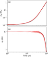Fig. 7

Panel a: mass growth of the embryo for the two-component initial conditions in run_ sp. Panel b: semimajor axis evolution of the embryo. The red thick line is for the averaged value and the light red is for the spreading over three different runs. The black dashed line is for the growth of a single embryo on a circular and coplanar orbit without any planetesimal accretion.

3.3.4 Timescale analysis

In this section we analyse the growth timescale of the embryo. The pebble accretion timescale in the 2D regime is given by $\begin{array}{l} τ_{PA, 2D} & = & \frac{m_{p}}{ε_{PA, 2D} {\dot{M}}_{peb}} ≃ 9 \times 10^{4} f_{set}^{- 1} {(\frac{m_{p}}{0.05 M_{\oplus}})}^{1 / 3} \\ \times {(\frac{τ_{s}}{0.1})}^{1 / 3} (\frac{η}{2.5 \times 10^{- 3}}) {(\frac{{\dot{M}}_{peb}}{100 M_{\oplus} {Myr}^{- 1}})}^{- 1} yr, \end{array}$ $\begin{eqnarray*} \hspace*{-6pt} \tau_{\textrm{PA,2D}} &=& \frac{m_{\textrm{p}}}{ \varepsilon_{\textrm{PA,2D}} \dot M_{\textrm{peb}}} \simeq 9 \times 10^{4} f_{\mathrm{set}}^{-1} \left(\frac{ m_{\textrm{p}}}{0.05 \ M_{\oplus}} \right)^{1/3} \nonumber\\[3pt] \hspace*{-6pt}&&\times\,\left(\frac{ \tau_{\textrm{s}}}{0.1} \right)^{1/3} \left(\frac{\eta}{2.5 \times 10^{-3}} \right) \left(\frac{\dot M_{\textrm{peb}}}{ 100 \ {M}_{\oplus}\,\textrm{Myr}^{-1}}\right)^{-1} \textrm{\ yr},\end{eqnarray*}$ (23)

where we use Eq. (9) and Δv is assumed to be dominated by the Keplerian shear since the eccentricity of the embryo is insignificant due to dynamical friction. From Eq. (11) the above f_set evaluates as $f_{set} = \exp [- 0.07 {(\frac{η}{2.5 \times 10^{- 3}})}^{2} {(\frac{m_{p}}{0.01 M_{\oplus}})}^{- 2 / 3} {(\frac{τ_{s}}{0.1})}^{2 / 3}] .$ $\begin{eqnarray*} f_{\mathrm{set}} = \exp{\left[-0.07 \left(\frac{\eta}{2.5\times 10^{-3}} \right)^2 \left(\frac{m_{\textrm{p}}}{0.01 \ M_{\oplus}} \right)^{-2/3}\! \left(\frac{ \tau_{\textrm{s}}}{0.1} \right) ^{2/3} \right]}.\vspace*{2pt}\end{eqnarray*}$ (24)

When the planet is ≳10⁻² M_⊕, f_set ≃ 1. From Eq. (24), we clearly see that f_set becomes smaller when a planet is less massive or its pebble-planet relative velocity is higher.

Similarly, in the 3D limit (Eq. (10)), the pebble accretion timescale becomes $\begin{array}{l} τ_{PA, 3D} & = & \frac{m_{p}}{ε_{PA, 3D} {\dot{M}}_{peb}} ≃ 9 \times 10^{4} f_{set}^{- 2} (\frac{h_{peb}}{4.2 \times 10^{- 3}}) \\ \times (\frac{η}{2.5 \times 10^{- 3}}) {(\frac{{\dot{M}}_{peb}}{100 M_{\oplus} {Myr}^{- 1}})}^{- 1} yr . \end{array}$ $\begin{eqnarray*} \hspace*{-5pt} \tau_{\textrm{PA,3D}} &=& \frac{m_{\textrm{p}}}{ \varepsilon_{\textrm{PA,3D}} \dot M_{\textrm{peb}}} \simeq 9 \times 10^{4} f_{\mathrm{set}}^{-2} \left(\frac{ h_{\textrm{peb}}}{ 4.2 \times 10^{-3}} \right) \nonumber\\[3pt] \hspace*{-5pt}&&\times\,\left(\frac{\eta}{2.5 \times 10^{-3}} \right) \left(\frac{\dot M_{\textrm{peb}}}{ 100 {M}_{\oplus}\,\textrm{Myr}^{-1}}\right)^{-1} \textrm{\ yr}.\end{eqnarray*}$ (25)

From the planet mass dependence in Eqs. (23) and (25), we know that the pebble accretion is in 3D when the planet mass is low, and it transitions to 2D accretion when the planet becomes more massive. The transition mass between 2D and 3D is ≃ 0.05 M_⊕ for the adopted parameters.

In order to numerically capture the transition from the planetesimal dominated accretion to the pebble dominated accretion (phase A to phase B), we conduct the superparticle approach simulations starting with a less massive embryo (m_p = 3 × 10⁻⁴ M_⊕) here. The other conditions are the same as run_sp in Table 1. Again, three individual superparticle approach simulations are performed with randomly varied initial positions and orbital phase angles of the planetesimals.

These timescale are shown in Fig. 8, where the gray, blue, light blue, and magenta lines represent growth timescales obtained from the simulation, and the pebble accretion in 3D (with and without f_set) and in 2D, respectively.We can identify the following different growth stages.

When the mass of the embryo is lower than ~10⁻³ M_⊕, the mass growth is dominated by planetesimal accretion (phase A). In this phase the growth time is relatively long, and decreases with the growing mass of the big body. Since the timescale calculation is affected by the stochasticity of the collisions, the average value over three different runs (gray line) is given in Fig. 8. The pebble accretion is inefficient in this phase because of the embryo’s low mass (small m_p in Eq. (25)) and hence the weak setting accretion (small $f_{set}^{2}$ $f_{\textrm{set}}^2$ in Eq. (25)). When the mass of the embryo becomes larger, 3D pebble accretion is more efficient than planetesimal accretion (phase B). The transition mass from the planetesimal accretion dominated regime to the pebble accretion dominated regime is close to 10⁻³ M_⊕. With increasing mass f_set increases. When f_set approaches unity, the growth timescale becomes independent of the planet mass (see Eq. (25) and the light blue in Fig. 8). Finally, growth enters the 2D pebble accretion regime when the mass approaches 0.1 M_⊕. In that case, the growth timescale starts to increase, $τ_{PA, 2D} \propto m_{p}^{1 / 3}$ $\tau_{\textrm{PA,2D}} \propto m_{\textrm{p}}^{1/3}$ (magenta line in Fig. 8), since ε_PA,2D no longer scales linearly with the planet mass.

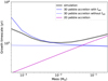Fig. 8

Growth timescale as a function of the embryo’s mass. The gray line represents the simulation whereas the blue and magenta lines are timescales for the analytical 3D and 2D pebble accretion. The dark (light) blue line corresponds to τ_3D including (orexcluding) the f_set factor (Eq. (25)).

3.4 Discussion

Comparing the cases of initial 100-km-sized and 400-km-sized planetesimals, our result suggests that starting with smaller planetesimals is more optimal for forming planets. The reason is as follows: (1) the runaway body’s size is insensitive to the initial planetesimal size ( $R_{rg/oli} \propto R_{0}^{1 / 7}$ $R_{\textrm{rg/oli}} \propto R_0^{1/7}$ , Eq. (22)) and (2) since the orbital expansion is less significant for smaller planetesimals (ΔW ∝ R₀ from Eq. (21)) and Σ_p ∝ ΔW⁻¹, the runaway accretion timescale is strongly correlated with the initial size ( $t_{rg} \propto R_{0}^{2}$ $t_{\textrm{rg}} \propto R_0^2$ from Eq. (19)). For the mono-dispersed population of 400-km-sized planetesimals, planet growth fails mainly because it takes too long to evolve into a two-component mass distribution. However, in the case of 100-km-sized planetesimals, this configuration can be realized within a fraction of the disk lifetime. In that case, the eccentricity and inclination of the large embryo remains low due to the dynamical friction of small planetesimals. It is therefore possible for the largest embryo to accrete pebbles efficiently and grow into an Earth-mass planet. As a result, massive planets could form from planetesimals with a smaller initial size.

The above discussed preferable size of the planetesimal (R₀) to grow protoplanets is dependent on the formation location of planetesimals. When the planetesimals form further out, from Eq. (19) the runaway planetesimal growth timescale increases. On the other hand, the starting size of the embryo for efficient pebble accretion also increases with the distance (Visser & Ormel 2016). This is because f_set becomes smaller when η increases with r. Therefore, both effects further limit the growth of protoplanets from a large-sized planetesimal (e.g., 400 km) when the planetesimal formation occurs at a large distance.

Our findings are similar to Levison et al. (2015). They report that large core formation by pebble accretion is only feasible after a period of classical planetesimal runaway growth. The system then ends up with a few large embryos and a swarm of small planetesimals. The embryos stir the random velocities of all small planetesimals, preventing any further growth by pebble accretion. In their case, planetesimals were born over the entire disk region and assumed to follow the same power law as the disk gas, which is based on the classical planet formation scenario (e.g., Ida & Lin 2004; Mordasini et al. 2009). The key difference with this work is that we only consider the planetesimals to form at a single site disk location with a narrow radial width. Nevertheless, the common ground between both works is that a two-component mass distribution for planetesimals is essential to promote further growth from planetesimals into protoplanets.

4 Growth and migration in the pebble accretion dominated regime

In this section, we particularly focus on growth in the pebble accretion dominated regime (phase B). We start the mass of the embryo from 10⁻³ M_⊕. As illustrated in Fig. 7, the pebble accretion dominates the growth and the planetesimals’ contribution can be neglected after m_p ≳ 10⁻³ M_⊕. The relative velocity of the massive embryo is very low due to the dynamical friction by small planetesimals and later on type I tidal damping when it grows larger. It is therefore justified to assume the embryo is on a circular and coplanar orbit. We conduct simulations for a single embryo and neglect all planetesimals, investigating the role of various disk and pebble parameters as shown in Table 2. Simulations are terminated when the planet has migrated inside of 0.1 AU.

In Table 2, the fiducial run (run_fid) is adopted to be the same disk and pebble values as in the previous sections. From run_nmig to run_lpeb, only one parameter is varied compared to the fiducial run_fid. For instance, in run_nmig we assume the planet is at the zero-torque location, where ȧ ∕a = 0. In this case, the planet does not undergo type I migration. Therefore, the planet accretes materials in situ at the ice line. From a comparison between run_nmig and run_fid, we will gain a knowledge of the effect of migration on the growth of the planet. For this purpose, we stop run_nmig at the same time when the planet in run_fid migrates inside of 0.1 AU. From a comparison between run_fid and the other individual runs (run_alpha, run_tau, run_hpeb, run_lpeb), we can understand the effect of disk turbulence, pebble size, and pebble mass flux on the planet growth.

We find in Fig. 9 that in a low turbulent disk (run_alpha, magenta) and in a disk with high pebble flux (run_hpeb, thick red), the mass growth is faster than the fiducial disk (red). In these two circumstances the planets reach 4.1 M_⊕ and 6.8 M_⊕, respectively, when they migrate inside of 0.1 AU within 1 Myr. We find the mass growth in run_nmig is very similar to the fiducial run but slightly less efficient. At t = 1.2 Myr, the final planet mass is 4.0 M_⊕ in run_fid while in run_nmig the planet always stays at the ice line and attains 3.8 M_⊕. It is also clearly seen that when the pebble flux is lower (run_lpeb, light red), or the Stokes number is lower (run_tau, orange), the mass growth is slower than the fiducial run. The protoplanet with m_p ≳ 1 M_⊕ does not form within 1 Myr from these two configurations. In run_tau the planet attains 4.8 M_⊕ when it arrives at the inner edge of the disk at t = 1.5 Myr, while in run_lpeb it grows into a 2.3 M_⊕ planet at t = 2.1 Myr.

The planet grows much faster in a high pebble flux disk. The effect of pebble mass flux on planet growth is intuitive since pebble accretion benefits from a high pebble flux (a massive pebble disk). When the planet reaches 6.8 M_⊕ and migrates into the inner disk cavity at t = 0.7 Myr in run_hpeb, the planet mass is only 0.02 M_⊕ in run_lpeb. We find a super linear correlation between the planet mass (m_p) and the integrated pebble flux (Ṁ_pebt). A factor of four in Ṁ_pebt results in more than two order of magnitude growth in M_p. This is due to the fact that pebble accretion efficiency (ε_PA) increases with m_p in both the 2D and 3D regime. The planet can initially accrete more pebbles in a high pebble flux disk. It becomes more massive due to this faster growth and would further accrete even a higher fraction of pebbles. This positive feedback promotes the rapid growth of the planet in a high pebble flux disk.

When the disk turbulence is lower, the pebble scale height becomes smaller (Eq. (8)). The transition mass from 3D to 2D pebble accretion will also become lower. Therefore, in run_alpha the embryo starts efficient 2D pebble accretion earlier than the fiducial run. Eventually, it takes less time to grow into a super-Earth planet in a lower turbulent disk.

The Stokes number has an opposite effect to the turbulent α_t in terms of thepebble scale height. Lower Stokes number pebbles mean they are more tightly coupled to the gas, and the pebble scale height becomes larger. Therefore, from Eqs. (23) and (25) transition mass from 3D to 2D in run_tau is 0.15 M_⊕, three times higher than the fiducial run. In this case starting with 10⁻³ M_⊕, the planet grows a significant fraction of its mass in the slow, 3D pebble accretion regime. On the other hand, when the planet enters 2D pebble accretion, the accretion is faster when the Stokes number is lower (Eq. (23)). Balancing these two effects, we find that the planet growth is slightly slower in run_tau compared to the fiducial run.

The effect of pebble mass flux on the planet growth is super linear. A high pebble disk mass benefits the formation of a massive planet. A less turbulent disk and large Stokes number pebbles also promote pebble accretion and the formation of a massive planet.

Table 2

Simulations for the parameter study in Sect. 4.

5 Summary

Streaming instability is an important mechanism to convert pebbles into planetesimals. It occurs at the location in the disk where the pebble density is locally enhanced (e.g., the ice line). In this work, we have focused on the growth of the planetesimals after they have formed by this mechanism at a single site disk location.

This annular (ring) planetesimal formation scenario differs from the classical planetesimal accretion scenario in two ways. First, streaming instability generates planetesimals in a narrow ring at a specific location. Most of the mass is in the largest planetesimals of a few hundred kilometers in size. In contrast, in the classical scenario planetesimals form everywhere in the disk, for example, typically following the surface density distribution of the gas. In simulations their planetesimal surface density remains constant by supplying material from the neighboring region (Kokubo & Ida 2000). This means that the orbital spreading is unimportant, in contrast to the ring formation scenario. Second, the planetesimals in our scenario grow their mass by accreting surrounding planetesimals and inwardly drifting pebbles. The mass at which the planet transitions from accreting predominantly planetesimals to pebbles occurs at ≃ 10⁻³ M_⊕.

We have modified the Mercury N-body code to perform simulations of the mass growth and orbital evolution of these planetesimals (Sect. 2). The code includes the effects of gravitational interactions and collisions among planets and planetesimals, planet–disk interactions (gas drag and type I torque), pebble accretion based on the calculation of Liu & Ormel (2018) and Ormel & Liu (2018) that accounts for the disk parameters (τ_s, η, α and Ṁ_peb), and planet properties (m_p, a, e, i). Simulations with different initial planetesimal sizes and disk parameters are investigated.

The key findings of this study are the following:

1.
Protoplanets cannot emerge from a mono-dispersed population of 400 km-sizedplanetesimals, fuelled by a 100 M_⊕ reservoir of pebbles in the outer disk. Although the initial eccentricities and inclinations are very tiny, they soon get excited through gravitational scatterings. Mechanisms such as gas drag and type I damping are not sufficient to damp their random velocities. Both planetesimal and pebble accretion are strongly suppressed when inclinations and eccentricities of planetesimals become moderate. In this circumstance, the growth of the planetesimals is mainly in the slow planetesimal accretion dominated phase (Sect. 3.1).
2.
Protoplanets can form when streaming instability has in addition spawned a population of larger planetesimals. The largest body grows by planetesimal accretion. Soon after it approaches 10⁻² M_⊕, the growth enters the rapid pebble accretion dominated regime. During this time the random velocity of the largest body remains low through the dynamical friction of small planetesimals. Finally a super-Earth planet can form within 1 Myr (Sect. 3.2).
3.
Alternatively, protoplanets also form out of their birth ring when the initial size of the planetesimals is small (e.g., 100 km). These small planetesimals are expected to undergo a runaway planetesimal accretion to form a massive embryo rapidly. In this way, the two-component mass distribution is also achieved. We find that an Earth-mass planet can form as well (Sect. 3.3)
4.
Planets grow larger when the pebble mass flux is higher, the disk is less turbulent, and the Stokes number of pebbles is larger. In particular, the growth of the planet mass increases super linearly with the disk pebble mass flux (Sect. 4).

Planetesimal accretion and pebble accretion are not two isolated processes in planet formation. From the streaming instability point of view, pebbles are converted into planetesimals, whereafter these planetesimals accrete nearby planetesimals and pebbles at the same time. The total amount of solids in disks is either in small pebbles, or in large planets or planetesimals. Therefore, a certain level of competition exists between planetesimal formation and planet growth by pebble accretion.

In addition, this work only considered the case of a single burst of planetesimal formation by streaming instability. In reality, even at the ice line the streaming instability may be triggered multiple times (episodic bursts) during the gas disk lifetime, because the planets migrate out of their birth ring. Protoplanets then emerge sequentially and a chain of multiple planets forms, as envisioned by Ormel et al. (2017).

To address these issues, a global disk model is needed. Using a novel Lagrangian approach, such a model has just been developed (Schoonenberg et al. 2018). Because of the flexibility of the Lagrangian (particle-oriented) model, it is straightforward to couple it to the N-body model presented in this paper. Such a model can then, potentially, simulate planet formation in its entirety – starting from dust coagulation and ending with a planetary architecture. It can be applied to model “complete” (as far as one can tell) planetary systems, such as those discovered around TRAPPIST-1 (Gillon et al. 2017).

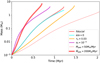Fig. 9

Mass growth of one single embryo in Sect. 3.3 for different runs given in Table 2. The red, cyan, orange, and magenta correspond to run_fid, run_nmig, run_tau, and run_alpha, respectively. The thick and thin red lines represent run_hpeb and run_lpeb.

Acknowledgements

We thank Chao-Chin Yang, Rixin Li, Carsten Dominik, and Melvyn Davies for useful discussions, and Bertram Bitsch and Djoeke Schoonenberg for proofreading the manuscript. We also thank the anonymous referee for their insightful suggestions and comments. B.L. thanks the support of the Netherlands Organization for Scientific Research (NWO; VIDI project 639.042.422), the European Research Council (ERC Consolidator Grant 724687-PLANETESYS), and the Swedish Walter Gyllenberg Foundation. C.O. is supported by the Netherlands Organization for Scientific Research (NWO; VIDI project 639.042.422). A.J. is funded by the Swedish Research Council (grant 2014-5775), the Knut and Alice Wallenberg Foundation (grants 2012.0150, 2014.0017) and the European Research Council (ERC Consolidator Grant 724687-PLANETESYS). The computations are performed on resourcesprovided by the Swedish Infrastructure for Computing (SNIC) at the LUNARC-Centre in Lund.

Appendix A Convergence test for superparticle simulations

We show the simulations with a different mass of the superparticle (m_sp = N_spm₀) for run_sp starting with m_p = 3 × 10⁻⁴ M_⊕ in Sect. 3.3.4. Three simulations with randomized initial conditions are performed for each set of N_sp. The results are shown in Fig. A.1 where red and green represent N_sp = 25 and 50, respectively.The thick line represents the mean value averaged from three individual simulations, for instance, $\bar{m} (t) = \sum_{i = 1}^{3} m_{i} (t) / 3,$ ${\bar m} (t) \,{=}\,\sum_{i\,{=}\,1}^{3} m_{\textrm{i}}(t)/3,$ whereas the light region marks the range between the minimum and maximum values from the three simulations.

Figure A.1 shows the mass, semimajor axis evolution of the embryo, and eccentricities of both planetesimals and the embryo. We find that the mass and semimajor axis converge quite well for the above two N_sp. In Fig. A.1a the difference between the mean mass for the above N_sp s is smaller compared to the spreading over individual runs (stochastic N-body effects). The excitation of planetesimals by the presence of the embryo also agrees with each other in Fig. A.1c. To summarize, results from the three N_sp tested above are in general agreement with each other.

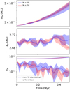Fig. A.1

Convergence test for N_sp = 25 (red) and 50 (blue). Mass, semimajor axis, and eccentricity evolution of the embryo are shown. The line represents the mean value of three individual runs while the area indicates the scattering from these runs. In the bottom panel, the RMS eccentricity of the planetesimals is shown by the dashed line.

References

Abod, C. P., Simon, J. B., Li, R., et al. 2018, ArXiv e-prints [arXiv:1810.10018] [Google Scholar]
Adachi, I., Hayashi, C., & Nakazawa, K. 1976, Prog. Theor. Phys., 56, 1756 [NASA ADS] [CrossRef] [Google Scholar]
Andrews, S. M., Wilner, D. J., Hughes, A. M., Qi, C., & Dullemond, C. P. 2009, ApJ, 700, 1502 [NASA ADS] [CrossRef] [Google Scholar]
Andrews, S. M., Rosenfeld, K. A., Kraus, A. L., & Wilner, D. J. 2013, ApJ, 771, 129 [NASA ADS] [CrossRef] [Google Scholar]
Ansdell, M., Williams, J. P., Manara, C. F., et al. 2017, AJ, 153, 240 [NASA ADS] [CrossRef] [EDP Sciences] [Google Scholar]
Artymowicz, P. 1993, ApJ, 419, 155 [NASA ADS] [CrossRef] [Google Scholar]
Ataiee, S., Baruteau, C., Alibert, Y., & Benz, W. 2018, A&A, 615, A110 [NASA ADS] [CrossRef] [EDP Sciences] [Google Scholar]
Bai, X.-N., & Stone, J. M. 2010, ApJ, 722, 1437 [NASA ADS] [CrossRef] [Google Scholar]
Baruteau, C., Crida, A., Paardekooper, S.-J., et al. 2014, Protostars and Planets VI (Tucson, AZ: University of Arizona Press), 667 [Google Scholar]
Benítez-Llambay, P., Masset, F., Koenigsberger, G., & Szulágyi, J. 2015, Nature, 520, 63 [NASA ADS] [CrossRef] [Google Scholar]
Birnstiel, T., Klahr, H., & Ercolano, B. 2012, A&A, 539, A148 [NASA ADS] [CrossRef] [EDP Sciences] [Google Scholar]
Bitsch, B., Johansen, A., Lambrechts, M., & Morbidelli, A. 2015, A&A, 575, A28 [NASA ADS] [CrossRef] [EDP Sciences] [Google Scholar]
Bitsch, B., Morbidelli, A., Johansen, A., et al. 2018, A&A, 612, A30 [NASA ADS] [CrossRef] [EDP Sciences] [Google Scholar]
Brasser, R., Bitsch, B., & Matsumura, S. 2017, AJ, 153, 222 [NASA ADS] [CrossRef] [Google Scholar]
Carrera, D., Johansen, A., & Davies, M. B. 2015, A&A, 579, A43 [NASA ADS] [CrossRef] [EDP Sciences] [Google Scholar]
Carrera, D., Gorti, U., Johansen, A., & Davies, M. B. 2017, ApJ, 839, 16 [NASA ADS] [CrossRef] [Google Scholar]
Chambers, J. E. 1999, MNRAS, 304, 793 [NASA ADS] [CrossRef] [MathSciNet] [Google Scholar]
Chatterjee, S., & Tan, J. C. 2014, ApJ, 780, 53 [NASA ADS] [CrossRef] [Google Scholar]
Chrenko, O., Brož, M., & Lambrechts, M. 2017, A&A, 606, A114 [NASA ADS] [CrossRef] [EDP Sciences] [Google Scholar]
Cresswell, P., & Nelson, R. P. 2008, A&A, 482, 677 [NASA ADS] [CrossRef] [EDP Sciences] [Google Scholar]
Dominik, C., & Tielens, A. G. G. M. 1997, ApJ, 480, 647 [NASA ADS] [CrossRef] [Google Scholar]
Dra̧żkowska, J., & Alibert, Y. 2017, A&A, 608, A92 [NASA ADS] [CrossRef] [EDP Sciences] [Google Scholar]
Flaherty, K. M., Hughes, A. M., Rosenfeld, K. A., et al. 2015, ApJ, 813, 99 [NASA ADS] [CrossRef] [Google Scholar]
Flaherty, K. M., Hughes, A. M., Rose, S. C., et al. 2017, ApJ, 843, 150 [NASA ADS] [CrossRef] [Google Scholar]
Garaud, P., & Lin, D. N. C. 2007, ApJ, 654, 606 [Google Scholar]
Gillon, M., Triaud, A. H. M. J., Demory, B.-O., et al. 2017, Nature, 542, 456 [NASA ADS] [CrossRef] [PubMed] [Google Scholar]
Goldreich, P., & Tremaine, S. 1979, ApJ, 233, 857 [NASA ADS] [CrossRef] [MathSciNet] [Google Scholar]
Goldreich, P., Lithwick, Y., & Sari, R. 2004, ARA&A, 42, 549 [NASA ADS] [CrossRef] [Google Scholar]
Greenberg, R., Wacker, J. F., Hartmann, W. K., & Chapman, C. R. 1978, Icarus, 35, 1 [NASA ADS] [CrossRef] [Google Scholar]
Gressel, O., Nelson, R. P., & Turner, N. J. 2011, MNRAS, 415, 3291 [NASA ADS] [CrossRef] [Google Scholar]
Guillot, T., Ida, S., & Ormel, C. W. 2014, A&A, 572, A72 [NASA ADS] [CrossRef] [EDP Sciences] [Google Scholar]
Güttler, C., Blum, J., Zsom, A., Ormel, C. W., & Dullemond, C. P. 2010, A&A, 513, A56 [NASA ADS] [CrossRef] [EDP Sciences] [Google Scholar]
Hansen, B. M. S. 2009, ApJ, 703, 1131 [NASA ADS] [CrossRef] [Google Scholar]
Hayashi, C. 1981, Prog. Theor. Phys. Suppl., 70, 35 [NASA ADS] [CrossRef] [MathSciNet] [Google Scholar]
Hu, X., Tan, J. C., Zhu, Z., et al. 2018, ApJ, 857, 20 [NASA ADS] [CrossRef] [Google Scholar]
Ida, S. 1990, Icarus, 88, 129 [CrossRef] [MathSciNet] [Google Scholar]
Ida, S., & Lin,D. N. C. 2004, ApJ, 604, 388 [NASA ADS] [CrossRef] [PubMed] [Google Scholar]
Ida, S., & Lin,D. N. C. 2008, ApJ, 673, 487 [NASA ADS] [CrossRef] [Google Scholar]
Ida, S., & Makino, J. 1993, Icarus, 106, 210 [NASA ADS] [CrossRef] [MathSciNet] [Google Scholar]
Ida, S., Kokubo, E., & Makino, J. 1993, MNRAS, 263, 875 [NASA ADS] [CrossRef] [Google Scholar]
Ida, S., Guillot, T., & Morbidelli, A. 2016, A&A, 591, A72 [NASA ADS] [CrossRef] [EDP Sciences] [Google Scholar]
Izidoro, A., & Raymond, S. N. 2018, in Handbook of Exoplanets, eds. H. Deeg & J. A. Belmonte (Cham, Switzerland: Springer International Publishing AG), 142 [Google Scholar]
Johansen, A., & Klahr, H. 2005, ApJ, 634, 1353 [NASA ADS] [CrossRef] [Google Scholar]
Johansen, A., & Lambrechts, M. 2017, Ann. Rev. Earth Planet. Sci., 45, 359 [NASA ADS] [CrossRef] [Google Scholar]
Johansen, A., Oishi, J. S., Mac Low, M.-M., et al. 2007, Nature, 448, 1022 [Google Scholar]
Johansen, A., Youdin, A., & Mac Low, M.-M. 2009, ApJ, 704, L75 [NASA ADS] [CrossRef] [Google Scholar]
Johansen, A., Youdin, A. N., & Lithwick, Y. 2012, A&A, 537, A125 [NASA ADS] [CrossRef] [EDP Sciences] [Google Scholar]
Johansen, A., Blum, J., Tanaka, H., et al. 2014, Protostars and Planets VI (Tucson, AZ: University of Arizona Press), 547 [Google Scholar]
Johansen, A., Mac Low, M.-M., Lacerda, P., & Bizzarro, M. 2015, Sci. Adv., 1, 1500109 [NASA ADS] [CrossRef] [Google Scholar]
Kataoka, A., Tanaka, H., Okuzumi, S., & Wada, K. 2013, A&A, 557, L4 [NASA ADS] [CrossRef] [EDP Sciences] [Google Scholar]
Kenyon, S. J.,& Bromley, B. C. 2010, ApJS, 188, 242 [NASA ADS] [CrossRef] [Google Scholar]
Kley, W., & Nelson, R. P. 2012, ARA&A, 50, 211 [NASA ADS] [CrossRef] [Google Scholar]
Kokubo, E., & Ida, S. 1996, Icarus, 123, 180 [NASA ADS] [CrossRef] [Google Scholar]
Kokubo, E., & Ida, S. 1998, Icarus, 131, 171 [NASA ADS] [CrossRef] [Google Scholar]
Kokubo, E., & Ida, S. 2000, Icarus, 143, 15 [NASA ADS] [CrossRef] [Google Scholar]
Kretke, K. A., & Lin, D. N. C. 2012, ApJ, 755, 74 [NASA ADS] [CrossRef] [Google Scholar]
Krijt, S., Ormel, C. W., Dominik, C., & Tielens, A. G. G. M. 2016, A&A, 586, A20 [NASA ADS] [CrossRef] [EDP Sciences] [Google Scholar]
Lambrechts, M., & Johansen, A. 2012, A&A, 544, A32 [Google Scholar]
Lambrechts, M., & Johansen, A. 2014, A&A, 572, A107 [NASA ADS] [CrossRef] [EDP Sciences] [Google Scholar]
Lambrechts, M., Johansen, A., & Morbidelli, A. 2014, A&A, 572, A35 [NASA ADS] [CrossRef] [EDP Sciences] [Google Scholar]
Leinhardt, Z. M., & Stewart, S. T. 2012, ApJ, 745, 79 [NASA ADS] [CrossRef] [Google Scholar]
Levison, H. F., Kretke, K. A., & Duncan, M. J. 2015, Nature, 524, 322 [CrossRef] [Google Scholar]
Li, R., Youdin, A. N., & Simon, J. B. 2018, ApJ, 862, 14 [NASA ADS] [CrossRef] [Google Scholar]
Lissauer, J. J. 1987, Icarus, 69, 249 [NASA ADS] [CrossRef] [Google Scholar]
Liu, B., & Ormel, C. W. 2018, A&A, 615, A138 [NASA ADS] [CrossRef] [EDP Sciences] [Google Scholar]
Manara, C. F., Rosotti, G., Testi, L., et al. 2016, A&A, 591, L3 [NASA ADS] [CrossRef] [EDP Sciences] [Google Scholar]
Masset, F. S. 2017, MNRAS, 472, 4204 [NASA ADS] [CrossRef] [Google Scholar]
McNally, C. P., Nelson, R. P., & Paardekooper, S.-J. 2018, MNRAS, 477, 4596 [NASA ADS] [CrossRef] [Google Scholar]
Morbidelli, A., Bottke, W. F., Nesvorný, D., & Levison, H. F. 2009, Icarus, 204, 558 [NASA ADS] [CrossRef] [Google Scholar]
Morbidelli, A., Lambrechts, M., Jacobson, S., & Bitsch, B. 2015, Icarus, 258, 418 [NASA ADS] [CrossRef] [Google Scholar]
Mordasini, C., Alibert, Y., & Benz, W. 2009, A&A, 501, 1139 [NASA ADS] [CrossRef] [EDP Sciences] [Google Scholar]
Morishima, R., Schmidt, M. W., Stadel, J., & Moore, B. 2008, ApJ, 685, 1247 [NASA ADS] [CrossRef] [Google Scholar]
Mustill, A. J., Davies, M. B., & Johansen, A. 2018, MNRAS, 478, 2896 [NASA ADS] [CrossRef] [Google Scholar]
Ohtsuki, K., & Tanaka, H. 2003, Icarus, 162, 47 [NASA ADS] [CrossRef] [Google Scholar]
Okuzumi, S., & Ormel, C. W. 2013, ApJ, 771, 43 [NASA ADS] [CrossRef] [Google Scholar]
Okuzumi, S., Tanaka, H., Kobayashi, H., & Wada, K. 2012, ApJ, 752, 106 [NASA ADS] [CrossRef] [Google Scholar]
Ormel, C. W. 2017, Astrophys. Space Sci. Lib., 445, 197 [NASA ADS] [CrossRef] [Google Scholar]
Ormel, C. W., & Klahr, H. H. 2010, A&A, 520, A43 [NASA ADS] [CrossRef] [EDP Sciences] [Google Scholar]
Ormel, C. W., & Liu, B. 2018, A&A, 615, A178 [NASA ADS] [CrossRef] [EDP Sciences] [Google Scholar]
Ormel, C. W., Dullemond, C. P., & Spaans, M. 2010, ApJ, 714, L103 [NASA ADS] [CrossRef] [Google Scholar]
Ormel, C. W., Liu, B., & Schoonenberg, D. 2017, A&A, 604, A1 [NASA ADS] [CrossRef] [EDP Sciences] [Google Scholar]
Paardekooper,S.-J. 2014, MNRAS, 444, 2031 [NASA ADS] [CrossRef] [Google Scholar]
Paardekooper,S.-J., Baruteau, C., Crida, A., & Kley, W. 2010, MNRAS, 401, 1950 [NASA ADS] [CrossRef] [Google Scholar]
Paardekooper,S.-J., Baruteau, C., & Kley, W. 2011, MNRAS, 410, 293 [NASA ADS] [CrossRef] [Google Scholar]
Pérez, L. M., Chandler, C. J., Isella, A., et al. 2015, ApJ, 813, 41 [NASA ADS] [CrossRef] [Google Scholar]
Pinte, C., Dent, W. R. F., Ménard, F., et al. 2016, ApJ, 816, 25 [NASA ADS] [CrossRef] [Google Scholar]
Rafikov, R. R. 2004, AJ, 128, 1348 [NASA ADS] [CrossRef] [Google Scholar]
Raymond, S. N., Kokubo, E., Morbidelli, A., Morishima, R., & Walsh, K. J. 2014, Protostars and Planets VI (Tucson, AZ: University of Arizona Press), 595 [Google Scholar]
Raymond, S. N., Izidoro, A., Bitsch, B., & Jacobson, S. A. 2016, MNRAS, 458, 2962 [NASA ADS] [CrossRef] [Google Scholar]
Ricci, L., Testi, L., Natta, A., et al. 2010, A&A, 512, A15 [NASA ADS] [CrossRef] [EDP Sciences] [Google Scholar]
Ros, K., & Johansen, A. 2013, A&A, 552, A137 [NASA ADS] [CrossRef] [EDP Sciences] [Google Scholar]
Schäfer, U., Yang, C.-C., & Johansen, A. 2017, A&A, 597, A69 [NASA ADS] [CrossRef] [EDP Sciences] [Google Scholar]
Schoonenberg, D., & Ormel, C. W. 2017, A&A, 602, A21 [NASA ADS] [CrossRef] [EDP Sciences] [Google Scholar]
Schoonenberg, D., Ormel, C. W., & Krijt, S. 2018, A&A, 620, A134 [NASA ADS] [CrossRef] [EDP Sciences] [Google Scholar]
Simon, J. B., Armitage, P. J., Li, R., & Youdin, A. N. 2016, ApJ, 822, 55 [NASA ADS] [CrossRef] [Google Scholar]
Simon, J. B., Armitage, P. J., Youdin, A. N., & Li, R. 2017, ApJ, 847, L12 [NASA ADS] [CrossRef] [Google Scholar]
Tazzari, M., Testi, L., Ercolano, B., et al. 2016, A&A, 588, A53 [NASA ADS] [CrossRef] [EDP Sciences] [Google Scholar]
Thommes, E. W., Duncan, M. J., & Levison, H. F. 2003, Icarus, 161, 431 [NASA ADS] [CrossRef] [MathSciNet] [Google Scholar]
Visser, R. G., & Ormel, C. W. 2016, A&A, 586, A66 [NASA ADS] [CrossRef] [EDP Sciences] [Google Scholar]
Weidenschilling, S. J. 1977, MNRAS, 180, 57 [NASA ADS] [CrossRef] [Google Scholar]
Weidenschilling, S. J. 2011, Icarus, 214, 671 [NASA ADS] [CrossRef] [Google Scholar]
Wetherill, G. W., & Stewart, G. R. 1989, Icarus, 77, 330 [NASA ADS] [CrossRef] [Google Scholar]
Wetherill, G. W., & Stewart, G. R. 1993, Icarus, 106, 190 [NASA ADS] [CrossRef] [PubMed] [Google Scholar]
Yang, C.-C., & Johansen, A. 2014, ApJ, 792, 86 [NASA ADS] [CrossRef] [Google Scholar]
Yang, C.-C., & Johansen, A. 2016, ApJS, 224, 39 [NASA ADS] [CrossRef] [Google Scholar]
Yang, C.-C., Mac Low, M.-M., & Menou, K. 2012, ApJ, 748, 79 [NASA ADS] [CrossRef] [Google Scholar]
Yang, C.-C., Johansen, A., & Carrera, D. 2017, A&A, 606, A80 [NASA ADS] [CrossRef] [EDP Sciences] [Google Scholar]
Yang, C.-C., Mac Low, M.-M., & Johansen, A. 2018, ApJ, 868, 27 [NASA ADS] [CrossRef] [Google Scholar]
Youdin, A. N., & Goodman, J. 2005, ApJ, 620, 459 [NASA ADS] [CrossRef] [Google Scholar]
Youdin, A. N., & Lithwick, Y. 2007, Icarus, 192, 588 [NASA ADS] [CrossRef] [Google Scholar]
Zhu, Z., Stone, J. M., & Bai, X.-N. 2015, ApJ, 801, 81 [NASA ADS] [CrossRef] [Google Scholar]
Zsom, A., Ormel, C. W., Güttler, C., Blum, J., & Dullemond, C. P. 2010, A&A, 513, A57 [NASA ADS] [CrossRef] [EDP Sciences] [Google Scholar]

¹

A more general form of f_set can be found in Eq. (35) of Ormel & Liu (2018), considering the pebble’s velocity distribution in a three-dimensional turbulent disk.

²

This criterion is different from Kokubo & Ida (1998). A discussion can be found in Ormel et al. (2010).

All Tables

Table 1

Simulations set-up in Sects. 3.1–3.3.

In the text

Table 2

Simulations for the parameter study in Sect. 4.

In the text

All Figures

Fig. 1

Sketch illustrating the initial setup. Planetesimals (purple circles) have formed at a single location by streaming instability. They accrete both among themselves as well as from the inward drifting pebbles (blue). The pebble disk and gas disk are marked in light blue and light green, where the gas and pebble scale heights are H_gas and H_peb, respectively. The horizontal black arrow represents the radial width (ηr) of the forming planetesimal ring. Due to dynamical friction, large planetesimals have low eccentricities and inclinations whereas small planetesimals have high velocity dispersions.

In the text

Fig. 2

Mass growth of planetesimals for planets on coplanar orbits (left panel, run_md_test in Table 1) and non-coplanar orbits (right panel, run_md_1). Gray lines trace the mass of each planetesimal. Red dots represent the merging of two bodies, marked at the position of the less massive body. The early sudden growth is caused by planetesimal accretion and the later smooth growth by pebble accretion.

In the text

	Fig. 3 Root-mean-square (rms) eccentricity (orange) and inclination (cyan) of planetesimals as functions of time in run_md_1.The dashed line indicates the separation between the shear-dominated and dispersion-dominated regime, e = v_H ∕v_K. The dotted line indicates the inclination equal to the aspect ratio of the pebble disk.
In the text

	Fig. 4 Orbital expansion of planetesimals as a function of time. The gray and black lines are the semimajor axis of each planetesimal and the mean value of the planetesimal population, respectively. The red line denotes the analytical expression for the width of the planetesimal belt from Eq. (17).
In the text

Fig. 5

Sum of planetesimal mass in each bin for all mass planetesimals (red + blue) and for the simulated mass branch (blue) versus the initial planetesimal mass (size) from Eq. (18). The initial mass function of planetesimals was based on streaming instability simulations with a minimum mass of 10⁻⁶ M_⊕ (100 km) and a characteristic mass of 1.6 × 10⁻⁵ M_⊕ (250 km). We separate this distribution into different mass bins.

In the text

Fig. 6

Panel a: mass growth of the planetesimals for a poly-dispersed size population of planetesimals based on the blue branch of Fig. 5. The black line represent the growth of the final most massive body and gray lines are for other planetesimals. Red dots represents the merging of two bodies, marked at the position of the less massive body. The sudden growth is caused by planetesimal accretion and the smooth growth by pebble accretion. We note that f_set approaches one when the planet is 0.01 M_⊕. Panel b: semimajor axis evolution of the final most massive body. Panel c: eccentricity (solid) and inclination (dashed) evolution where black lines represent the final most massive body and the red lines indicate rms values of the planetesimals. The simulation is from run_ pd_1.

In the text

	Fig. 7 Panel a: mass growth of the embryo for the two-component initial conditions in run_ sp. Panel b: semimajor axis evolution of the embryo. The red thick line is for the averaged value and the light red is for the spreading over three different runs. The black dashed line is for the growth of a single embryo on a circular and coplanar orbit without any planetesimal accretion.
In the text

	Fig. 8 Growth timescale as a function of the embryo’s mass. The gray line represents the simulation whereas the blue and magenta lines are timescales for the analytical 3D and 2D pebble accretion. The dark (light) blue line corresponds to τ_3D including (orexcluding) the f_set factor (Eq. (25)).
In the text

	Fig. 9 Mass growth of one single embryo in Sect. 3.3 for different runs given in Table 2. The red, cyan, orange, and magenta correspond to run_fid, run_nmig, run_tau, and run_alpha, respectively. The thick and thin red lines represent run_hpeb and run_lpeb.
In the text

	Fig. A.1 Convergence test for N_sp = 25 (red) and 50 (blue). Mass, semimajor axis, and eccentricity evolution of the embryo are shown. The line represents the mean value of three individual runs while the area indicates the scattering from these runs. In the bottom panel, the RMS eccentricity of the planetesimals is shown by the dashed line.
In the text

Current usage metrics show cumulative count of Article Views (full-text article views including HTML views, PDF and ePub downloads, according to the available data) and Abstracts Views on Vision4Press platform.

Data correspond to usage on the plateform after 2015. The current usage metrics is available 48-96 hours after online publication and is updated daily on week days.

Initial download of the metrics may take a while.

[1] Abod, C. P., Simon, J. B., Li, R., et al. 2018, ArXiv e-prints [arXiv:1810.10018] [Google Scholar]

[2] Adachi, I., Hayashi, C., & Nakazawa, K. 1976, Prog. Theor. Phys., 56, 1756 [NASA ADS] [CrossRef] [Google Scholar]

[3] Andrews, S. M., Wilner, D. J., Hughes, A. M., Qi, C., & Dullemond, C. P. 2009, ApJ, 700, 1502 [NASA ADS] [CrossRef] [Google Scholar]

[4] Andrews, S. M., Rosenfeld, K. A., Kraus, A. L., & Wilner, D. J. 2013, ApJ, 771, 129 [NASA ADS] [CrossRef] [Google Scholar]

[5] Ansdell, M., Williams, J. P., Manara, C. F., et al. 2017, AJ, 153, 240 [NASA ADS] [CrossRef] [EDP Sciences] [Google Scholar]

[6] Artymowicz, P. 1993, ApJ, 419, 155 [NASA ADS] [CrossRef] [Google Scholar]

[7] Ataiee, S., Baruteau, C., Alibert, Y., & Benz, W. 2018, A&A, 615, A110 [NASA ADS] [CrossRef] [EDP Sciences] [Google Scholar]

[8] Bai, X.-N., & Stone, J. M. 2010, ApJ, 722, 1437 [NASA ADS] [CrossRef] [Google Scholar]

[9] Baruteau, C., Crida, A., Paardekooper, S.-J., et al. 2014, Protostars and Planets VI (Tucson, AZ: University of Arizona Press), 667 [Google Scholar]

[10] Benítez-Llambay, P., Masset, F., Koenigsberger, G., & Szulágyi, J. 2015, Nature, 520, 63 [NASA ADS] [CrossRef] [Google Scholar]

[11] Birnstiel, T., Klahr, H., & Ercolano, B. 2012, A&A, 539, A148 [NASA ADS] [CrossRef] [EDP Sciences] [Google Scholar]

[12] Bitsch, B., Johansen, A., Lambrechts, M., & Morbidelli, A. 2015, A&A, 575, A28 [NASA ADS] [CrossRef] [EDP Sciences] [Google Scholar]

[13] Bitsch, B., Morbidelli, A., Johansen, A., et al. 2018, A&A, 612, A30 [NASA ADS] [CrossRef] [EDP Sciences] [Google Scholar]

[14] Brasser, R., Bitsch, B., & Matsumura, S. 2017, AJ, 153, 222 [NASA ADS] [CrossRef] [Google Scholar]

[15] Carrera, D., Johansen, A., & Davies, M. B. 2015, A&A, 579, A43 [NASA ADS] [CrossRef] [EDP Sciences] [Google Scholar]

[16] Carrera, D., Gorti, U., Johansen, A., & Davies, M. B. 2017, ApJ, 839, 16 [NASA ADS] [CrossRef] [Google Scholar]

[17] Chambers, J. E. 1999, MNRAS, 304, 793 [NASA ADS] [CrossRef] [MathSciNet] [Google Scholar]

[18] Chatterjee, S., & Tan, J. C. 2014, ApJ, 780, 53 [NASA ADS] [CrossRef] [Google Scholar]

[19] Chrenko, O., Brož, M., & Lambrechts, M. 2017, A&A, 606, A114 [NASA ADS] [CrossRef] [EDP Sciences] [Google Scholar]

[20] Cresswell, P., & Nelson, R. P. 2008, A&A, 482, 677 [NASA ADS] [CrossRef] [EDP Sciences] [Google Scholar]

[21] Dominik, C., & Tielens, A. G. G. M. 1997, ApJ, 480, 647 [NASA ADS] [CrossRef] [Google Scholar]

[22] Dra̧żkowska, J., & Alibert, Y. 2017, A&A, 608, A92 [NASA ADS] [CrossRef] [EDP Sciences] [Google Scholar]

[23] Flaherty, K. M., Hughes, A. M., Rosenfeld, K. A., et al. 2015, ApJ, 813, 99 [NASA ADS] [CrossRef] [Google Scholar]

[24] Flaherty, K. M., Hughes, A. M., Rose, S. C., et al. 2017, ApJ, 843, 150 [NASA ADS] [CrossRef] [Google Scholar]

[25] Garaud, P., & Lin, D. N. C. 2007, ApJ, 654, 606 [Google Scholar]

[26] Gillon, M., Triaud, A. H. M. J., Demory, B.-O., et al. 2017, Nature, 542, 456 [NASA ADS] [CrossRef] [PubMed] [Google Scholar]

[27] Goldreich, P., & Tremaine, S. 1979, ApJ, 233, 857 [NASA ADS] [CrossRef] [MathSciNet] [Google Scholar]

[28] Goldreich, P., Lithwick, Y., & Sari, R. 2004, ARA&A, 42, 549 [NASA ADS] [CrossRef] [Google Scholar]

[29] Greenberg, R., Wacker, J. F., Hartmann, W. K., & Chapman, C. R. 1978, Icarus, 35, 1 [NASA ADS] [CrossRef] [Google Scholar]

[30] Gressel, O., Nelson, R. P., & Turner, N. J. 2011, MNRAS, 415, 3291 [NASA ADS] [CrossRef] [Google Scholar]

[31] Guillot, T., Ida, S., & Ormel, C. W. 2014, A&A, 572, A72 [NASA ADS] [CrossRef] [EDP Sciences] [Google Scholar]

[32] Güttler, C., Blum, J., Zsom, A., Ormel, C. W., & Dullemond, C. P. 2010, A&A, 513, A56 [NASA ADS] [CrossRef] [EDP Sciences] [Google Scholar]

[33] Hansen, B. M. S. 2009, ApJ, 703, 1131 [NASA ADS] [CrossRef] [Google Scholar]

[34] Hayashi, C. 1981, Prog. Theor. Phys. Suppl., 70, 35 [NASA ADS] [CrossRef] [MathSciNet] [Google Scholar]

[35] Hu, X., Tan, J. C., Zhu, Z., et al. 2018, ApJ, 857, 20 [NASA ADS] [CrossRef] [Google Scholar]

[36] Ida, S. 1990, Icarus, 88, 129 [CrossRef] [MathSciNet] [Google Scholar]

[37] Ida, S., & Lin,D. N. C. 2004, ApJ, 604, 388 [NASA ADS] [CrossRef] [PubMed] [Google Scholar]

[38] Ida, S., & Lin,D. N. C. 2008, ApJ, 673, 487 [NASA ADS] [CrossRef] [Google Scholar]

[39] Ida, S., & Makino, J. 1993, Icarus, 106, 210 [NASA ADS] [CrossRef] [MathSciNet] [Google Scholar]

[40] Ida, S., Kokubo, E., & Makino, J. 1993, MNRAS, 263, 875 [NASA ADS] [CrossRef] [Google Scholar]

[41] Ida, S., Guillot, T., & Morbidelli, A. 2016, A&A, 591, A72 [NASA ADS] [CrossRef] [EDP Sciences] [Google Scholar]

[42] Izidoro, A., & Raymond, S. N. 2018, in Handbook of Exoplanets, eds. H. Deeg & J. A. Belmonte (Cham, Switzerland: Springer International Publishing AG), 142 [Google Scholar]

[43] Johansen, A., & Klahr, H. 2005, ApJ, 634, 1353 [NASA ADS] [CrossRef] [Google Scholar]

[44] Johansen, A., & Lambrechts, M. 2017, Ann. Rev. Earth Planet. Sci., 45, 359 [NASA ADS] [CrossRef] [Google Scholar]

[45] Johansen, A., Oishi, J. S., Mac Low, M.-M., et al. 2007, Nature, 448, 1022 [Google Scholar]

[46] Johansen, A., Youdin, A., & Mac Low, M.-M. 2009, ApJ, 704, L75 [NASA ADS] [CrossRef] [Google Scholar]

[47] Johansen, A., Youdin, A. N., & Lithwick, Y. 2012, A&A, 537, A125 [NASA ADS] [CrossRef] [EDP Sciences] [Google Scholar]

[48] Johansen, A., Blum, J., Tanaka, H., et al. 2014, Protostars and Planets VI (Tucson, AZ: University of Arizona Press), 547 [Google Scholar]

[49] Johansen, A., Mac Low, M.-M., Lacerda, P., & Bizzarro, M. 2015, Sci. Adv., 1, 1500109 [NASA ADS] [CrossRef] [Google Scholar]

[50] Kataoka, A., Tanaka, H., Okuzumi, S., & Wada, K. 2013, A&A, 557, L4 [NASA ADS] [CrossRef] [EDP Sciences] [Google Scholar]

[51] Kenyon, S. J.,& Bromley, B. C. 2010, ApJS, 188, 242 [NASA ADS] [CrossRef] [Google Scholar]

[52] Kley, W., & Nelson, R. P. 2012, ARA&A, 50, 211 [NASA ADS] [CrossRef] [Google Scholar]

[53] Kokubo, E., & Ida, S. 1996, Icarus, 123, 180 [NASA ADS] [CrossRef] [Google Scholar]

[54] Kokubo, E., & Ida, S. 1998, Icarus, 131, 171 [NASA ADS] [CrossRef] [Google Scholar]

[55] Kokubo, E., & Ida, S. 2000, Icarus, 143, 15 [NASA ADS] [CrossRef] [Google Scholar]

[56] Kretke, K. A., & Lin, D. N. C. 2012, ApJ, 755, 74 [NASA ADS] [CrossRef] [Google Scholar]

[57] Krijt, S., Ormel, C. W., Dominik, C., & Tielens, A. G. G. M. 2016, A&A, 586, A20 [NASA ADS] [CrossRef] [EDP Sciences] [Google Scholar]

[58] Lambrechts, M., & Johansen, A. 2012, A&A, 544, A32 [Google Scholar]

[59] Lambrechts, M., & Johansen, A. 2014, A&A, 572, A107 [NASA ADS] [CrossRef] [EDP Sciences] [Google Scholar]

[60] Lambrechts, M., Johansen, A., & Morbidelli, A. 2014, A&A, 572, A35 [NASA ADS] [CrossRef] [EDP Sciences] [Google Scholar]

[61] Leinhardt, Z. M., & Stewart, S. T. 2012, ApJ, 745, 79 [NASA ADS] [CrossRef] [Google Scholar]

[62] Levison, H. F., Kretke, K. A., & Duncan, M. J. 2015, Nature, 524, 322 [CrossRef] [Google Scholar]

[63] Li, R., Youdin, A. N., & Simon, J. B. 2018, ApJ, 862, 14 [NASA ADS] [CrossRef] [Google Scholar]

[64] Lissauer, J. J. 1987, Icarus, 69, 249 [NASA ADS] [CrossRef] [Google Scholar]

[65] Liu, B., & Ormel, C. W. 2018, A&A, 615, A138 [NASA ADS] [CrossRef] [EDP Sciences] [Google Scholar]

[66] Manara, C. F., Rosotti, G., Testi, L., et al. 2016, A&A, 591, L3 [NASA ADS] [CrossRef] [EDP Sciences] [Google Scholar]

[67] Masset, F. S. 2017, MNRAS, 472, 4204 [NASA ADS] [CrossRef] [Google Scholar]

[68] McNally, C. P., Nelson, R. P., & Paardekooper, S.-J. 2018, MNRAS, 477, 4596 [NASA ADS] [CrossRef] [Google Scholar]

[69] Morbidelli, A., Bottke, W. F., Nesvorný, D., & Levison, H. F. 2009, Icarus, 204, 558 [NASA ADS] [CrossRef] [Google Scholar]

[70] Morbidelli, A., Lambrechts, M., Jacobson, S., & Bitsch, B. 2015, Icarus, 258, 418 [NASA ADS] [CrossRef] [Google Scholar]

[71] Mordasini, C., Alibert, Y., & Benz, W. 2009, A&A, 501, 1139 [NASA ADS] [CrossRef] [EDP Sciences] [Google Scholar]

[72] Morishima, R., Schmidt, M. W., Stadel, J., & Moore, B. 2008, ApJ, 685, 1247 [NASA ADS] [CrossRef] [Google Scholar]

[73] Mustill, A. J., Davies, M. B., & Johansen, A. 2018, MNRAS, 478, 2896 [NASA ADS] [CrossRef] [Google Scholar]

[74] Ohtsuki, K., & Tanaka, H. 2003, Icarus, 162, 47 [NASA ADS] [CrossRef] [Google Scholar]

[75] Okuzumi, S., & Ormel, C. W. 2013, ApJ, 771, 43 [NASA ADS] [CrossRef] [Google Scholar]

[76] Okuzumi, S., Tanaka, H., Kobayashi, H., & Wada, K. 2012, ApJ, 752, 106 [NASA ADS] [CrossRef] [Google Scholar]

[77] Ormel, C. W. 2017, Astrophys. Space Sci. Lib., 445, 197 [NASA ADS] [CrossRef] [Google Scholar]

[78] Ormel, C. W., & Klahr, H. H. 2010, A&A, 520, A43 [NASA ADS] [CrossRef] [EDP Sciences] [Google Scholar]

[79] Ormel, C. W., & Liu, B. 2018, A&A, 615, A178 [NASA ADS] [CrossRef] [EDP Sciences] [Google Scholar]

[80] Ormel, C. W., Dullemond, C. P., & Spaans, M. 2010, ApJ, 714, L103 [NASA ADS] [CrossRef] [Google Scholar]

[81] Ormel, C. W., Liu, B., & Schoonenberg, D. 2017, A&A, 604, A1 [NASA ADS] [CrossRef] [EDP Sciences] [Google Scholar]

[82] Paardekooper,S.-J. 2014, MNRAS, 444, 2031 [NASA ADS] [CrossRef] [Google Scholar]

[83] Paardekooper,S.-J., Baruteau, C., Crida, A., & Kley, W. 2010, MNRAS, 401, 1950 [NASA ADS] [CrossRef] [Google Scholar]

[84] Paardekooper,S.-J., Baruteau, C., & Kley, W. 2011, MNRAS, 410, 293 [NASA ADS] [CrossRef] [Google Scholar]

[85] Pérez, L. M., Chandler, C. J., Isella, A., et al. 2015, ApJ, 813, 41 [NASA ADS] [CrossRef] [Google Scholar]

[86] Pinte, C., Dent, W. R. F., Ménard, F., et al. 2016, ApJ, 816, 25 [NASA ADS] [CrossRef] [Google Scholar]

[87] Rafikov, R. R. 2004, AJ, 128, 1348 [NASA ADS] [CrossRef] [Google Scholar]

[88] Raymond, S. N., Kokubo, E., Morbidelli, A., Morishima, R., & Walsh, K. J. 2014, Protostars and Planets VI (Tucson, AZ: University of Arizona Press), 595 [Google Scholar]

[89] Raymond, S. N., Izidoro, A., Bitsch, B., & Jacobson, S. A. 2016, MNRAS, 458, 2962 [NASA ADS] [CrossRef] [Google Scholar]

[90] Ricci, L., Testi, L., Natta, A., et al. 2010, A&A, 512, A15 [NASA ADS] [CrossRef] [EDP Sciences] [Google Scholar]

[91] Ros, K., & Johansen, A. 2013, A&A, 552, A137 [NASA ADS] [CrossRef] [EDP Sciences] [Google Scholar]

[92] Schäfer, U., Yang, C.-C., & Johansen, A. 2017, A&A, 597, A69 [NASA ADS] [CrossRef] [EDP Sciences] [Google Scholar]

[93] Schoonenberg, D., & Ormel, C. W. 2017, A&A, 602, A21 [NASA ADS] [CrossRef] [EDP Sciences] [Google Scholar]

[94] Schoonenberg, D., Ormel, C. W., & Krijt, S. 2018, A&A, 620, A134 [NASA ADS] [CrossRef] [EDP Sciences] [Google Scholar]

[95] Simon, J. B., Armitage, P. J., Li, R., & Youdin, A. N. 2016, ApJ, 822, 55 [NASA ADS] [CrossRef] [Google Scholar]

[96] Simon, J. B., Armitage, P. J., Youdin, A. N., & Li, R. 2017, ApJ, 847, L12 [NASA ADS] [CrossRef] [Google Scholar]

[97] Tazzari, M., Testi, L., Ercolano, B., et al. 2016, A&A, 588, A53 [NASA ADS] [CrossRef] [EDP Sciences] [Google Scholar]

[98] Thommes, E. W., Duncan, M. J., & Levison, H. F. 2003, Icarus, 161, 431 [NASA ADS] [CrossRef] [MathSciNet] [Google Scholar]

[99] Visser, R. G., & Ormel, C. W. 2016, A&A, 586, A66 [NASA ADS] [CrossRef] [EDP Sciences] [Google Scholar]

[100] Weidenschilling, S. J. 1977, MNRAS, 180, 57 [NASA ADS] [CrossRef] [Google Scholar]

[101] Weidenschilling, S. J. 2011, Icarus, 214, 671 [NASA ADS] [CrossRef] [Google Scholar]

[102] Wetherill, G. W., & Stewart, G. R. 1989, Icarus, 77, 330 [NASA ADS] [CrossRef] [Google Scholar]

[103] Wetherill, G. W., & Stewart, G. R. 1993, Icarus, 106, 190 [NASA ADS] [CrossRef] [PubMed] [Google Scholar]

[104] Yang, C.-C., & Johansen, A. 2014, ApJ, 792, 86 [NASA ADS] [CrossRef] [Google Scholar]

[105] Yang, C.-C., & Johansen, A. 2016, ApJS, 224, 39 [NASA ADS] [CrossRef] [Google Scholar]

[106] Yang, C.-C., Mac Low, M.-M., & Menou, K. 2012, ApJ, 748, 79 [NASA ADS] [CrossRef] [Google Scholar]

[107] Yang, C.-C., Johansen, A., & Carrera, D. 2017, A&A, 606, A80 [NASA ADS] [CrossRef] [EDP Sciences] [Google Scholar]

[108] Yang, C.-C., Mac Low, M.-M., & Johansen, A. 2018, ApJ, 868, 27 [NASA ADS] [CrossRef] [Google Scholar]

[109] Youdin, A. N., & Goodman, J. 2005, ApJ, 620, 459 [NASA ADS] [CrossRef] [Google Scholar]

[110] Youdin, A. N., & Lithwick, Y. 2007, Icarus, 192, 588 [NASA ADS] [CrossRef] [Google Scholar]

[111] Zhu, Z., Stone, J. M., & Bai, X.-N. 2015, ApJ, 801, 81 [NASA ADS] [CrossRef] [Google Scholar]

[112] Zsom, A., Ormel, C. W., Güttler, C., Blum, J., & Dullemond, C. P. 2010, A&A, 513, A57 [NASA ADS] [CrossRef] [EDP Sciences] [Google Scholar]