| Issue |
A&A
Volume 623, March 2019
|
|
|---|---|---|
| Article Number | A106 | |
| Number of page(s) | 9 | |
| Section | Numerical methods and codes | |
| DOI | https://doi.org/10.1051/0004-6361/201834418 | |
| Published online | 12 March 2019 | |
CLIcK: a Continuum and Line fItting Kit for circumstellar disks
1
Max Planck Institute for Astronomy, Königsthul 17, 69117 Heidelberg, Germany
e-mail: This email address is being protected from spambots. You need JavaScript enabled to view it.
2
Purple Mountain Observatory, Chinese Academy of Sciences, 2 West Beijing Road, Nanjing 210008, PR China
3
Lunar and Planetary Laboratory, University of Arizona, Tucson, AZ 85721, USA
4
Earths in Other Solar Systems Team, NASA Nexus for Exoplanet System Science, USA
Received:
12
October
2018
Accepted:
10
February
2019
Abstract
Infrared spectroscopy with medium to high spectral resolution is essential to characterize the gas content of circumstellar disks. Unfortunately, conducting continuum and line radiative transfer of thermochemical disk models is too time-consuming to carry out large parameter studies. Simpler approaches using a slab model to fit continuum-subtracted spectra require the identification of either the global or local continuum. Continuum subtraction, particularly when covering a broad wavelength range, is challenging but critical in rich molecular spectra as hot (several hundreds K) molecular emission lines can also produce a pseudo continuum. In this work, we present CLIcK, a flexible tool to simultaneously fit the continuum and line emission. The continuum model presented by Dullemond, Dominik, and Natta, and a plane-parallel slab of gas in local thermodynamic equilibrium are adopted to simulate the continuum and line emission, respectively, both of them are fast enough for homogeneous studies of large disk samples. We applied CLIcK to fit the observed water spectrum of the AA Tau disk and obtained water vapor properties that are consistent with literature results. We also demonstrate that CLIcK properly retrieves the input parameters used to simulate the water spectrum of a circumstellar disk. CLIcK will be a versatile tool for the interpretation of future James Webb Space Telescope spectra.
Key words: protoplanetary disks / radiative transfer / astrochemistry / line: formation
© ESO 2019
1. Introduction
Circumstellar disks are a natural outcome of the star formation process (e.g., Shu et al. 1987) and provide the raw material used to form planets (e.g., Lissauer & Stevenson 2007). Hence, clarifying how disks evolve and disperse is crucial to our understanding of planet formation. Although gas dominates the initial disk mass and dust accounts for only ∼1%, most of our understanding of disk evolution and dispersal is based on the easier to detect dust component (e.g., Williams & Cieza 2011; Ercolano & Pascucci 2017).
Infrared (IR) spectroscopy with the infrared spectrograph (IRS, Houck et al. 2004, R ∼ 600) on board the Spitzer Space Telescope opened a new window for investigating the gas content of disks. It revealed that the surface of disks around young solar analogs is rich in molecular emission, including water (e.g., Pontoppidan et al. 2014), and atomic and ionic species (e.g., Lahuis et al. 2007; Pascucci et al. 2007). High-resolution (R ∼ 25 000 − 95 000) ground-based follow-up of the very brightest disks demonstrated that these IR lines trace the terrestrial and giant planet forming region out to ∼10 AU (Pascucci et al. 2011; Mandell et al. 2012). Hence, they are crucial to mapping the evolution of volatiles1 while planets are forming.
Several interesting trends have emerged from the analysis of medium-resolution Spitzer spectra. Unlike young solar analogs, disks around very low-mass stars and substellar objects have spectra with stronger emission from C-bearing molecules than from water (Pascucci et al. 2009, 2013), while disks around more massive Herbig Ae/Be stars lack detectable molecular emission (Pontoppidan et al. 2010)2. In addition, the water line fluxes between 2.9 − 33 μm correlate with the size of the inner disk gap traced by CO ro-vibrational lines suggesting that the infrared water spectrum can be used to probe inside-out water depletion in the planet-forming zone (Banzatti et al. 2017). Because line strengths depend not only on abundance but also on excitation, modeling is necessary to retrieve physical parameters such as column densities.
A few groups have carried out in-depth physical and/or chemical models of a handful of well-known disks to match the dust and the atomic and molecular emission (e.g., Gorti et al. 2011; Kamp et al. 2013; Blevins et al. 2016). The most recent work in this area uses a new efficient and fast line raytracer FLiTs to post-process the thermochemical models of ProDiMo (Woitke et al. 2018). These studies, although extremely valuable for constraining the properties of specific disks, are too time-consuming when investigating typical disk properties in a star-forming region and exploring how those properties evolve with time. Other groups have taken the much simpler approach of, first subtracting the broad continuum emission, and then finding the best-fit synthetic spectrum (with the minimum χ2) assuming a simple plane-parallel slab model of gas with a single temperature and column density (e.g., Carr & Najita 2008; Banzatti et al. 2012). Interestingly, even adopting this simpler approach, molecular abundances reported in the literature differ from a few up to an order of magnitude (see, e.g., the water column density inferred for the AA Tau disk from Carr & Najita 2011; Salyk et al. 2011). These differences result from slightly different continuum subtractions, model assumptions (e.g., local line width), and choice of lines to fit. The continuum subtraction is especially critical in rich molecular spectra as hot molecular emission lines (several hundreds K) can also produce a pseudo continuum that cannot be accounted for with current approaches.
In this work we develop a different framework to simultaneously fit the continuum and the molecular emission spectra, thus accounting for any pseudo continuum produced by hot molecular lines. Our Continuum and Line fItting Kit (CLIcK) is presented in Sect. 2. In Sect. 3, we use our tool to fit the rich Spitzer water spectrum of the AA Tau disk. We also check the quality of the fit and compare the derived gas properties with literature values that are obtained from different fitting approaches. In Sect. 4, we derive synthetic spectra of a known reference model, and fit the water lines to further demonstrate the applicability of our kit. The paper ends with a brief summary and outlook in the James Webb Space Telescope (JWST) era (Sect. 5).
2. Framework of our Continuum and Line fItting Kit
There are already several workflows that simulate dust continuum and line emission in the IR regime. For instance, Pontoppidan et al. (2009) developed a line raytracer RADLite that is coupled with the continuum radiative transfer package RADMC (Dullemond & Dominik 2004a). Dust continuum can be obtained along with the process of line raytracing. Since gas heating and cooling balance is not considered and there is no chemical network, both the gas temperature and abundance distribution of molecules must be provided either via parametric forms or from sophisticated models. Generally, one to two hours are needed to simulate a full spectrum of ∼1000 water lines in the IR wavelength domain (Pontoppidan et al. 2009).
Recently, Woitke et al. (2018) ran full two-dimensional ProDiMo thermochemical disk models to calculate the dust and gas temperature structures, dust continuum, and molecular concentrations. They post-processed the ProDiMo outputs with the fast line raytracer FLiTs 3 to simulate the molecular line spectra in the IR. A full treatment of the chemical network requires global iterations of the disk structure, which is very time consuming even running parallel on clusters (Woitke et al. 2016).
The huge computational cost in both workflows does not favor exploring a broad range of parameters when fitting spectra. Therefore, to simulate molecular line emission, we adopt a simpler approach of a slab model in local thermodynamic equilibrium (LTE) as widely adopted in previous analysis of Spitzer spectra of circumstellar disks (e.g., Carr & Najita 2008; Salyk et al. 2011; Banzatti et al. 2012; Pascucci et al. 2013). Particularly, our slab model is built upon the one developed by Pascucci et al. (2013), with molecular parameters updated to the 2016 edition of the HITRAN database (Gordon et al. 2017). The slab of gas is characterized by the temperature T, the molecular line-of-sight column density N, and the projected emitting area A. We define Re as the radius of a circular region with this emitting area. Given the parameters {T, N, Re}, a synthetic spectrum can be computed as detailed in the Appendix of Banzatti et al. (2012). The local line width is assumed to be only due to thermal broadening. In addition to an isothermal (single-temperature) slab, we also introduce a range of temperatures through a power-law temperature profile.
As mentioned above, continuum radiative transfer simulations are commonly carried out to reproduce spectral energy distributions (SEDs). The computation time depends strongly on the optical depth: for a typical circumstellar disk it is about 20 min without solving for vertical hydrostatic equilibrium (Dullemond & Dominik 2004a). This time is too long to generate a large number of models, which are necessary to fit the observed continuum especially when covering a broad wavelength range. Chiang & Goldreich (1997; hereafter CG97) derived hydrostatic, radiative equilibrium models for passive circumstellar disks. CG97 models are characterized by an optically thin surface layer of superheated dust grains and a cool interior region. While the surface layer contributes most to the IR flux, the millimeter emission is dominated by the disk interior. Dullemond, Dominik, and Natta (Dullemond et al. 2001, hereafter DDN01) modified the CG97 model by including a puffed-up inner rim that produces a conspicuous bump at 2 − 3 μm in the SED. This rim emission was proposed to explain the near-IR bump observed in the SEDs of Herbig Ae stars.
CLIcK calculates the dust continuum based on the DDN01 model which completes in just a few seconds. Details about the numerical solution are presented in Dullemond et al. (2001). In the fitting procedure, we explore the following parameters for the continuum: stellar luminosity, disk inner radius, the vertical height of the inner rim, the power-law index of the dust surface density profile, the total dust mass, and the disk inclination. The dust grains are composed of amorphous silicate and carbon, with complex refractive indices given by Dorschner et al. (1995) and Jäger et al. (1998). Mie theory is used to calculate the dust opacities. Different abundances of silicate and carbon and grain sizes are also considered, because they have a significant impact on the shape of the dust emission features such as the 10 μm silicate feature. The final model spectrum is a sum of the continuum and line emission. We neglect absorption of continuum radiation by molecules. Taking water as an example, the vast majority of mid-IR water lines would be optically thin if the column density of the slab were around 1018 cm−2, i.e., a typical value found for circumstellar disks (e.g., Carr & Najita 2008; Salyk et al. 2011). Therefore, the extinction induced by molecules will not significantly change the overall shape and level of the continuum. As shown in detailed 2D models (e.g., Bruderer et al. 2015; Bosman et al. 2017), most of the line fluxes come from a region where the dust optical depth τdust < 1. Therefore, absorption of line emission by the dust is also ignored. Absorption of line radiation by the gas within the slab is taken into account in the same way as detailed in the Appendix of Banzatti et al. (2012). Under these assumptions, CLIcK is flexible enough to simultaneously include multiple molecules with different sets of slab parameters into the fitting process.
The main steps of our fitting procedure, as implemented in CLIcK, are summarized in Fig. 1. Since the overall flux level of a spectrum is generally characterized by the continuum, the first task of CLIcK (Step 1) is to search for a good continuum model as the starting point. To do this, we create a coarse DDN01 model grid and identify the best fit based on the χ2 metric. A sparse mapping of the parameter space does not always provide an acceptable fit. Therefore, the second module (Step 2) invokes the Markov chain Monte Carlo (MCMC) algorithm to improve upon the best fit returned by the grid. Details about the MCMC implementation can be found in the Appendix of Liu et al. (2012) and Liu et al. (2013). Starting from the continuum model and user-chosen input parameters for the slab of gas, CLIcK optimizes the continuum and line together (Step 3), again adopting the MCMC approach4. As the last step (Step 4), we conduct a Bayesian analysis of the slab parameters to derive their confidence intervals. CLIcK is intentionally devised to work efficiently on a personal computer that has just a few cores. The application of our hybrid fitting framework is a compromise between the fitting quality, required time, and limited computational resources (Liu et al. 2013).
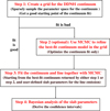 |
Fig. 1. Flowchart of our fitting tool CLIcK. |
3. CLIcK on the observed spectrum of AA Tau
AA Tau is a classical T Tauri star located in the Taurus star formation region at a distance of ∼137 pc (Gaia Collaboration 2016, 2018). The spectral type of the star is M0.6 and the stellar mass ∼0.6 M⊙ (Herczeg & Hillenbrand 2014). AA Tau has been the focus of intense multiwavelength campaigns due its periodic dimming which is ascribed to an extended non-axisymmetric feature, such as a disk warp, passing in front of a star-disk system seen close to edge-on (e.g., Bouvier et al. 2013). Recent ALMA continuum images at ∼0.2″ resolution have revealed that the outer disk is rather inclined with respect to the observer (59°), but not edge-on (Loomis et al. 2017), providing evidence for an inner versus outer disk misalignment being responsible for the most recent long-duration dimming that started in 2011 (e.g., Rodriguez et al. 2015). Before this dimming, AA Tau was observed with the Spitzer/IRS at a spectral resolution of R ∼ 600. Carr & Najita (2008) were the first to report its molecular spectrum from 10 μm out to 37 μm which is particularly rich in water emission lines. As such, AA Tau is an excellent target with which to test and showcase our continuum and line fitting kit.
3.1. Fit to the short-wavelength IRS spectrum
The short-wavelength IRS module covers from ∼10 out to 20 μm. Carr & Najita (2008, 2011) modeled the water emission spectrum of AA Tau in the wavelength range 12−16 μm using a slab of gas in LTE. They first subtracted the observed spectrum with a user-defined continuum and then performed the line fitting. Our approach differs from Carr & Najita (2008, 2011) in that we fit the continuum and line emission together.
First, we ran a grid of dust continuum SED models to identify the one that roughly matches the observed flux density versus wavelength. Then, starting from the best continuum model, together with a set of initial parameters for the H2O slab, we find the best fit (with the minimum χ2) to the continuum and the water lines by calculating eight MCMCs, each of which contains 2000 models. The parameters determining both the continuum and the water lines are allowed to vary during the optimization. Since we are more interested in interpreting the line emission, data points at wavelengths dominated by emission lines from other species (e.g., HCN, C2H2, CO2, and OH) or by continuum alone do not contribute to the resulting χ2. Our best-fit model to the 12 − 16 μm spectrum of AA Tau is shown in black in the upper panel of Fig. 2. The lower panel of Fig. 2 presents the difference between the best fit model and the observed spectrum, with the gray shaded regions indicating the wavelengths that contribute to the χ2 calculation. We note how the model reproduces the observation well, with relative differences typically less than 5% for the full range of fitted wavelengths.
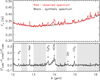 |
Fig. 2. Comparison between the observed (red) and best-fit synthetic (black) spectra in the wavelength range 12 − 16 μm. The relative difference between model and observation (Fν, obs − Fν, mod)/Fν, obs is shown in the bottom panel. The gray shaded regions indicate the data points that contribute to the χ2 calculation in fitting the water spectrum. Prominent emission lines from other molecules are shown. |
To determine the confidence intervals of the best-fit parameters, we ran a dense grid of models with the gas temperature varying between Tbest − 150 K and Tbest + 150 K (in steps of 5 K), column density between Log(Nbest)−1.5 and Log(Nbest)+1.5 (in logarithmic steps of 0.05) and emitting area between Re, best − 1.5 AU and Re, best + 1.5 AU (in steps of 0.1 AU), where the subscript “best” refers to the best-fit values. Then, a Bayesian analysis was performed to calculate the probability distribution for each parameter (Fig. 3), from which we computed 68% of the area under the functions to assign 1σ uncertainties. We placed strong constraints on the water column density and temperature, as illustrated by the clear peaks in the corresponding probability distributions and by the minor discrepancies between these peaks and the best-fit values (see Fig. 3). Within 2σ, our best-fit parameters are the same as those reported in Carr & Najita (2008, 2011) (see Table 1), demonstrating the applicability of our fitting kit.
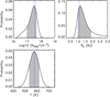 |
Fig. 3. Bayesian probability distributions of the H2O parameters for AA Tau. These distributions are used to evaluate the 68% confidence intervals (shaded regions) of the best-fit model presented in Fig. 2. The blue vertical dashed lines give the best-fit values. |
Modeling results obtained when fitting the 12 − 16 μm H2O lines in the AA Tau IRS spectrum.
3.2. Fit to the long-wavelength IRS spectrum
Using the same optimization process described above, we fit the water lines shown in the IRS spectrum from 19 to 32 μm. The best-fit synthetic spectrum is in good agreement with the observed one (see Fig. 4). We find that the best-fit temperature ( K, Table 2) is lower than the value obtained from fitting the spectrum at shorter wavelengths (
 K; see Table 1), while the emitting radius is slightly larger, though the same within the uncertainty. This is as expected because emission lines at shorter wavelengths predominately trace a hotter disk region that is closer to the central star.
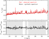 |
Fig. 4. Same as in Fig. 2, but for a fit to the water lines in the wavelength range from 19 to 32 μm. |
Modeling results obtained when fitting the 19 − 32 μm H2O lines in the AA Tau IRS spectrum.
3.3. Fit to the entire IRS spectrum
Finally, we tested our tool by fitting almost the entire water spectrum, from 12 to 32 μm. This was challenging for previous methods (see Sect. 1) as it is difficult to correctly identify the global continuum in rich molecular spectra obtained at relatively poor spectral resolution. The only attempt to retrieve molecular parameters for the entire IRS spectrum was made by Salyk et al. (2011). Instead of identifying the global continuum and fitting the entire spectrum, Salyk et al. (2011) identified 65 relatively isolated water lines, subtracted local continua, and fitted their peak emission assuming a slab of gas in LTE with one temperature. Here we use our tool to fit the continuum and the water lines adopting two temperature profiles: a constant temperature (isothermal slab) and a radially decreasing power-law profile.
The upper panel of Fig. 5 shows a comparison between the best-fit synthetic spectrum for the isothermal slab and the observation, while Table 3 reports the best-fit parameters. Our tool does a good job in reproducing the continuum and line emission as the relative difference between the synthetic and observed spectrum is smaller than 5% for most of the considered wavelengths. The isothermal slab best-fit temperature ( K) and emitting area (
 AU) are between those obtained by fitting only the short-wavelength portion (see Table 1) and only the long-wavelength portion (see Table 2) of the spectrum. This is as expected, and further demonstrates that our tool is working properly. We also note that our best-fit temperature is higher and emitting region is larger than those reported by Salyk et al. (2011), while the water column density is lower (see Table 3). Salyk et al. (2011) commented that fitting continuum-subtracted spectra instead of individual line peaks results in higher temperatures, which agrees with our finding, but also in higher column density and a smaller emitting area, which is the opposite of what we find. However, as the latter two quantities are degenerate5, increasing column density coupled with a decrease in emitting area, or vice versa, will produce model fits of similar quality.
The bottom panel of Fig. 5 show the fitting results for a radially decreasing power-law temperature profile. Observations with a broad wavelength coverage are sensitive to a range of gas temperatures. Consequently, this model provides an even better fit to the data than the isothermal slab, as shown by the lower χ2 (see Table 3). Even if we take into account the fact that this new model has one more free parameter, the conclusion holds because the number of fitted data points is much larger than the dimensionality of the model. Figure 6 presents the gas and dust temperature of the best-fit model, both of which share a similar power-law exponent. Moreover, the gas is hotter than the dust in the surface layer, which is consistent with circumstellar disk models that properly treat heating and cooling (e.g., Najita et al. 2011; Akimkin et al. 2013; Du & Bergin 2014).
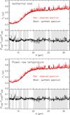 |
Fig. 5. Same as in Fig. 2, but the IRS spectrum of a broad wavelength range from 12 to 32 μm is considered in the fitting procedure. The temperature in the slab is assumed to be constant (upper panel) and to follow a radially decreasing power-law profile T = T1 AU × Rp (bottom panel). |
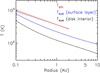 |
Fig. 6. Temperature distribution for the gas (red), dust in the surface layer (blue), and disk interior (black) of the model presented in the bottom panel of Fig. 5. The shaded region associated with the gas temperature indicates the confidence interval (see Table 3). |
Modeling results obtained when fitting almost the entire IRS water spectrum (12 − 32 μm) of AA Tau.
4. CLIcK on a reference model
We further test our kit by generating and then fitting a model spectrum for a circumstellar disk located in the Taurus star-forming region. The properties of the reference model are characterized by a set of parameters, which we set as priors in the simulation. We then discuss how well our tool reproduces the spectrum and retrieves the properties of the water emitting region.
The reference model consists of a star surrounded by a disk populated with dust and gas. Details about the dust density structure, dust properties, and stellar parameters are given in Sect. A.1. We first conduct continuum radiative transfer to self-consistently calculate the temperature structure of the dust using the RADMC package (Dullemond & Dominik 2004a). Previous observations and modeling suggest that dust and gas are thermally decoupled, particularly in the disk surface layers (Kamp & Dullemond 2004; Akimkin et al. 2013; Blevins et al. 2016). Therefore, we scale the gas temperature relative to the dust temperature using the results from the thermo-chemical model of Najita et al. (2011) (see Sect. A.2 for details). The resulting gas temperature, together with an abundance distribution of relevant molecular species, form the input for the line radiative transfer that is performed with the RADLite code (Pontoppidan et al. 2009). Following previous tests, we only consider water lines in the simulation (see Sect. A.2 for further details on the water abundance distribution and line radiative transfer). Finally, the output spectrum from RADLite is convolved with a spectral resolution of 2000, the same offered by the Mid-Infrared Instrument (MIRI) on board JWST.
Using the same procedure described in Sect. 3, we fit the water lines of the reference model, with the results presented in Figs. 7 and 8 and the best-fit parameters summarized in Table 4. The black line in the upper panel of Fig. 7 shows the best-fit synthetic spectrum, which indeed reproduces most of the water lines with relative differences of less than 5%. Figure 9 shows the gas temperature and water vapor column density of the reference model. In that figure we also draw the surface for dust optical depth at 20 μm equal to one (τ20 μm = 1). The shaded area encloses the contours of Log NH2O = 17, T = 160, 500 K and τ20 μm = 1. Therefore, these regions are expected to contribute to most of the water vapor emission at mid-IR wavelengths. Our best-fit column density (NH2O = 7.2 × 1017 cm−2), emitting area (Re = 5 AU), and temperature (T = 370 K, P = −0.28) closely match the water vapor properties in the disk regions where most of the emission comes out (see Fig. 9). This agreement shows that our tool is capable of correctly retrieving the properties of the emitting gas, even though it cannot constrain the vertical distribution of the molecules. The water vapor mass in the emitting region is ∼40% of the total water vapor mass in the reference model, in agreement with the fact that IR observations only probe a portion of the disk, e.g., the disk surface layers.
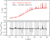 |
Fig. 7. Comparison between the reference spectrum (red) and the best-fit synthetic spectrum (black) obtained with CLIcK. |
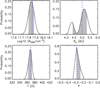 |
Fig. 8. Bayesian probability distributions of the H2O parameters for the fit to the reference spectrum. The abscissa scale in the NH2O and T panels is different here from that in Fig. 3. For the Bayesian analysis, we varied T in steps of 2.5 K, NH2O in logarithmic steps of 0.025, Re in steps of 0.1 AU, and P in steps of 0.05. The step widths for T and NH2O are smaller than those used in Fig. 3 (see Sect. 3.1). These plots show that the strong peaks are not due to an insufficient sampling of the parameters. |
Retrieved water line parameters for the reference model.
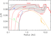 |
Fig. 9. Gas temperature and H2O column density distribution for the reference model. Contours of the gas temperature at 160, 200, 300, and 500 K are shown as red solid lines. The dashed contours refer to the water column density Log (NH2O/cm−2) at 17 (black), 18 (blue), and 19 (green), where NH2O is measured from the surface layer down to the midplane. The orange contour indicates the scale height with dust optical depth τ20 μm = 1 measured from the surface layer to the midplane. The shaded area encloses the contours of Log (NH2O/cm−2) = 17, T = 160, 500 K, and τ20 μm = 1. This region contributes to most of the water vapor emission at mid-IR wavelengths. |
5. Summary and outlook
We have developed a flexible tool called CLIcK to simultaneously fit the continuum and the line emission from circumstellar disks. The DDN01 continuum model and a slab model of gas in LTE are used to simulate the continuum and line emission, respectively; both of them are fast enough to enable large parameter studies. We applied CLIcK to fit the observed water spectrum from the AA Tau disk and found water vapor properties that are consistent with literature values obtained by fitting continuum-subtracted spectra with a slab of gas in LTE. However, CLIcK has two advantages over the past approaches: it does not require pre-defining a global or local continuum and, in the fitting procedure, it accounts for any pseudo-continuum arising from hot molecular emission lines. We have also demonstrated that CLIcK can reproduce well the entire Spitzer/IRS water emission spectrum from AA Tau, especially with the power-law temperature profile option, and correctly retrieve the parameters of the water emitting region from a reference spectrum simulated with RADLite. The framework of CLIcK can be easily generalized to solve similar problems in which the dust continuum has to be properly treated, including fitting the emission features from crystalline silicates (e.g., Juhász et al. 2010) and polycyclic aromatic hydrocarbons (e.g., Seok & Li 2017) in circumstellar disks.
Given the different spectral analysis used in the literature, re-fitting Spitzer/IRS archival spectra of circumstellar disks with CLIcK will be very valuable to quantify the water content in a homogeneous way. JWST will bring a remarkable leap forward in infrared spectroscopy. The spectrometers on board JWST, e.g., MIRI (Rieke et al. 2015) with a spectral resolution of R ∼ 2000, will not only separate many blended lines but will also boost line-to-continuum ratios, resulting in a better detection of individual lines. CLIck will be a useful tool to efficiently fit the water spectrum, subtract it, and then search for additional molecules that might be present in the atmosphere of inner disks. This will help build the chemical inventory of the terrestrial planet forming region around young stars. Moreover, with an increase in sensitivity of two orders of magnitude, JWST will be able to significantly increase the sample of faint disks around low-mass stars and brown dwarfs that could be observed with Spitzer. A homogeneous analysis of these spectra with CLIcK will clarify any dependencies between gas properties and stellar mass down to the brown dwarf regime.
Molecules and atoms with low sublimation temperatures (< a few 100 K), including water.
The only exception is the CO2 detection toward HD 101412.
The fast line raytracer (FLiTs) is developed by M. Min.
This approach is advantageous in high-dimensional modeling such as those explored here.
These two parameters can be considered as scaling factors for the line strength as long as the emission lines are optically thin.
Acknowledgments
We thank the anonymous referee for the very constructive comments that improved the manuscript. YL acknowledges support from the Natural Science Foundation of China (Grant No. 11503087) and from the Natural Science Foundation of Jiangsu Province of China (Grant No. BK20181513). We thank John S. Carr for providing the reduced Spitzer/IRS spectrum of AA Tau and Klaus Pontoppidan for help with the RADLite code. We acknowledge Ewine F. van Dishoeck for insightful discussions. This material is based upon work supported by the National Aeronautics and Space Administration under Agreement No. NNX15AD94G for the program “Earths in Other Solar Systems”. The results reported herein benefited from collaborations and/or information exchange within NASA’s Nexus for Exoplanet System Science (NExSS) research coordination network sponsored by NASA’s Science Mission Directorate.
References
- Akimkin, V., Zhukovska, S., Wiebe, D., et al. 2013, ApJ, 766, 8 [NASA ADS] [CrossRef] [Google Scholar]
- Andrews, S. M., Wilner, D. J., Espaillat, C., et al. 2011, ApJ, 732, 42 [NASA ADS] [CrossRef] [Google Scholar]
- Banzatti, A., Meyer, M. R., Bruderer, S., et al. 2012, ApJ, 745, 90 [NASA ADS] [CrossRef] [Google Scholar]
- Banzatti, A., Pontoppidan, K. M., Salyk, C., et al. 2017, ApJ, 834, 152 [NASA ADS] [CrossRef] [Google Scholar]
- Blevins, S. M., Pontoppidan, K. M., Banzatti, A., et al. 2016, ApJ, 818, 22 [NASA ADS] [CrossRef] [Google Scholar]
- Bosman, A. D., Bruderer, S., & van Dishoeck, E. F. 2017, A&A, 601, A36 [NASA ADS] [CrossRef] [EDP Sciences] [Google Scholar]
- Bouvier, J., Grankin, K., Ellerbroek, L. E., Bouy, H., & Barrado, D. 2013, A&A, 557, A77 [NASA ADS] [CrossRef] [EDP Sciences] [Google Scholar]
- Brandl, B. R., Feldt, M., Glasse, A., et al. 2014, in Ground-based and Airborne Instrumentation for Astronomy V, Proc. SPIE, 9147, 914721 [Google Scholar]
- Bruderer, S., Harsono, D., & van Dishoeck, E. F. 2015, A&A, 575, A94 [NASA ADS] [CrossRef] [EDP Sciences] [Google Scholar]
- Carr, J. S., & Najita, J. R. 2008, Science, 319, 1504 [NASA ADS] [CrossRef] [PubMed] [Google Scholar]
- Carr, J. S., & Najita, J. R. 2011, ApJ, 733, 102 [NASA ADS] [CrossRef] [Google Scholar]
- Chiang, E. I., & Goldreich, P. 1997, ApJ, 490, 368 [NASA ADS] [CrossRef] [Google Scholar]
- D’Alessio, P., Calvet, N., Hartmann, L., Franco-Hernández, R., & Servín, H. 2006, ApJ, 638, 314 [NASA ADS] [CrossRef] [Google Scholar]
- Dorschner, J., Begemann, B., Henning, T., Jaeger, C., & Mutschke, H. 1995, A&A, 300, 503 [Google Scholar]
- Du, F., & Bergin, E. A. 2014, ApJ, 792, 2 [NASA ADS] [CrossRef] [Google Scholar]
- Dullemond, C. P., & Dominik, C. 2004a, A&A, 417, 159 [NASA ADS] [CrossRef] [EDP Sciences] [Google Scholar]
- Dullemond, C. P., & Dominik, C. 2004b, A&A, 421, 1075 [NASA ADS] [CrossRef] [EDP Sciences] [Google Scholar]
- Dullemond, C. P., Dominik, C., & Natta, A. 2001, ApJ, 560, 957 [NASA ADS] [CrossRef] [Google Scholar]
- Ercolano, B., & Pascucci, I. 2017, Roy. Soc. Open Sci., 4, 170114 [NASA ADS] [CrossRef] [Google Scholar]
- Fang, M., Sicilia-Aguilar, A., Wilner, D., et al. 2017, A&A, 603, A132 [NASA ADS] [CrossRef] [EDP Sciences] [Google Scholar]
- Fedele, D., Tazzari, M., Booth, R., et al. 2018, A&A, 610, A24 [NASA ADS] [CrossRef] [EDP Sciences] [Google Scholar]
- Gaia Collaboration (Prusti, T., et al.) 2016, A&A, 595, A1 [NASA ADS] [CrossRef] [EDP Sciences] [Google Scholar]
- Gaia Collaboration (Brown, A. G. A., et al.) 2018, A&A, 616, A1 [NASA ADS] [CrossRef] [EDP Sciences] [Google Scholar]
- Gordon, I. E., Rothman, L. S., Hill, C., et al. 2017, J. Quant. Spectr. Rad. Transf., 203, 3 [Google Scholar]
- Gorti, U., Hollenbach, D., Najita, J., & Pascucci, I. 2011, ApJ, 735, 90 [NASA ADS] [CrossRef] [Google Scholar]
- Gullbring, E., Hartmann, L., Briceño, C., & Calvet, N. 1998, ApJ, 492, 323 [NASA ADS] [CrossRef] [Google Scholar]
- Herczeg, G. J., & Hillenbrand, L. A. 2014, ApJ, 786, 97 [NASA ADS] [CrossRef] [Google Scholar]
- Houck, J. R., Roellig, T. L., Van Cleve, J., et al. 2004, in Optical, Infrared, and Millimeter Space Telescopes, ed. J. C. Mather, Proc. SPIE, 5487, 62 [Google Scholar]
- Jäger, C., Mutschke, H., & Henning, T. 1998, A&A, 332, 291 [NASA ADS] [Google Scholar]
- Juhász, A., Bouwman, J., Henning, T., et al. 2010, ApJ, 721, 431 [NASA ADS] [CrossRef] [Google Scholar]
- Kamp, I., & Dullemond, C. P. 2004, ApJ, 615, 991 [NASA ADS] [CrossRef] [Google Scholar]
- Kamp, I., Thi, W.-F., Meeus, G., et al. 2013, A&A, 559, A24 [NASA ADS] [CrossRef] [EDP Sciences] [Google Scholar]
- Lahuis, F., van Dishoeck, E. F., Blake, G. A., et al. 2007, ApJ, 665, 492 [NASA ADS] [CrossRef] [Google Scholar]
- Lissauer, J. J., & Stevenson, D. J. 2007, Protostars and Planets V, 591 [Google Scholar]
- Liu, Y., Madlener, D., Wolf, S., Wang, H., & Ruge, J. P. 2012, A&A, 546, A7 [NASA ADS] [CrossRef] [EDP Sciences] [Google Scholar]
- Liu, Y., Madlener, D., Wolf, S., & Wang, H.-C. 2013, Res. Astron. Astrophys., 13, 420 [NASA ADS] [CrossRef] [Google Scholar]
- Loomis, R. A., Öberg, K. I., Andrews, S. M., & MacGregor, M. A. 2017, ApJ, 840, 23 [NASA ADS] [CrossRef] [Google Scholar]
- Mandell, A. M., Bast, J., van Dishoeck, E. F., et al. 2012, ApJ, 747, 92 [NASA ADS] [CrossRef] [Google Scholar]
- Meijerink, R., Pontoppidan, K. M., Blake, G. A., Poelman, D. R., & Dullemond, C. P. 2009, ApJ, 704, 1471 [NASA ADS] [CrossRef] [Google Scholar]
- Najita, J. R., Ádámkovics, M., & Glassgold, A. E. 2011, ApJ, 743, 147 [NASA ADS] [CrossRef] [Google Scholar]
- Pascucci, I., Hollenbach, D., Najita, J., et al. 2007, ApJ, 663, 383 [NASA ADS] [CrossRef] [Google Scholar]
- Pascucci, I., Apai, D., Luhman, K., et al. 2009, ApJ, 696, 143 [NASA ADS] [CrossRef] [Google Scholar]
- Pascucci, I., Sterzik, M., Alexander, R. D., et al. 2011, ApJ, 736, 13 [NASA ADS] [CrossRef] [Google Scholar]
- Pascucci, I., Herczeg, G., Carr, J. S., & Bruderer, S. 2013, ApJ, 779, 178 [NASA ADS] [CrossRef] [Google Scholar]
- Pontoppidan, K. M., Meijerink, R., Dullemond, C. P., & Blake, G. A. 2009, ApJ, 704, 1482 [NASA ADS] [CrossRef] [Google Scholar]
- Pontoppidan, K. M., Salyk, C., Blake, G. A., et al. 2010, ApJ, 720, 887 [NASA ADS] [CrossRef] [Google Scholar]
- Pontoppidan, K. M., Salyk, C., Bergin, E. A., et al. 2014, Protostars and Planets VI, 363 [Google Scholar]
- Rieke, G. H., Wright, G. S., Böker, T., et al. 2015, PASP, 127, 584 [NASA ADS] [CrossRef] [Google Scholar]
- Rodriguez, J. E., Pepper, J., Stassun, K. G., et al. 2015, AJ, 150, 32 [NASA ADS] [CrossRef] [Google Scholar]
- Salyk, C., Pontoppidan, K. M., Blake, G. A., Najita, J. R., & Carr, J. S. 2011, ApJ, 731, 130 [NASA ADS] [CrossRef] [Google Scholar]
- Seok, J. Y., & Li, A. 2017, ApJ, 835, 291 [NASA ADS] [CrossRef] [Google Scholar]
- Shu, F. H., Adams, F. C., & Lizano, S. 1987, ARA&A, 25, 23 [Google Scholar]
- Williams, J. P., & Cieza, L. A. 2011, ARA&A, 49, 67 [NASA ADS] [CrossRef] [Google Scholar]
- Woitke, P., Min, M., Pinte, C., et al. 2016, A&A, 586, A103 [NASA ADS] [CrossRef] [EDP Sciences] [Google Scholar]
- Woitke, P., Min, M., Thi, W.-F., et al. 2018, A&A, 618, A57 [NASA ADS] [CrossRef] [EDP Sciences] [Google Scholar]
Appendix A: Simulating the infrared spectrum of the reference model
To simulate our reference spectrum we used a continuum and a line radiative transfer code. In this appendix, we provide details about both codes.
A.1. Continuum radiative transfer
Density structure. We employ the RADMC package to solve the problem of continuum radiative transfer assuming a two-dimensional flared disk model (Dullemond & Dominik 2004a). The model includes two distinct grain populations that differ in terms of dust opacity and vertical extension in the disk, i.e., a small-grain population and a large-grain population. The disk extends from an inner radius of 0.1 au to an outer radius of 200 au. The total dust mass in the disk is defined as Mdust, tot.
Small dust grains occupy a minor fraction of the dust mass, (1 − f) Mdust.tot, and are distributed vertically following a power-law profile:
 (A.1)
(A.1)
The degree of disk flaring is quantified with β, and hc represents the scale height at a fixed characteristic radius of Rc = 100 au. Conversely, most of the dust mass is composed of large dust grains, f Mdust.tot, which are concentrated close to the midplane with a scale height Λ h. The parameter Λ < 1, describing the degree of dust settling, is assumed to be constant over radius R. This is a simple approach to account for the effect of dust sedimentation in protoplanetary disks (e.g., Dullemond & Dominik 2004b; D’Alessio et al. 2006).
We model the surface density profile as a power law with an exponential taper
![Mathematical equation: $$ \begin{aligned} \Sigma \propto \left(\frac{R}{R_{c}}\right)^{-\gamma }\mathrm{exp}\left[-\left(\frac{R}{R_{c}}\right)^{2-\gamma }\right], \end{aligned} $$](/articles/aa/full_html/2019/03/aa34418-18/aa34418-18-eq23.gif) (A.2)
(A.2)
where γ is the gradient parameter.
The two-dimensional density structure for each grain population can be parameterized as
![Mathematical equation: $$ \begin{aligned} \rho _{\rm {small}}\propto \frac{(1-f)\Sigma }{h}\,\exp \left[-\frac{1}{2}\left(\frac{z}{h}\right)^2\right], \\ \end{aligned} $$](/articles/aa/full_html/2019/03/aa34418-18/aa34418-18-eq24.gif) (A.3)
(A.3)
![Mathematical equation: $$ \begin{aligned} \rho _{\rm {large}}\propto \frac{f\Sigma }{\Lambda h}\,\exp \left[-\frac{1}{2}\left(\frac{z}{\Lambda h}\right)^2\right], \\ \end{aligned} $$](/articles/aa/full_html/2019/03/aa34418-18/aa34418-18-eq25.gif) (A.4)
(A.4)
where ρsmall is the density for the small-grain population and ρlarge is the density for the large-grain population. Our parameterization of the density structure has been used to successfully model multiwavelength observations of protoplanetary disks in the literature (e.g., Andrews et al. 2011; Fang et al. 2017; Fedele et al. 2018). Table A.1 summarizes the input parameters and the values we chose for the reference model.
Dust properties. The dust in the model is a mixture of 75% amorphous silicate and 25% carbon, with complex refractive indices given by Dorschner et al. (1995) and Jäger et al. (1998). Mie theory is used to calculate the dust opacities. The grain size distribution follows the standard power law dn(a)∝a−3.5da with a minimum grain size of amin = 0.01 μm. The maximum grain size is set to amax = 1 μm for the small grain population and amax = 1 mm for the large grain population.
Parameters of the reference model.
Stellar heating. We assume that the disk is passively heated by stellar irradiation. The stellar parameters are adopted as the average properties of a T Tauri star described by Gullbring et al. (1998). The stellar temperature and luminosity are T⋆ = 4000 K and L⋆ = 0.92 L⊙, respectively. The stellar spectrum is modeled as a blackbody.
A.2. Line radiative transfer
As we intend to retrieve the properties of water vapor, we only simulate a mid-IR spectrum for the water lines. The line radiative transfer is performed with the RADLite code (Pontoppidan et al. 2009), which is a line raytracer designed to quickly render spectra and images of complex line emission from protoplanetary disks. The molecular parameters for water are taken from the 2016 edition of the HITRAN database (Gordon et al. 2017). The level populations are assumed in local thermodynamic equilibrium, set by the local gas temperature. The local line broadening is set to 0.9 cs, where cs is the sound speed.
Gas temperature. We obtained the disk dust temperature by solving the problem of continuum radiative transfer in Sect. A.1. However, we cannot assume that the gas temperature is the same as the dust temperature throughout the disk as models that properly account for heating and cooling have shown that this assumption breaks down especially in the disk upper layers where the gas is directly exposed to ultraviolet and X-ray irradiation from the central star and from the interstellar radiation field (e.g., Kamp & Dullemond 2004; Akimkin et al. 2013; Du & Bergin 2014). Following the approach introduced by Blevins et al. (2016), specifically their Case II, we scaled the gas temperature relative to the dust temperature. This approach is based on the thermo-chemical model presented in Najita et al. (2011), in particular their Fig. 1 which provides the scaling factor as a function of disk radius and hydrogen column density. The blue contours in our Fig. 9 show the resulting gas temperature of the reference model.
Water vapor abundance. For simplicity, we assumed a constant abundance for water vapor in the disk:  , where g2d = 100 is the gas-to-dust mass ratio and Xc = 10−4 is the canonical abundance for water. The abundance is set to zero at low hydrogen column densities, NH ≲ 1021 cm−2, to account for efficient photo-destruction (Najita et al. 2011). At temperatures lower than ∼160 K, water is expected to condense onto dust grains. Therefore, we set the abundance at these places to a tiny value. The red dashed contours in Fig. 9 show the column density of water vapor measured from the disk upper layer to the midplane of the reference model.
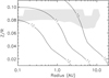 |
Fig. A.1. Gas density Log (ngas/cm−3) of the reference model at 10, 11, and 12, respectively. The shaded area is identical to that in Fig. 9. In the water emitting region, the gas density is close to or larger than the critical density, which implies that our LTE approximation is valid. |
We focused on water lines in the wavelength range of 14 − 20 μm, which is covered by the Spitzer/IRS and the upcoming JWST/MIRI instruments. The red line in Fig. 7 shows the spectrum of the reference model after convolving with a spectral resolution of 2000, similar to that offered by JWST/MIRI.
LTE approximation. In RADLite, we assumed LTE excitation to simulate the reference spectrum, which makes the subsequent parameter retrieval fair because CLIcK calculates line emission based on the LTE assumption as well. Mid-IR water lines are dominated by pure rotational transitions. The critical densities for exciting these lines (at the wavelengths considered here, 14 ≤ λ ≤ 20 μm) are in the range of 108 − 1011 cm−3. In disk regions that contribute most of the water line fluxes, the gas density is comparable with the critical densities (see Fig. A.1), and the gas is warmer than the dust because the gas temperature is set by scaling the dust temperature based on the thermo-chemical model given in Najita et al. (2011). Therefore, LTE assumption is relatively reasonable in our case. It is beyond the scope of this paper to discuss whether the gas is really in LTE. Nevertheless, detailed non-LTE excitation calculations have shown that there is no dramatic deviation of the water line fluxes (e.g., Meijerink et al. 2009; Woitke et al. 2018). Similar conclusions also hold for the mid-IR HCN and CO2 lines (Bruderer et al. 2015; Bosman et al. 2017). The abundances derived by LTE and non-LTE models do not differ by a large factor. Non-LTE excitation probably has a noticeable impact on the line shape as the emitting region can be much larger than in LTE models. However, observations with a high spectral resolving power (e.g., R ∼ 5000 offered by E-ELT/METIS, Brandl et al. 2014) are required to distinguish the two scenarios.
All Tables
Modeling results obtained when fitting the 12 − 16 μm H2O lines in the AA Tau IRS spectrum.
Modeling results obtained when fitting the 19 − 32 μm H2O lines in the AA Tau IRS spectrum.
Modeling results obtained when fitting almost the entire IRS water spectrum (12 − 32 μm) of AA Tau.
All Figures
|
Fig. 1. Flowchart of our fitting tool CLIcK. |
| In the text | |
|
Fig. 2. Comparison between the observed (red) and best-fit synthetic (black) spectra in the wavelength range 12 − 16 μm. The relative difference between model and observation (Fν, obs − Fν, mod)/Fν, obs is shown in the bottom panel. The gray shaded regions indicate the data points that contribute to the χ2 calculation in fitting the water spectrum. Prominent emission lines from other molecules are shown. |
| In the text | |
|
Fig. 3. Bayesian probability distributions of the H2O parameters for AA Tau. These distributions are used to evaluate the 68% confidence intervals (shaded regions) of the best-fit model presented in Fig. 2. The blue vertical dashed lines give the best-fit values. |
| In the text | |
|
Fig. 4. Same as in Fig. 2, but for a fit to the water lines in the wavelength range from 19 to 32 μm. |
| In the text | |
|
Fig. 5. Same as in Fig. 2, but the IRS spectrum of a broad wavelength range from 12 to 32 μm is considered in the fitting procedure. The temperature in the slab is assumed to be constant (upper panel) and to follow a radially decreasing power-law profile T = T1 AU × Rp (bottom panel). |
| In the text | |
|
Fig. 6. Temperature distribution for the gas (red), dust in the surface layer (blue), and disk interior (black) of the model presented in the bottom panel of Fig. 5. The shaded region associated with the gas temperature indicates the confidence interval (see Table 3). |
| In the text | |
|
Fig. 7. Comparison between the reference spectrum (red) and the best-fit synthetic spectrum (black) obtained with CLIcK. |
| In the text | |
|
Fig. 8. Bayesian probability distributions of the H2O parameters for the fit to the reference spectrum. The abscissa scale in the NH2O and T panels is different here from that in Fig. 3. For the Bayesian analysis, we varied T in steps of 2.5 K, NH2O in logarithmic steps of 0.025, Re in steps of 0.1 AU, and P in steps of 0.05. The step widths for T and NH2O are smaller than those used in Fig. 3 (see Sect. 3.1). These plots show that the strong peaks are not due to an insufficient sampling of the parameters. |
| In the text | |
|
Fig. 9. Gas temperature and H2O column density distribution for the reference model. Contours of the gas temperature at 160, 200, 300, and 500 K are shown as red solid lines. The dashed contours refer to the water column density Log (NH2O/cm−2) at 17 (black), 18 (blue), and 19 (green), where NH2O is measured from the surface layer down to the midplane. The orange contour indicates the scale height with dust optical depth τ20 μm = 1 measured from the surface layer to the midplane. The shaded area encloses the contours of Log (NH2O/cm−2) = 17, T = 160, 500 K, and τ20 μm = 1. This region contributes to most of the water vapor emission at mid-IR wavelengths. |
| In the text | |
|
Fig. A.1. Gas density Log (ngas/cm−3) of the reference model at 10, 11, and 12, respectively. The shaded area is identical to that in Fig. 9. In the water emitting region, the gas density is close to or larger than the critical density, which implies that our LTE approximation is valid. |
| In the text | |
Current usage metrics show cumulative count of Article Views (full-text article views including HTML views, PDF and ePub downloads, according to the available data) and Abstracts Views on Vision4Press platform.
Data correspond to usage on the plateform after 2015. The current usage metrics is available 48-96 hours after online publication and is updated daily on week days.
Initial download of the metrics may take a while.