| Issue |
A&A
Volume 623, March 2019
|
|
|---|---|---|
| Article Number | A44 | |
| Number of page(s) | 17 | |
| Section | Stellar atmospheres | |
| DOI | https://doi.org/10.1051/0004-6361/201834114 | |
| Published online | 05 March 2019 | |
The CARMENES search for exoplanets around M dwarfs
Activity indicators at visible and near-infrared wavelengths★
1
Institut für Astrophysik,
Friedrich-Hund-Platz 1,
37077 Göttingen,
Germany
e-mail: schoefer@astro.physik.uni-goettingen.de
2
Max-Planck-Institut für Sonnensystemforschung,
Justus-von-Liebig-Weg 3,
37077 Göttingen, Germany
3
Hamburger Sternwarte,
Gojenbergsweg 112,
21029 Hamburg, Germany
4
Institut de Ciències de l’Espai (ICE, CSIC), Campus UAB, c/ de Can Magrans s/n,
08193 Bellaterra,
Barcelona, Spain
5
Institut d’Estudis Espacials de Catalunya (IEEC),
08034
Barcelona, Spain
6
Landessternwarte, Zentrum für Astronomie der Universität Heidelberg,
Königstuhl 12,
69117 Heidelberg, Germany
7
Instituto de Astrofísica de Andalucía (IAA-CSIC),
Glorieta de la Astronomía s/n,
18008
Granada, Spain
8
Centro de Astrobiología (CSIC-INTA), ESAC Campus,
Camino Bajo del Castillo s/n,
28692 Villanueva de la Cañada,
Madrid, Spain
9
School of Physics and Astronomy, Queen Mary, University of London,
327 Mile End Road,
London E1 4NS, UK
10
Instituto de Astrofísica de Canarias,
Vía Láctea s/n,
38205 La Laguna,
Tenerife, Spain
11
Departamento de Astrofísica, Universidad de La Laguna,
38206 La Laguna,
Tenerife, Spain
12
Thüringer Landessternwarte Tautenburg,
Sternwarte 5,
07778 Tautenburg, Germany
13
Max-Planck-Institut für Astronomie,
Königstuhl 17,
69117
Heidelberg, Germany
14
Departamento de Astrofísica y Ciencias de la Atmósfera, Facultad de Ciencias Físicas, Universidad Complutense de Madrid,
28040 Madrid, Spain
15
Centro Astronómico Hispano-Alemán (CSIC-MPG), Observatorio Astronómico de Calar Alto, Sierra de los Filabres,
04550 Gérgal, Almería, Spain
16
School of Geosciences, Raymond and Beverly Sackler Faculty of Exact Sciences, Tel Aviv University,
6997801
Tel Aviv, Israel
Received:
21
August
2018
Accepted:
18
January
2019
Context. The Calar Alto high-Resolution search for M dwarfs with Exo-earths with Near-infrared and optical Echelle Spectrographs (CARMENES) survey is searching for Earth-like planets orbiting M dwarfs using the radial velocity method. Studying the stellar activity of the target stars is important to avoid false planet detections and to improve our understanding of the atmospheres of late-type stars.
Aims. In this work we present measurements of activity indicators at visible and near-infrared wavelengths for 331 M dwarfs observed with CARMENES. Our aim is to identify the activity indicators that are most sensitive and easiest to measure, and the correlations among these indicators. We also wish to characterise their variability.
Methods. Using a spectral subtraction technique, we measured pseudo-equivalent widths of the He I D3, Hα, He I λ10833 Å, and Pa β lines, the Na I D doublet, and the Ca II infrared triplet, which have a chromospheric component in active M dwarfs. In addition, we measured an index of the strength of two TiO and two VO bands, which are formed in the photosphere. We also searched for periodicities in these activity indicators for all sample stars using generalised Lomb-Scargle periodograms.
Results. We find that the most slowly rotating stars of each spectral subtype have the strongest Hα absorption. Hα is correlated most strongly with He I D3, whereas Na I D and the Ca II infrared triplet are also correlated with Hα. He I λ10833 Å and Paβ show no clear correlations with the other indicators. The TiO bands show an activity effect that does not appear in the VO bands. We find that the relative variations of Hα and He I D3 are smaller for stars with higher activity levels, while this anti-correlation is weaker for Na I D and the Ca II infrared triplet, and is absent for He I λ10833 Å and Paβ. Periodic variation with the rotation period most commonly appears in the TiO bands, Hα, and in the Ca II infrared triplet.
Key words: stars: activity / stars: late-type / stars: low-mass
The full version of Table A.1 is only available at the CDS via anonymous ftp to cdsarc.u-strasbg.fr (130.79.128.5) or via http://cdsarc.u-strasbg.fr/viz-bin/qcat?J/A+A/623/A44
© ESO 2019
1. Introduction
Because of their low masses and temperatures, M dwarfs have become interesting targets for radial velocity surveys, as Earth-like planets orbiting in their liquid-water habitable zones induce Doppler variations in the order of 1 m s−1. To reach this level of radial velocity precision, the Calar Alto high-Resolution search for M dwarfs with Exo-earths with Near-infrared and optical Échelle Spectrographs (CARMENES, Quirrenbach et al. 2018) uses two spectrograph channels simultaneously that cover the visible wavelength range from 5200 to 9600 Å and the near-infrared wavelength range from 9600 to 17 100 Å, where M dwarfs emit most of their flux.
The CARMENES sample consists of the brightest M dwarfs of each spectral subtype that are observable from Calar Alto (Reiners et al. 2018). Despite the focus on finding planets, active stars were not removed from the sample, enabling us to study the stellar activity of a statistically significant sample.
One challenge for using the radial velocity method to find exoplanets around M dwarfs is that stellar activity can cause additional variations of the same order of magnitude as the signal induced by the planet (e.g. Barnes et al. 2014). It is therefore crucial to quantify the activity of the target stars in terms of strength and variability. Indicators derived from the cross-correlation function such as bisectors (Queloz et al. 2001) are closely connected to the effects of stellar activity on radial velocity measurements, whereas high-precision photometry traces starspots (e.g. Aigrain et al. 2012). A third approach, which is directly related to the physical processes in the stellar atmosphere, is to examine spectral lines that are sensitive to activity. While the Ca II H&K lines have been established as the standard activity indicator in Sun-like stars (e.g. Wilson 1968; Baliunas et al. 1995), M dwarfs emit considerably less flux at these short wavelengths, which are therefore not covered by CARMENES. Late-type M dwarfs in particular are rarely included in Ca II H&K surveys because they are faint at short wavelengths, and the Hα line has instead been widely used to characterise the activity in samples of M dwarfs (e.g. Stauffer & Hartmann 1986; West et al. 2004; Jeffers et al. 2018). Unlike Ca II H&K, however, Hα may give ambiguous results at low activity levels because it is expected to be an increasingly deep absorption line at first with increasing activity, then fill in, and finally go into emission (Cram & Mullan 1979).
In addition to Hα, other lines in the range of the visible channel of CARMENES that have been found to have chromospheric components sensitive to activity are the He I D3 (hereafter He D3) line, the Na I D (hereafter Na D) doublet, and the Ca II infrared triplet (hereafter Ca IRT; e.g. Gizis et al. 2002; Houdebine et al. 2009; Robertson et al. 2016; Martin et al. 2017). With the near-infrared channel, the He I λ10833 Å (hereafter He 10833) and Paβ lines are accessible. They have also been investigated as chromospheric activity diagnostics in M dwarfs (e.g. Zirin 1982; Short & Doyle 1998; Sanz-Forcada & Dupree 2008; Schmidt et al. 2012). Another way to study the activity of M dwarfs is to examine titanium oxide and vanadium oxide absorption bands formed in the photosphere. Being sensitive to temperature, the strength of these bands can be affected by starspots. Moreover, the absorption bands of titanium oxide are sensitive to magnetic fields (Berdyugina & Solanki 2002), but also to metallicity (e.g. Bessell 1982; Lépine et al. 2007), which is not related to activity.
In this paper we present an overview of pseudo-equivalent width measurements of the spectral lines that are sensitive to chromospheric activity at visible-light and near-infrared wavelengths using a spectral subtraction technique, and indices of photospheric TiO and VO bands for 331 stars of the CARMENES sample. We evaluate the sensitivity of these lines and investigate correlations among these activity indicators. Additionally, we explore the variations of these indicators for each star both in terms of the total variation and in view of periodicities.
The paper is structured as follows: we describe the observations in Sect. 2. In Sect. 3 we present our measurement methods. Section 4 gives an overview of the measured activity indicators and investigates how they are correlated, and Sect. 5 explores how the activity indicators for each star vary in time. Finally, we summarise our results in Sect. 6.
2. Observations
The CARMENES spectrograph is mounted on the 3.5 m telescope at the Calar Alto Observatory. A beam splitter in the telescope front-end separates the visible from the near-infrared light at a wavelength of 9600 Å. While both spectrograph channels operate independently, the same object can therefore be observed simultaneously with both spectrographs. The visible-light spectrograph provides a spectral resolution of R = 94 600 in the wavelength range from 5200 to 9600 Å with a mean sampling of 2.8 spectral bins per resolution element, and the near-infrared spectrograph covers the wavelength range from 9600 Å to 17 100 Å with a spectral resolution ofR = 80 400 and a mean sampling of 2.5 spectral bins per resolution element (Quirrenbach et al. 2018).
The CARMENES sample is composed of the brightest stars for each spectral subtype from M0.0 to M9.0 V that are observable from Calar Alto (δ > −23°). Where available, we use the spectral types derived by Alonso-Floriano et al. (2015), Lépine et al. (2013), or Reid et al. (1995) from band indices in low-resolution spectra. For 30 stars not included in these catalogues, we use spectral types from various other sources (Kirkpatrick et al. 1991; Lépine et al. 2003; Scholz et al. 2005; Gray et al. 2003, 2006; Riaz et al. 2006; Schmidt et al. 2007; Jenkins et al. 2009; Shkolnik et al. 2009; Gigoyan et al. 2010; Newton et al. 2014; David et al. 2016; Benneke et al. 2017; Hirano et al. 2018). While Cortés-Contreras et al. (2017) and Jeffers et al. (2018) identified binaries with a separation of less than 5 arcsec during the target preselection, Baroch et al. (2018) discovered nine further double-lined spectroscopic binaries during the CARMENES survey. The separation of activity indicators in spectroscopic binaries is beyond the scope of this paper, and we therefore exclude these binaries. With this restriction, our sample consists of 331 stars, which are tabulated in Table A.1. It includes not only the 324 CARMENES survey stars presented by Reiners et al. (2018), but also 7 stars that were added to the survey later. As a consequence of selecting the brightest stars for each spectral subtype, our sample is focused on the solar neighbourhood and does not contain many stars from more distant and older populations. Of the 331 investigated stars, 98 stars were identified as members of the young disc population, 181 stars are in the thin disc, 13 stars in transition between thin and thick discs, and 23 stars in the thick disc (Montes et al. 2001; Cortés-Contreras 2016).
In this work, we analyse a total of 11 000 visible and 10 500 near-infrared spectra obtained between 3 January 2016 and 10 July 2018. The observations were not evenly distributed among the sample: while 103 stars were observed fewer than 10 times, 23 stars were observed more than 100 times. The spectra were reduced with the CARACAL pipeline using the flat-relative optimal extraction (Zechmeister et al. 2014). Additionally, a co-added spectrum of each star was computed from all individual spectra using SERVAL (Zechmeister et al. 2018). The co-added spectra provide an increased signal-to-noise ratio (S/N) and were corrected for telluric lines, which appear in different positions in the individual spectra because of different barycentric velocities at different observation times. To explore the activity indicators across the sample, we derived an average value for each star from the co-added spectrum instead of averaging the indicators measured in individual spectra. This reduces the impact of outliers like strong flaring events, as data points outlying by more than 5σ are excluded from the co-adding. The results from individual spectra were used for investigating the variations in activity indicators for each star.
3. Activity indicators
In this section we describe the activity indicators and our measurement methods. As Ca II H&K are not covered by CARMENES, we used the Hα line as our main indicator of chromospheric activity. While Gizis et al. (2002) reported a correlation between the emission strengths in Hα and He D3, Houdebine et al. (2009) noted that the He D3 line is in emission if there is emission in Na D. Therefore, we included both the He D3 line and the Na D doublet in our study. The Na D doublet also has a strong photospheric absorption component that is sensitive to effective temperature, metallicity, and pressure, and it has therefore been used as an indicator for spectral type, metallicity, and luminosity class (Luyten 1923; Spinrad 1962; Covey et al. 2007). Towards the red end of the visible-light spectra, the Ca IRT lines show chromospheric emission in active stars (Mallik 1997; Martin et al. 2017). Like the Na D doublet, the Ca IRT lines have strong photospheric absorption components that are sensitive to effective temperature, metallicity, and surface gravity (Jones et al. 1984; Jorgensen et al. 1992). We did not include the K I λ7700 Å and the Na I λ8200 Å doublets, which were investigated by Robertson et al. (2016), because they are located in spectral regions with strong telluric contamination. In the wavelength range covered by the near-infrared channel, Schmidt et al. (2012) observed the He 10833 and Paβ lines in emission during M dwarf flares. The higher order lines of the Paschen series require higher excitation energies and therefore appear weaker, whereas the Paα line is outside our spectral range.
Among the photospheric TiO absorption bands, the γ band at 7050 Å and the ϵ band at 8430 Å are very sensitive to the effective temperature (Kirkpatrick et al. 1993). Of the several photospheric VO absorption bands that have been used for spectral typing in late-M dwarfs and L dwarfs (Kirkpatrick et al. 1999; Martín et al. 1999) because of their sensitivity to cooler temperatures, we selected the bands at 7436 and 7942 Å because only few other spectral lines lie close to the band heads.
3.1. Pseudo-equivalent widths
As a measure of the chromospheric activity strength, we used the equivalent widths of the spectral lines selected above. Because M dwarf spectra do not show extensive continuum ranges, the equivalent width was defined with respect to a pseudo-continuum and is therefore called a pseudo-equivalent width (pEW).
To completely measure the emission caused by activity, we chose our integration windows λ0 ± Δλ to be sufficiently broad for the broadest emission lines seen in the analysed spectra. By using the integration windows listed in Table 1, we included most of the emission even in case of a strong flaring event. The disadvantage of broad integration windows is that they also include other nearby absorption lines. To minimise the effects of nearby lines and the photospheric absorption components of the Na D and Ca IRT lines, we used a spectral subtraction technique similar to what has been reported by Young et al. (1989) and Montes et al. (1995), and subtracted the spectrum of an inactive reference star.
We expect the strengths of photospheric absorption lines to depend mainly on the effective temperature, therefore wegroup our sample stars by spectral subtype. While metallicity and surface gravity also affect the photospheric absorption, especially in the cases of the Na D and the Ca IRT lines, we did not use a more detailed classification because this would lead to a large number of small groups that might not contain any inactive reference star, and the results for stars of different groups are not comparable without accounting for the different reference stars. Our reference star in each group was the star with the longest known rotation period Prot. We assumed that these are the least active stars of each spectral subtype because the relation between chromospheric activity and stellar rotation is well established (e.g. Delfosse et al. 1998; Mohanty & Basri 2003; Newton et al. 2017; Jeffers et al. 2018). The disadvantage of this choice is that Prot is known for only 154 of our 331 sample stars, so that our sample may include even slower rotators and hence less active stars. Our reference stars for spectral subtypes M0.5 and M2.0 have considerably shorter rotation periods than the other reference stars, so that it is likely that there are slower rotators with an undetected rotation period among the stars of these subtypes in our sample. On the other hand, this choice is independent of our measurements and does not rely on other measurements of the Hα line. This is an advantage because according to Cram & Mullan (1979), Hα behaves ambiguously at low activity levels, as it first goes into deeper absorption before it is filled in and goes into emission with increasing activity strength. For spectral subtypes M5.5 and M6.0, however, all stars in our sample with a known rotation period have Hα in emission, so that we instead selected the stars without Hα emission as the reference stars for these subtypes. For stars of spectral subtype later than M6.0, we used the same reference star as for spectral type M6.0 because there are no very late-type stars without Hα emission in our sample. All reference stars are listed in Table 2. As shown in Fig. 1, all reference stars have Hα in absorption, which indicates a minimum level of chromospheric heating that is necessary to excite hydrogen atoms. However, the reference stars do not show emission in the line wings, which we observe in stars with significantly less Hα absorption. We therefore conclude that our reference stars are among the least active stars in our sample, although they have a minimum level of chromospheric activity.
The subtraction of the co-added spectrum of the reference star from the investigated spectrum requires several preparation steps. First, we applied rotational broadening to the co-added spectrum of the reference star if the investigated star shows measurable rotational velocity values (v sin i) above the detection limit of 2 km s−1 (Reiners et al. 2018). Next, we transformed both spectra to a common wavelength grid by correcting for the Doppler shift between them. To determine the Doppler shift, we calculated the cross-correlation function of the spectral order that contains the considered spectral line and fit a Gaussian to the highest peak. After this, we normalised both spectra to their mean flux in the left and right pseudo-continuum ranges λl∕r ± ΔλPC located on either side of the considered line, which are given in Table 1 and shown in Fig. 2. We then have the normalised, shifted spectrum S(λ) and the normalised, broadened reference star spectrum T(λ).
We define the pseudo-continuum PC(λ) as a linear interpolation between the pseudo-continuum ranges of T(λ):
 (1)
(1)
where PCl∕r is defined as the 90th percentile of T(λ) in the pseudo-continuum ranges λl∕r ± ΔλPC, which is robust to both the noise level and stellar absorption lines in the reference star spectrum.
For reasons of clarity, we denote the pseudo-equivalent width measured after the spectral subtraction as pEW′ and then calculated it as
 (2)
(2)
We approximated the integral using the trapezoidal rule. To be consistent with the traditional definition of the equivalent width, positive values indicate absorption in the residual spectrum, while negative values indicate emission. We identified the inverse root mean square (rms) of the residual spectrum in the pseudo-continuum ranges as the S/N and estimated the uncertainty of the pseudo-equivalent width using the formula derived by Vollmann & Eversberg (2006), which with our conventions and ⟨R⟩ the mean of the residual spectrum within the line window λ0 ± Δλ becomes
 (3)
(3)
We note that pEW′ refers to thepseudo-equivalent width measured after the spectral subtraction as opposed to pEW without spectral subtraction.
Despite the narrow integration windows for the He 10833 and Paβ lines, telluric contamination depending on the Doppler shift of the stellar spectrum still remained. Therefore, we discarded  measurements where the observed absolute radial velocity including the barycentric motion of Earth was between 14 and 125 km s−1, and
  measurements where it wasbetween 10 and 43 km s−1.
Integration windows and pseudo-continuum ranges for pEW’ measurements of the selected lines that are sensitive to chromospheric activity.
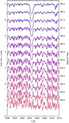 |
Fig. 1. Hα region in the co-added spectra of the slow-rotating, Hα inactive reference stars given in Table 2. |
Reference stars for each spectral subtype.
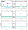 |
Fig. 2. Selected spectra in regions around the considered chromospheric lines: an inactive M0.0 star (J14257+236W, black), a moderately active M2.0 star (J18174+483, purple), a very active M3.5 star (J22468+443) in flaring (green) and quiescent state (blue), and a moderately active M7.0 star (J02530+168, orange). The region around the He D3 and Na D lines (top left panel) in the M7.0 spectrum is not shown because of a low signal-to-noise ratio. Bars mark the line windowranges (solid) and pseudo-continuum ranges (dashed) as given in Table 1. In the case of Hα, we also show the line window and pseudo-continuum ranges used by Jeffers et al. (2018; red) and by Reid et al. (1995) and Alonso-Floriano et al. (2015; blue). |
3.2. Photospheric band indices
In case of the photospheric TiO and VO absorption bands, the pseudo-equivalent width is not a good measure to quantify the strength because they may extend over multiple spectral orders and are blended with other spectral features. Instead, we measured indices derived from the mean fluxes in two small ranges on either side of the band head:
 (4)
(4)
with the numerator and denominator ranges given in Table 3 and shown in Fig. 3. Similar indices have been used previously to measure the strength of photospheric absorption bands (e.g. Reid et al. 1995; Kirkpatrick et al. 1999). However, they were derived for low-resolution spectra using greater numerator and denominator ranges. Because these ranges also include other spectral features, the resulting indices are a less accurate measure of the absorption band strength.
Following Zechmeister et al. (2018), we estimated the error of the mean fluxes from the data error ϵi of each bin in the considered spectral range as
 (5)
(5)
and calculated the uncertainty of the index by propagating these errors:
 (6)
(6)
Using these formulations, we calculated the activity indicators for individual observations and the co-added spectra for all 331 stars in our sample.
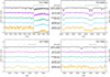 |
Fig. 3. Same spectra as in Fig. 2 in regions around the considered photospheric bands. Bars mark the numerator ranges (solid) and denominator ranges (dashed) as given in Table 3. |
Numerator and denominator ranges for photospheric absorption band indices.
4. Analysis of results from co-added spectra
This section analyses the activity indicators derived from the co-added spectra that are listed in Table A.1. We show the spectral type dependence of the activity indicators and compare our results to those of previous M dwarf activity studies. In addition, we investigate the correlations among the chromospheric indicators and the effects of activity on the photospheric bands.
4.1. Spectral-type dependence of activity indicators
As an overview of our measured quantities, we show the spectral type dependence of the pEW′ and indices derived from the co-added spectra for each of the 331 sample stars. This serves to demonstrate the effect of the spectral subtraction technique in the pEW′ calculation and to motivate the investigation of correlations among the different indicators.
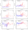 |
Fig. 4. pEW′ of chromospheric lines as a function of spectral type. |

4.1.1. Chromospheric lines
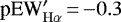
We plot the pEW′ of the chromospheric lines as a function of spectral type in Fig. 4. We note that by definition, the reference stars used for the spectral subtraction technique have pEW′ = 0 Å for all lines. Stars with  Å are marked as Hα active. This threshold is considerably different from previous M dwarf activity studies, which defined activity thresholds of −0.5 (Jeffers et al. 2018), −0.75 (West et al. 2011), or −1 Å (Newton et al. 2017), for instance, for pEWHα without spectral subtraction, that is, emission with respect to the pseudo-continuum rather than excess emission with respect to a reference star with Hα absorption. However, we find that relatively few stars have
  Å, and therefore small variations or a slightly different activity threshold do not significantly change the number of Hα active stars. The threshold of
  Å is further justified in Sect. 5.1.
For He D3, we find that all Hα inactive stars have values comparable to the reference star of their spectral subtype, whereas most Hα active stars have a negative  , that is, excess emission in He D3 compared to the respective reference star. The maximum observed He D3 excess emission increases with the spectral subtypes up to M5.5 and declines at later subtypes. The He D3 line is not included in the co-added spectra of stars with spectral subtype M7.0 or later because the flux in that part of the spectrum is too low. Hence,
  cannot be measured for these very late-type stars.
In the case of Na D, we show the summed results for the Na D1 and Na D2 lines. We find that the Hα inactive stars of different spectral subtypes are not closely grouped around the reference stars and cover different ranges of  values. On the one hand, no trend is visible for these groups, so that the spectral type dependence of the photospheric Na D component is removed by the spectral subtraction technique. On the other hand, a new bias is introduced by the reference star selection because of the metallicity and surface gravity dependence, as is clearly visible for spectral subtype M1.5. The selected reference star would be an outlier with excess absorption in Na D if a different star were chosen as the reference. The Hα active stars in general have Na D excess emission. Their
  values are similar to the values of the Hα inactive stars of the same spectral subtype for spectral subtypes up to M4.0, whereas the Na D excess emission is stronger at later spectral subtypes. As with He D3, there are no Na D doublet measurements for stars with spectral subtype M7.0 or later.
For Hα, we find that all Hα inactive stars have very similar  values. In particular, there are no stars with considerably stronger Hα absorption than the reference star of the respective spectral subtype. This implies that the least active stars have a certain minimum level of chromospheric activity because the strongest Hα absorption according to the predictions by Cram & Mullan (1979) as described in Sect. 3.1 would translate into
  Å if the reference star had a completely inactive chromosphere. We observe that the
  of the Hα active stars is typically more negative at later spectral subtypes, with a maximum at spectral subtype M5.0. In part, this is caused by the lower pseudo-continuum level at later spectral subtypes, as we show in Sect. 4.2.
The results for the Ca IRT lines are similar to each other, so that we only show Ca IRT-a. We find that the  values of the Hα inactive stars are distributed in a similar way as the Na D results. As with Na D, the spectral type dependence of the photospheric component of the Ca IRT-a line is removed by the spectral subtraction technique. However, the reference star selection may introduce a bias caused by differences in metallicity and surface gravity. We measured a Ca IRT-a excess emission for most Hα active stars. In contrast to the He D3, Na D, and Hα lines, the excess emission is typically strongest at spectral subtypes M4.0 and earlier. This is an effect of the temperature-dependent flux ratio between the pseudo-continua at the wavelengths of the Ca IRT lines and at the shorter wavelengths of the He D3, Na D, and Hα lines.
For He 10833, we find that the Hα inactive stars are distributed in different ways depending on the spectral subtype. At spectral subtypes M0.0–M1.0 and M4.5, about the same number of Hα inactive stars have excess absorption as have excess emission with respect to the reference star. However, at spectral subtypes M1.5–M4.0, excess absorption occurs more often, whereas at spectral subtype M5.0, excess emission occurs more often. The Hα active stars are not clearly separated from the Hα inactive stars.
In the case of Paβ, we find no clear trends among the Hα inactive stars. The Hα active stars of spectral subtypes earlier than M4.0 have excess absorption, whereas the Hα active stars of later spectral subtypes are not clearly separated from the Hα inactive stars and some have excess emission.
Comparing the results for the different lines, we find that He D3 and Hα show a very similar behaviour. In Na D and Ca IRT-a, the photospheric line components introduce an additional spread to the results. The He 10833 and Paβ lines completely differ from the other lines and are more challenging to measure because we are limited to narrow integration windows by telluric lines and the co-added near-infrared spectra are not as reliably cleaned from telluric lines as the co-added visible-light spectra.
4.1.2. Photospheric bands
In Fig. 5 we show our photospheric TiO and VO band indices as a function of the spectral subtype. As these indices are calculated without the spectral subtraction, the spectral type dependence of each index is clearly visible. The Hα active stars are colour-coded according to their  value.
For TiO 7050, there is an almost linear decrease of the index with the spectral subtype up to M6.5, indicating that the absorption band is stronger at lower effective temperatures. At spectral subtypes later than M6.5, the index increases again. Our TiO 7050 index is very similar to the TiO 2 index of Reid et al. (1995), for which Alonso-Floriano et al. (2015) reproduced the same behaviour. The TiO 8430 index also decreases with the spectral type, but while there is only a small decrease from spectral subtype M0.0–M3.0, it decreases more rapidly at the later spectral types. We also note that the Hα active stars generally have lower TiO index values than Hα inactive stars of the same spectral subtype. This is discussed in more detail in Sect. 4.4.
The VO 7436 index behaves similarly to the TiO 8430 index with a small decrease for spectral subtypes up to M3.0 and a stronger decrease for the later spectral types. Hawley et al. (2002) reported the same behaviour for their VO 7434 index, which measures the strength of the same absorption band using different spectral ranges. VO 7942 also shows a similar dependence, but the more rapid decrease starts at a later spectral subtype around M4.0.
4.2. Comparison to previous M dwarf activity studies
Previous investigations of the chromospheric activity indicators other than Hα focused on earlier type stars (e.g. Martin et al. 2017) or individual M dwarfs (Robertson et al. 2016). Hence, a meaningful comparison is only possible for Hα. Jeffers et al. (2018) presented a catalogue of pEWHα for approximately 2200 M dwarfs, including all our 331 sample stars, using different instruments. In addition to our own measurements, we collected measurements from Reid et al. (1995), Alonso-Floriano et al. (2015), Gaidos et al. (2014), Davison et al. (2015), Lépine et al. (2013), Riaz et al. (2006), West et al. (2015), Newton et al. (2017), Reiners & Basri (2010), Riedel et al. (2014), and Shkolnik et al. (2010). In contrast to this work, we used narrower integration windows and different pseudo-continuum ranges, which are shown in the top right panel of Fig. 2 for comparison, and we did not use the spectral subtraction technique. Since all our sample stars are covered by Jeffers et al. (2018), we compare our  measurements only with the pEWHα values from that catalogue in the top panel of Fig. 6.
The group of stars around  Å, which has Hα in absorption, shows the effect of our spectral subtraction technique compared to pEWHα measured without spectral subtraction. Although Hα absorption is stronger in earlier spectral type stars, our results are close to
  Å for all spectral types. As we measured the Hα emission above the absorption line of a reference star rather than above the pseudo-continuum, our values might be expected to be more negative than the literature values. Different line windows and definitions of the pseudo-continuum cause an opposite effect, however, so that the literature values are in general more negative than our results. In addition, the literature values were derived from observations at different times and using different instruments, so that true variations in the emission strength and instrumental effects may cause more deviations. We note, however, that for every star the order of magnitude of our
  and the literature pEWHα is the same.
As noted in Sect. 4.1.1, the pEW′ is a measure of the line height or depth in relation to the pseudo-continuum and therefore not directly comparable across different spectral types because the absolute level of the pseudo-continuum changes with the effective temperature. A more comparable measure is the luminosity observed in an emission line, which we calculated for the Hα line normalised to the bolometric luminosity Lbol by multiplying  with the ratio between the pseudo-continuum flux and the bolometric flux χ (Walkowicz et al. 2004) when
  was below our activity threshold of −0.3 Å,
 (7)
(7)
To compute the flux ratio χ(Teff), we used a quintic function derived from PHOENIX model spectra by Reiners & Basri (2008). Modelling χ(Teff) for the other chromospheric emission lines is beyond the scope of this paper, therefore we only performed this calculation for Hα. While Passegger et al. (2018) derived the effective temperature Teff from the CARMENES co-added spectra used in this work, a single Teff measurement of our reference star might not be representative for the corresponding spectral subtype. Hence, we used the Teff estimates from Pecaut & Mamajek (2013) as given in Table 2, which are based on several different measurements for well-established reference stars of each spectral subtype.
As shown in the middle panel of Fig. 6, while the normalised Hα luminosities of most active stars with a spectral type of M2.5 or earlier are barely above our detection limit, significantly more stars have log(LHα∕Lbol) between −3.5 and −4 at spectral types between M3.5 and M5.5 with a maximum at M5.0. For the later types, the typical normalised Hα luminosity decreases more strongly than the typical  . This is in agreement with the result from Jeffers et al. (2018) for a similar sample. In the bottom panel of Fig. 6, we show the fraction of stars per spectral subtype that we identified as Hα active with 67% credibility ranges from binomial statistics. While the fraction is below 20% at spectral types up to M3.5, it notably increases between M4.0 and M4.5, which marks the transition into the fully convective regime (Stassun et al. 2011). With the exception of our reference stars, all stars with a spectral type later than M5.0 are Hα active. Within the error bars, this agrees with the previous results of Reiners et al. (2012), West et al. (2015), and Jeffers et al. (2018) (among others) for similar samples of nearby M dwarfs even though different measurement methods and activity thresholds were used. While inactive stars of spectral types later than M6.0 do exist (e.g. West et al. 2008; Pineda et al. 2013), they belong to older populations at larger distances and are therefore too faint to be included in our sample. Overall, we find that 96 (29%) of our 331 sample stars are Hα active.
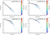 |
Fig. 5. Photospheric line indices TiO 7050 (top left panel), TiO 8430 (top right panel), VO 7436 (bottom left panel), and VO 7942 (bottom right panel) as a function of spectral type with Hα active stars coloured corresponding to their |

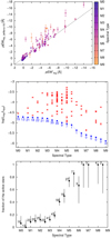 |
Fig. 6. Top panel: comparison of our |


4.3. Correlations among chromospheric lines
The spectral type dependences of our activity indicators discussed in Sect. 4.1 suggest that different chromospheric activity indicators are correlated. In this section, we test whether the chromospheric He D3, Na D, Ca IRT-a, He 10833, and Paβ lines are correlated with Hα. Using the pEW′ values derived from the co-added spectra for the 331 sample stars, we computed the Spearman correlation coefficients rS between Hα and each of the other lines as well as between He 10833 and Paβ. The corresponding scatter plots are shown in Fig. 7.
We find that He D3 is in excess emission for all stars where  Å. Because the He D3 excess emission increases linearly with further increasing Hα excess emission, we find a strong correlation with rS = 0.70. The correlation coefficient increases to rS = 0.96 when we consider only the Hα active stars. A linear correlation between these two lines was previously reported by Gizis et al. (2002). Although the flux ratio of the pseudo-continua depends on the effective temperature, we do not find a significant dependence of the slope on spectral type.
In the case of Na D, the Hα inactive stars can have excess absorption or emission with respect to the reference stars, as was described in Sect. 4.1.1. This results in an elongated cloud of data points at  Å. We find only a weak correlation with rS = 0.20 for all sample stars. For the Hα active stars, however, the excess emission in Hα and Na D is correlated with rS = 0.60. Again, we do not find a spectral type dependence.
For Ca IRT-a, we also find an elongated cloud of data points formed by the Hα inactive stars and stronger Ca IRT-a excess emission for increasing Hα excess emission in general. However, while the correlation coefficient is rS = 0.73 for all sample stars, the correlation is weaker among the Hα active stars with rS = 0.61. This is a consequence of the spectral type dependence of the slope, which we find to be steeper for earlier spectral types. To determine whether the steeper slopes are an effect of the different pseudo-continua, we estimated the continuum radiation at different spectral types by approximating the stars as blackbodies with temperature Teff from Table 2. Planck’s law yields that at the wavelength of Hα, an M0.0 star (Teff = 3850 K) has a continuum radiation of 330 W m−2 sr−1 Å−1, whereas an M4.0 star (Teff = 3200 K) has a continuum radiation of 104 W m−2 sr−1 Å−1. Therefore, the same excess energy ΔHα results in a  that is 3.17 times as large for an M4.0 star as for an M0.0 star. In contrast, the continuum radiation at the wavelength of Ca IRT-a is 335 W m−2 sr−1 Å−1 for an M0.0 star and 136 W m−2 sr−1 Å−1 for an M4.0 star. Therefore, the same excess energy ΔCa IRT-a results in a
  that is 2.46 times as high for an M4.0 star as for an M0.0 star. Consequently, a constant energy ratio ΔH α∕ΔCa IRT-a results in a pEW′ ratio that for an M4.0 star is only 0.78 times as high as for an M0.0 star. This explains the fainter slope for later spectral types that we find in the plot.
He 10833 can show excess emission or excess absorption for the Hα inactive stars. We do not see a clear correlation with  for the Hα active stars. The correlation coefficient is only rS = 0.27 for all sample stars, and rS = 0.41 for the Hα active stars. However, with increasing Hα excess emission, fewer stars have He 10833 excess absorption. There is no clear spectral type dependence.
In the case of Paβ, we find excess emission or excess absorption for the Hα inactive stars as well, no clear correlation with  for the Hα active stars, and no spectral type dependence of the correlation. Paβ excess absorption is more common in stars with
  Å, whereas more stars with stronger Hα excess emission have Paβ excess emission. The correlation coefficient is rS = −0.16 for all sample stars and rS = 0.42 for the Hα active stars. There is no strong correlation between Paβ and He 10833 either (rS = 0.26 for all sample stars, rS = 0.44 for the Hα active stars).
The correlations are in agreement with our observations in Sect. 4.1.1. Hα is correlated best with He D3, while the correlations with Na D and Ca IRT-a are weaker because the photospheric component of these lines is not completely removed by the spectral subtraction technique. The near-infrared He 10833 and Paβ lines show no strong monotonic correlation with Hα or with eachother. We do not see any clear nonmonotonic correlation, but cannot rule out that there are outliers caused by telluric linesin the integration windows of these two lines.
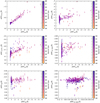 |
Fig. 7. Scatter plots of pEW′ values of Hα and He D3 (top left panel), Hα and Na D (top right panel), Hα and Ca IRT-a (centre left panel), Hα and He 10833 (centre right panel), Hα and Paβ (bottom left panel), and He 10833 and Paβ (bottom right panel). Colours denote spectral types. |
4.4. Activity effects on photospheric bands
As noted in Sect. 4.1, our photospheric TiO and VO absorption band indices show not only the expected spectral type dependence, but also a different behaviour with increasing Hα excess emission. Figure 5 shows the indices as a function of the spectral subtype, colour-coded according to  . The Hα active stars in general have lower TiO 7050 index values than the Hα inactive stars of the same spectral subtype. This effect is stronger at later spectral subtypes. Hawley et al. (1996) and Alonso-Floriano et al. (2015) reported the same behaviour for their TiO 2 index, which is comparable to our TiO 7050 index. The separation between the Hα active and Hα inactive stars appears stronger in TiO 8430, whereas no clear separation is visible in the two VO band indices.
The spectral types were derived from empirical functions of spectral indices similar to our photospheric band indices (e.g. Reid et al. 1995; Lépine et al. 2013; Alonso-Floriano et al. 2015). This means that the spectral types may be biased depending on the set of spectral indices used for the spectral type determination. In addition, spectral types are no exact quantities and the Teff ranges covered by different spectral subtypes can overlap. The direct determination of Teff, however, also uses photospheric bands like the TiO γ band at 7050 Å (Passegger et al. 2018) and may in consequence also be biased by other effects. Therefore we study the photospheric band indices only as a function of the spectral type. Because younger stars tend to be more active (Skumanich 1972; West et al. 2008), it is possible that the Hα active stars in our sample are younger and more metal rich than the Hα inactive stars, and that the differences in the photospheric band indices are caused by different metallicities. While most Hα active stars in our sample belong to the young disc or thin disc population, there are also Hα inactive stars in both populations, and we do not see any significant difference in the distribution of photospheric band indices within each population. The metallicities measured by Alonso-Floriano et al. (2015) and Passegger et al. (2018) do not show any correlation with the photospheric band indices for stars of the same spectral type either. Because population membership is only a very rough age estimate, and the metallicity measurements again are based on photospheric bands and therefore may be affected by temperature differences and other effects, we cannot rule out that the differences in the photospheric band indices of Hα active and Hα inactive stars are a metallicity effect. We do not have evidence for a metallicity effect either, however, therefore we discuss other differences between active and inactive stars that may affect the photospheric bands in the following.
One difference between active and inactive stars are active regions such as starspots. The temperature dependence of TiO bands has been used to measure starspot areas and temperatures (Neff et al. 1995; O’Neal et al. 1998). However, a lower apparent temperature of the stellar surface affects the whole spectrum and thus results in a later spectral type. Moreover, the VO band indices show a spectral-type and hence temperature dependence comparable to the TiO 8430 index for the Hα inactive stars and should thus show the same behaviour if there was a temperature change. Starspots therefore cannot explain our observations.
Another difference between active and inactive stars is the faster rotation of more active stars (e.g. Delfosse et al. 1998; Mohanty & Basri 2003; Newton et al. 2017; Jeffers et al. 2018). To investigate the effect of stellar rotation on our photospheric band indices, we applied an artificial rotational broadening to the co-added spectra of our reference stars and measured the indices in the broadened spectra. The upper panel of Fig. 8 shows the indices derived in this way for v sin i = 5 km s−1 and v sin i = 20 km s−1 divided by the indices without the rotational broadening as a function of the spectral type. While the TiO 7050 index increases with higher v sin i and this increase is larger at later spectral subtypes, the TiO 8430 index decreases with higher v sin i and the effect is smaller at later spectral subtypes. In contrast, a v sin i of 5 km s−1 has no significant effect on either VO band index and a high v sin i of 20 km s−1 increases the VO 7436 index more strongly at later spectral subtypes, whereas the VO 7942 is only affected at early spectral subtypes where no fast rotators exist in our sample. Faster rotation of more active stars can therefore explain the behaviour of the TiO 8430 and the two VO band indices, but it cannot be the only relevant effect because it results in higher TiO 7050 index values for active stars than for inactive stars, while we observe lower values.
A third difference between active and inactive stars may be stronger magnetic fields in the active stars, which lead to Zeeman broadening of the individual lines in the band. We investigated the effect of magnetic fields on the two TiO band indices using model spectra calculated for different Teff without magnetic fields and with homogeneous magnetic fields with different strengths of 2 and 4 kG. The spectra were computed with the MagneSyn magnetic spectrum synthesis code described in Shulyak et al. (2017). The transition parameters of TiO lines were extracted from the latest release of the VALD database (Ryabchikova et al. 2015). As the rotation-spin coupling constants for the VO bands are unknown, we cannot study how magnetic fields affect our VO band indices. The lower panel of Fig. 8 shows the ratio of the TiO indices of the model spectra with a magnetic field divided by the TiO indices of the model spectrum without a magnetic field for the same Teff. We find that the TiO 7050 index decreases with stronger magnetic fields and the decrease is larger at lower Teff. The TiO 8430 index also decreases with stronger magnetic fields, but this effect does not depend on Teff. The effect of Zeeman broadening on the indices is consistent with our observations.
While the TiO 8430 index is decreased by both rotational and Zeeman broadening, the TiO 7050 index is decreased by Zeeman broadening but increased by rotational broadening. This shows that a combination of both effects can explain that the observed separation between the Hα active and the Hα inactive stars of the same spectral type is stronger in the TiO 8430 index. It may also explain why the Hα active stars were not assigned later spectral subtypes, as the spectral types were derived from low-resolution spectra where the effects of rotational and Zeeman broadening may be diminished.
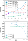 |
Fig. 8. Top panel: effect of different rotational velocities (v sin i) on the photospheric band indices as measured by the ratio of the index of the co-added spectra of the reference stars with an artificial rotational broadening to the index without rotational broadening as a function of the spectral type. Bottom panel: effect of magnetic fields on the TiO band indices as measured by the ratio of the index of model spectra with homogeneous magnetic fields of different strengths to the index of model spectra without a magnetic field for different Teff. The Teff scale is nonlinear to be consistent with the spectral type scale in the top panel. |
5. Time series of activity indicators
We now consider individual observations rather than the co-added spectra. Using the time series of the activity indicators, we investigate their variation quantitatively and examine if the variation is periodic.
5.1. Variability of activity indicators
We defined the absolute variation of each indicator as the difference between the 20th and 80th percentiles, which we calculated using the quantile estimator developed by Harrell & Davis (1982). This definition is more suitable for our data than the variance or standard deviation because occasional strong flaring events can lead to a non-normal distribution of the measured values for each star. By using the quantile estimator rather than direct percentiles, we also obtain the errors of the percentiles without assuming a specific distribution. We propagated these errors to calculate the error of the absolute variation and tabulate the results in Table A.1.
The absolute Hα variation is shown as a function of  for
for  Å in Fig. 9. While the Hα inactive stars show a mean variation of 0.07 Å in
  , the variations of the Hα active stars range between 0.10 and 8.4 Å. In particular, the stars with Hα excess emission slightly stronger than our activity threshold of
  Å show larger Hα variations than most Hα inactive stars, strengthening the choice of this threshold. It is also visible that the variations among the Hα inactive stars are larger for later spectral types. This is expected because a lower S/N leads to larger statistical fluctuations. In contrast, true variability of the stellar activity is the dominant source of Hα variations in Hα active stars because their variations are typically an order of magnitude larger than the measurement errors.
For better comparison across the different spectral types and activity levels, we divided the absolute variations by the average values as derived from the co-added spectra. The relative variations obtained in this way for Hα active stars are shown as a function of the normalised Hα luminosity in Fig. 10.
We find that the relative He D3 variation decreases with higher normalised Hα luminosity with a Spearman correlation coefficient of rS = −0.49. Two stars with log(LHα∕Lbol) < −4.0 are not shown in Fig. 10 for reasons of clarity because their 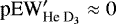 Å leads to a relative He D3 variation greater than 10. The relative Na D variation shows no clear correlation (rS = −0.24). However, as eight of nine stars with a relative Na D variation greater than 2 have a normalised Hα luminosity log(LHα∕Lbol) < −4.0, larger relative Na D variations are more common at lower activity levels.
For the relative Hα variation, we ignored one outlier caused by a poor spectrum of a star with only seven observations. With a moderate correlation coefficient of rS = −0.45, we find that more active stars show a weaker relative Hα variation, as was previously reported by Bell et al. (2012) using the standard deviation of the pEW as a measure of the variation. The anti-correlation between the relative Ca IRT-a variation and the normalised Hα luminosity is weak (rS = −0.31), but all stars with a relative Ca IRT-a variation greater than 2 have a moderate normalised Hα luminosity log(LHα∕Lbol) < −4.0. Two stars with log(LHα∕Lbol) < −4.7 have a 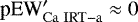 Å leading to a relative Ca IRT-a variation greater than 10, and are therefore not shown in Fig. 10.
On the whole, we find that the relative variations of He D3 and Hα are moderately anti-correlated with the normalised Hα luminosity, whereas there is only a weak anticorrelation for the relative variations of Na D and Ca IRT-a. This anti-correlation is plausible because more active stars likely have a larger number of active regions, and consequently, the effect of a single active region appearing or disappearing on the disk-integrated spectrum is lower. The weaker anti-correlation in the cases of Na D and Ca IRT-a may be a consequence of biases caused by the choice of the reference stars, as discussed in Sect. 4.1.1. The Na D variation may also be affected by telluric emission in the line window in some spectra.
We do not show the relative variations of He 10833 and Paβ because they do not show any correlation with the normalised Hα luminosity, although the spectra with telluric contamination in the He 10833 and Paβ line windows were not used to calculate the variations. The relative variations of the photospheric absorption band indices are not correlated with the normalised Hα luminosity and therefore not shown either.
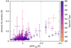 |
Fig. 9. Absolute Hα variation as defined by the difference between the 20th and 80th percentiles as a function of |


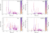 |
Fig. 10. Relative variation of chromospheric line pEW′ in Hα active stars as a function of the normalised Hα luminosity. Colours denote spectral types. Two outliers in He D3, one outlier in Hα, and two outliers in Ca IRT-a are not shown for the sake of clarity. |
5.2. Periodicities of activity indicators
In this section, we calculate periodicities of the activity indicators for the 331 stars in our sample and compare these candidate periods with known rotation periods. To remove outliers caused by flaring events or poor spectra, we rejected chromospheric line pEW′ and photospheric absorption band index values that differed from the respective average value by more than twice the standard deviation (2σ clipping). For the He 10833 and Paβ lines, we also rejected spectra with telluric contamination of the line window, as described in Sect. 3.1. We then calculated the generalised Lomb-Scargle (GLS) periodogram (Zechmeister & Kürster 2009) for each activity indicator. The best-fit frequency for each indicator is the frequency with the maximum power in the GLS periodogram. We iteratively calculated the second- and third-best-fit frequencies from the GLS periodogram of the residuals of the best-fit frequency sine curve. Since most stars were observed at most once per night, we limited our calculations to frequencies below 1 d−1. The best-fit, second-best-fit, and third-best-fit frequencies for each star and each indicator are given in Table A.1.
Long-term activity cycles in M dwarfs have been found in the range 6−7 yr (Gomes da Silva et al. 2012; Robertson et al. 2013; Suárez Mascareño et al. 2016) and therefore likely cannot be seen in our data set, which covers only 2.4 yr. However, as the star rotates, different active regions become visible over time. The activity indicators may therefore vary with the rotation period Prot, which is known for 154 stars in our sample (Kiraga & Stepien 2007; Kiraga 2012; Hunt-Walker et al. 2012; Houdebine & Mullan 2015; Suárez Mascareño et al. 2015, 2016; West et al. 2015; Newton et al. 2016; Díez Alonso et al. 2019). Of these, 133 stars have a Prot > 1 d, to which we can compare our calculated frequencies. We find 66 stars for which one of the three best-fit frequencies corresponds to Prot within three times their respective errors in at least one indicator. Some of these matches may be by chance because only for 15 of these stars Prot appears as one of the three best-fit frequencies in at least three indicators. As some active regions might disappear and new active regions might appear at different locations during the span of our observations, we cannot rule out that more stars show a semiperiodic variability of activity indicators induced by rotation over shorter time spans. However, as high-cadence observations have been conducted only for a small subset of the CARMENES sample, a period search using a shorter time baseline is beyond the scope of this paper.
For each indicator, we counted how many stars have a best-fit, second-best-fit, or third-best-fit frequency that corresponds to Prot within threetimes their respective errors. A histogram is shown in Fig. 11. We find that the TiO 7050 index varies with the rotation period most commonly, with 19 stars for which one of our three best-fit frequencies corresponds to Prot.  ,
,  , and the TiO 8430 index are the only other indicators that show Prot as one of the three best-fit frequencies for more than 10% of the 133 stars with Prot > 1 d.
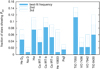 |
Fig. 11. Fraction of the 133 stars with Prot > 1 d for which the best-fit, second-best-fit, or third-best-fit frequency in the chromospheric line pEW′ or photospheric absorption band index measurements corresponds to the rotation period Prot. |
6. Summary
CARMENES searches for radial velocity variations of M dwarfs in the order of 1 m s−1 induced by planets orbiting in their liquid-water habitable zones. In this work, we have measured pseudo-equivalent widths of the He D3, Na D, Hα, Ca IRT, He 10833, and Paβ lines for 331M dwarfs using a spectral subtraction technique. Additionally, we measured indices of two photospheric TiO and two photospheric VO absorption bands. Our results improve our understanding of stellar activity in the CARMENES sample of M dwarfs.
We used the stars with the longest known rotation period as reference stars for each spectral subtype and found no stars with considerably stronger Hα absorption than these reference stars. This implies that all our sample stars have at least a minimum level of chromospheric inactivity because we would expect to measure stronger Hα excess absorption at low activity levels if the reference star had a completely inactive chromosphere (Cram & Mullan 1979). We defined stars with  Å as Hα active and found that 29% of our sample stars are Hα active. The fraction of Hα active stars is below 20% for spectral subtype M3.5 V and earlier and significantly increases at later spectral subtypes. In addition, the normalised Hα luminosity of typical Hα active stars increases with spectral subtype up to M5.0 V. This confirms the results of previous M dwarf activity studies by Reiners et al. (2012), West et al. (2015), and Jeffers et al. (2018).
We showed that the He D3 line is strongly correlated with Hα, as was previously reported by Gizis et al. (2002). The Na D doublet and the Ca IRT show a weaker correlation because their photospheric components are too different for stars of the same spectral subtype and are therefore not completely removed by our spectral subtraction technique. He 10833 and Paβ are challenging to measure because of telluric contamination and because they are not clearly correlated with the other indicators. The unclear correlation suggests that the He 10833 line is not very sensitive to activity, and this increases its usefulness as a tracer of exoplanet atmospheres (e.g. Spake et al. 2018; Nortmann et al. 2018; Salz et al. 2018).
We found that the photospheric TiO 7050 and TiO 8430 indices of Hα active stars have lower values than the indices of Hα inactive stars of the same spectral subtype. The VO 7436 and VO 7942 indices do not show this separation. We showed that this behaviour can be explained by rotational and Zeeman broadening, which are stronger in active stars.
We quantified the variation of the activity indicators for all stars in the sample. In units of the respective pEW′ as derived from co-added spectra, the variations in the Hα and He D3 lines among multiple observations are smaller for more active stars. The anti-correlation between the normalised Hα luminosity and the relative variations in Na D and Ca IRT-a lines is weaker, whereas the variations in He 10833 and Paβ show no correlation.
We calculated periodicities in the activity indicators of each star using GLS periodograms and compared the three best-fit frequencies with known rotation periods Prot. The TiO 7050 index,  ,
,  , and the TiO 8430 are most likely to vary with the rotation period. Of the 133 stars with Prot > 1 d, 66 show the rotation period in at least one activity indicator. Because the other 67 stars could show the rotation period in the activity indicators during parts of the time baseline, a semi-periodic activity variation of a different origin might not be present all the time either. However, this semi-periodic variation could still lead to periodic changes in the measured radial velocity, which might be misinterpreted as induced by a planet. Only 15 stars show the rotation period in at least three activity indicators. A careful study of individual stars is necessary to understand why the rotation period may appear in some but not all indicators, but this is beyond the scope of this paper, which is focused on the full CARMENES sample.
Acknowledgements
CARMENES is an instrument for the Centro Astronómico Hispano-Alemán de Calar Alto (CAHA, Almería, Spain). CARMENES is funded by the German Max-Planck-Gesellschaft (MPG), the Spanish Consejo Superior de Investigaciones Científicas (CSIC), the European Union through FEDER/ERF FICTS-2011-02 funds, and the members of the CARMENES Consortium (Max-Planck-Institut für Astronomie, Instituto de Astrofísica de Andalucía, Landessternwarte Königstuhl, Institut de Ciències de l’Espai, Institut für Astrophysik Göttingen, Universidad Complutense de Madrid, Thüringer Landessternwarte Tautenburg, Instituto de Astrofísica de Canarias, Hamburger Sternwarte, Centro de Astrobiología and Centro Astronómico Hispano-Alemán), with additional contributions by the Spanish Ministry of Science, the German Science Foundation through the Major Research Instrumentation Programme and DFG Research Unit FOR2544 “Blue Planets around Red Stars”, the Klaus Tschira Stiftung, the states of Baden-Württemberg and Niedersachsen, and by the Junta de Andalucía.
Appendix A: Table of results
Identification, common name, Gliese number, spectral type (SpT), stellar population (Pop.), rotational velocity, rotation period, normalised Hα luminosity,  , absolute Hα variation, andthe three best-fit frequencies for Hα.
References
- Aigrain, S., Pont, F., & Zucker, S. 2012, MNRAS, 419, 3147 [NASA ADS] [CrossRef] [Google Scholar]
- Alonso-Floriano, F. J., Morales, J. C., Caballero, J. A., et al. 2015, A&A, 577, A128 [NASA ADS] [CrossRef] [EDP Sciences] [Google Scholar]
- Baliunas, S. L., Donahue, R. A., Soon, W. H., et al. 1995, ApJ, 438, 269 [NASA ADS] [CrossRef] [Google Scholar]
- Barnes, J. R., Jenkins, J. S., Jones, H. R. A., et al. 2014, MNRAS, 439, 3094 [NASA ADS] [CrossRef] [Google Scholar]
- Baroch, D., Morales, J. C., Ribas, I., et al. 2018, A&A, 619, A32 [NASA ADS] [CrossRef] [EDP Sciences] [Google Scholar]
- Bell, K. J., Hilton, E. J., Davenport, J. R. A., et al. 2012, PASP, 124, 14 [NASA ADS] [CrossRef] [Google Scholar]
- Benneke, B., Werner, M., Petigura, E., et al. 2017, ApJ, 834, 187 [NASA ADS] [CrossRef] [Google Scholar]
- Berdyugina, S. V., & Solanki, S. K. 2002, A&A, 385, 701 [NASA ADS] [CrossRef] [EDP Sciences] [Google Scholar]
- Bessell, M. S. 1982, PASA, 4, 417 [NASA ADS] [CrossRef] [Google Scholar]
- Cortés-Contreras, M. 2016, Ph.D. Thesis, Universidad Complutense de Madrid, Spain [Google Scholar]
- Cortés-Contreras, M., Béjar, V. J. S., Caballero, J. A., et al. 2017, A&A, 597, A47 [NASA ADS] [CrossRef] [EDP Sciences] [Google Scholar]
- Covey, K. R., Ivezić, Ž., Schlegel, D., et al. 2007, AJ, 134, 2398 [NASA ADS] [CrossRef] [Google Scholar]
- Cram, L. E., & Mullan, D. J. 1979, ApJ, 234, 579 [NASA ADS] [CrossRef] [EDP Sciences] [Google Scholar]
- David, T. J., Hillenbrand, L. A., Petigura, E. A., et al. 2016, Nature, 534, 658 [NASA ADS] [CrossRef] [PubMed] [Google Scholar]
- Davison, C. L., White, R. J., Henry, T. J., et al. 2015, AJ, 149, 106 [NASA ADS] [CrossRef] [Google Scholar]
- Delfosse, X., Forveille, T., Perrier, C., & Mayor, M. 1998, A&A, 331, 581 [NASA ADS] [Google Scholar]
- Díez Alonso, E., Caballero, J. A., Montes, D., et al. 2019, A&A, 621, A126 [NASA ADS] [CrossRef] [EDP Sciences] [Google Scholar]
- Gaidos, E., Mann, A. W., Lépine, S., et al. 2014, MNRAS, 443, 2561 [NASA ADS] [CrossRef] [Google Scholar]
- Gigoyan, K. S., Sinamyan, P. K., Engels, D., & Mickaelian, A. M. 2010, Astrophysics, 53, 123 [NASA ADS] [CrossRef] [Google Scholar]
- Gizis, J. E., Reid, I. N., & Hawley, S. L. 2002, AJ, 123, 3356 [NASA ADS] [CrossRef] [Google Scholar]
- Gomes da Silva, J., Santos, N. C., Bonfils, X., et al. 2012, A&A, 541, A9 [NASA ADS] [CrossRef] [EDP Sciences] [Google Scholar]
- Gray, R. O., Corbally, C. J., Garrison, R. F., McFadden, M. T., & Robinson, P. E. 2003, AJ, 126, 2048 [NASA ADS] [CrossRef] [Google Scholar]
- Gray, R. O., Corbally, C. J., Garrison, R. F., et al. 2006, AJ, 132, 161 [NASA ADS] [CrossRef] [Google Scholar]
- Harrell, F. E., & Davis, C. E. 1982, Biometrika, 69, 635 [Google Scholar]
- Hawley, S. L., Gizis, J. E., & Reid, I. N. 1996, AJ, 112, 2799 [NASA ADS] [CrossRef] [Google Scholar]
- Hawley, S. L., Covey, K. R., Knapp, G. R., et al. 2002, AJ, 123, 3409 [NASA ADS] [CrossRef] [Google Scholar]
- Hirano, T., Dai, F., Livingston, J. H., et al. 2018, AJ, 155, 124 [NASA ADS] [CrossRef] [Google Scholar]
- Houdebine, E. R., & Mullan, D. J. 2015, ApJ, 801, 106 [NASA ADS] [CrossRef] [Google Scholar]
- Houdebine, E. R., Junghans, K., Heanue, M. C., & Andrews, A. D. 2009, A&A, 503, 929 [NASA ADS] [CrossRef] [EDP Sciences] [Google Scholar]
- Hunt-Walker, N. M., Hilton, E. J., Kowalski, A. F., Hawley, S. L., & Matthews, J. M. 2012, PASP, 124, 545 [Google Scholar]
- Jeffers, S. V., Schöfer, P., Lamert, A., et al. 2018, A&A, 614, A76 [NASA ADS] [CrossRef] [EDP Sciences] [Google Scholar]
- Jenkins, J. S., Ramsey, L. W., Jones, H. R. A., et al. 2009, ApJ, 704, 975 [NASA ADS] [CrossRef] [Google Scholar]
- Jones, J. E., Alloin, D. M., & Jones, B. J. T. 1984, ApJ, 283, 457 [NASA ADS] [CrossRef] [Google Scholar]
- Jorgensen, U. G., Carlsson, M., & Johnson, H. R. 1992, A&A, 254, 258 [NASA ADS] [Google Scholar]
- Kiraga, M. 2012, Acta Astron., 62, 67 [NASA ADS] [Google Scholar]
- Kiraga, M., & Stepien, K. 2007, Acta Astron., 57, 149 [NASA ADS] [Google Scholar]
- Kirkpatrick, J. D., Henry, T. J., & McCarthy, Jr. D. W. 1991, ApJS, 77, 417 [NASA ADS] [CrossRef] [Google Scholar]
- Kirkpatrick, J. D., Kelly, D. M., Rieke, G. H., et al. 1993, ApJ, 402, 643 [NASA ADS] [CrossRef] [Google Scholar]
- Kirkpatrick, J. D., Reid, I. N., Liebert, J., et al. 1999, ApJ, 519, 802 [NASA ADS] [CrossRef] [Google Scholar]
- Lépine, S., Rich, R. M., & Shara, M. M. 2003, AJ, 125, 1598 [NASA ADS] [CrossRef] [Google Scholar]
- Lépine, S., Rich, R. M., & Shara, M. M. 2007, ApJ, 669, 1235 [NASA ADS] [CrossRef] [Google Scholar]
- Lépine, S., Hilton, E. J., Mann, A. W., et al. 2013, AJ, 145, 102 [NASA ADS] [CrossRef] [Google Scholar]
- Luyten, W. J. 1923, PASP, 35, 175 [NASA ADS] [CrossRef] [Google Scholar]
- Mallik, S. V. 1997, A&AS, 124, 359 [NASA ADS] [CrossRef] [EDP Sciences] [Google Scholar]
- Martín, E. L., Delfosse, X., Basri, G., et al. 1999, AJ, 118, 2466 [NASA ADS] [CrossRef] [Google Scholar]
- Martin, J., Fuhrmeister, B., Mittag, M., et al. 2017, A&A, 605, A113 [NASA ADS] [CrossRef] [EDP Sciences] [Google Scholar]
- Mohanty, S., & Basri, G. 2003, ApJ, 583, 451 [NASA ADS] [CrossRef] [Google Scholar]
- Montes, D., Fernandez-Figueroa, M. J., de Castro, E., & Cornide, M. 1995, A&A, 294, 165 [NASA ADS] [Google Scholar]
- Montes, D., López-Santiago, J., Gálvez, M. C., et al. 2001, MNRAS, 328, 45 [NASA ADS] [CrossRef] [MathSciNet] [Google Scholar]
- Neff, J. E., O’Neal, D., & Saar, S. H. 1995, ApJ, 452, 879 [NASA ADS] [CrossRef] [Google Scholar]
- Newton, E. R., Charbonneau, D., Irwin, J., et al. 2014, AJ, 147, 20 [NASA ADS] [CrossRef] [Google Scholar]
- Newton, E. R., Irwin, J., Charbonneau, D., et al. 2016, ApJ, 821, 93 [NASA ADS] [CrossRef] [Google Scholar]
- Newton, E. R., Irwin, J., Charbonneau, D., et al. 2017, ApJ, 834, 85 [NASA ADS] [CrossRef] [Google Scholar]
- Nortmann, L., Pallé, E., Salz, M., et al. 2018, Science, 362, 1388 [NASA ADS] [CrossRef] [EDP Sciences] [Google Scholar]
- O’Neal, D., Neff, J. E., & Saar, S. H. 1998, ApJ, 507, 919 [NASA ADS] [CrossRef] [Google Scholar]
- Passegger, V. M., Reiners, A., Jeffers, S. V., et al. 2018, A&A, 615, A6 [NASA ADS] [CrossRef] [EDP Sciences] [Google Scholar]
- Pecaut, M. J., & Mamajek, E. E. 2013, ApJS, 208, 9 [NASA ADS] [CrossRef] [Google Scholar]
- Pineda, J. S., West, A. A., Bochanski, J. J., & Burgasser, A. J. 2013, AJ, 146, 50 [NASA ADS] [CrossRef] [Google Scholar]
- Queloz, D., Henry, G. W., Sivan, J. P., et al. 2001, A&A, 379, 279 [NASA ADS] [CrossRef] [EDP Sciences] [Google Scholar]
- Quirrenbach, A., Amado, P. J., Ribas, I., et al. 2018, in Ground-based and Airborne Instrumentation for Astronomy VII, SPIE Conf. Ser., 10702, 107020W [Google Scholar]
- Reid, I. N., Hawley, S. L., & Gizis, J. E. 1995, AJ, 110, 1838 [NASA ADS] [CrossRef] [Google Scholar]
- Reiners, A., & Basri, G. 2008, ApJ, 684, 1390 [NASA ADS] [CrossRef] [Google Scholar]
- Reiners, A., & Basri, G. 2010, ApJ, 710, 924 [NASA ADS] [CrossRef] [Google Scholar]
- Reiners, A., Joshi, N., & Goldman, B. 2012, AJ, 143, 93 [NASA ADS] [CrossRef] [Google Scholar]
- Reiners, A., Zechmeister, M., Caballero, J. A., et al. 2018, A&A, 612, A49 [NASA ADS] [CrossRef] [EDP Sciences] [Google Scholar]
- Riaz, B., Gizis, J. E., & Harvin, J. 2006, AJ, 132, 866 [NASA ADS] [CrossRef] [Google Scholar]
- Riedel, A. R., Finch, C. T., Henry, T. J., et al. 2014, AJ, 147, 85 [NASA ADS] [CrossRef] [Google Scholar]
- Robertson, P., Endl, M., Cochran, W. D., & Dodson-Robinson, S. E. 2013, ApJ, 764, 3 [NASA ADS] [CrossRef] [Google Scholar]
- Robertson, P., Bender, C., Mahadevan, S., Roy, A., & Ramsey, L. W. 2016, ApJ, 832, 112 [NASA ADS] [CrossRef] [Google Scholar]
- Ryabchikova, T., Piskunov, N., Kurucz, R. L., et al. 2015, Phys. Scr, 90, 054005 [NASA ADS] [CrossRef] [Google Scholar]
- Salz, M., Czesla, S., Schneider, P. C., et al. 2018, A&A, 620, A97 [NASA ADS] [CrossRef] [EDP Sciences] [Google Scholar]
- Sanz-Forcada, J., & Dupree, A. K. 2008, A&A, 488, 715 [NASA ADS] [CrossRef] [EDP Sciences] [Google Scholar]
- Schmidt, S. J., Cruz, K. L., Bongiorno, B. J., Liebert, J., & Reid, I. N. 2007, AJ, 133, 2258 [NASA ADS] [CrossRef] [Google Scholar]
- Schmidt, S. J., Kowalski, A. F., Hawley, S. L., et al. 2012, ApJ, 745, 14 [NASA ADS] [CrossRef] [Google Scholar]
- Scholz, R.-D., Meusinger, H., & Jahreiß, H. 2005, A&A, 442, 211 [NASA ADS] [CrossRef] [EDP Sciences] [Google Scholar]
- Shkolnik, E., Liu, M. C., & Reid, I. N. 2009, ApJ, 699, 649 [NASA ADS] [CrossRef] [Google Scholar]
- Shkolnik, E. L., Hebb, L., Liu, M. C., Reid, I. N., & Collier Cameron, A. 2010, ApJ, 716, 1522 [NASA ADS] [CrossRef] [Google Scholar]
- Short, C. I., & Doyle, J. G. 1998, A&A, 331, L5 [NASA ADS] [Google Scholar]
- Shulyak, D., Reiners, A., Engeln, A., et al. 2017, Nat. Astron., 1, 0184 [NASA ADS] [CrossRef] [Google Scholar]
- Skumanich, A. 1972, ApJ, 171, 565 [NASA ADS] [CrossRef] [Google Scholar]
- Spake, J. J., Sing, D. K., Evans, T. M., et al. 2018, Nature, 557, 68 [NASA ADS] [CrossRef] [EDP Sciences] [Google Scholar]
- Spinrad, H. 1962, ApJ, 135, 715 [NASA ADS] [CrossRef] [Google Scholar]
- Stassun, K. G., Hebb, L., Covey, K., et al. 2011, in 16th Cambridge Workshop on Cool Stars, Stellar Systems, and the Sun, eds. C. Johns-Krull, M. K. Browning, & A. A. West, ASP Conf. Ser., 448, 505 [NASA ADS] [Google Scholar]
- Stauffer, J. R., & Hartmann, L. W. 1986, ApJS, 61, 531 [NASA ADS] [CrossRef] [Google Scholar]
- Suárez Mascareño, A., Rebolo, R., González Hernández, J. I., & Esposito, M. 2015, MNRAS, 452, 2745 [NASA ADS] [CrossRef] [Google Scholar]
- Suárez Mascareño, A., Rebolo, R., & González Hernández, J. I. 2016, A&A, 595, A12 [NASA ADS] [CrossRef] [EDP Sciences] [Google Scholar]
- Vollmann, K., & Eversberg, T. 2006, Astron. Nachr., 327, 862 [NASA ADS] [CrossRef] [Google Scholar]
- Walkowicz, L. M., Hawley, S. L., & West, A. A. 2004, PASP, 116, 1105 [NASA ADS] [CrossRef] [Google Scholar]
- West, A. A., Hawley, S. L., Walkowicz, L. M., et al. 2004, AJ, 128, 426 [NASA ADS] [CrossRef] [Google Scholar]
- West, A. A., Hawley, S. L., Bochanski, J. J., et al. 2008, AJ, 135, 785 [NASA ADS] [CrossRef] [Google Scholar]
- West, A. A., Morgan, D. P., Bochanski, J. J., et al. 2011, AJ, 141, 97 [NASA ADS] [CrossRef] [Google Scholar]
- West, A. A., Weisenburger, K. L., Irwin, J., et al. 2015, ApJ, 812, 3 [NASA ADS] [CrossRef] [Google Scholar]
- Wilson, O. C. 1968, ApJ, 153, 221 [NASA ADS] [CrossRef] [Google Scholar]
- Young, A., Skumanich, A., Stauffer, J. R., Harlan, E., & Bopp, B. W. 1989, ApJ, 344, 427 [NASA ADS] [CrossRef] [Google Scholar]
- Zechmeister, M., & Kürster, M. 2009, A&A, 496, 577 [NASA ADS] [CrossRef] [EDP Sciences] [Google Scholar]
- Zechmeister, M., Anglada-Escudé, G., & Reiners, A. 2014, A&A, 561, A59 [NASA ADS] [CrossRef] [EDP Sciences] [Google Scholar]
- Zechmeister, M., Reiners, A., Amado, P. J., et al. 2018, A&A, 609, A12 [CrossRef] [Google Scholar]
- Zirin, H. 1982, ApJ, 260, 655 [NASA ADS] [CrossRef] [Google Scholar]
All Tables
Integration windows and pseudo-continuum ranges for pEW’ measurements of the selected lines that are sensitive to chromospheric activity.
Identification, common name, Gliese number, spectral type (SpT), stellar population (Pop.), rotational velocity, rotation period, normalised Hα luminosity, , absolute Hα variation, andthe three best-fit frequencies for Hα.
All Figures
|
Fig. 1. Hα region in the co-added spectra of the slow-rotating, Hα inactive reference stars given in Table 2. |
| In the text | |
|
Fig. 2. Selected spectra in regions around the considered chromospheric lines: an inactive M0.0 star (J14257+236W, black), a moderately active M2.0 star (J18174+483, purple), a very active M3.5 star (J22468+443) in flaring (green) and quiescent state (blue), and a moderately active M7.0 star (J02530+168, orange). The region around the He D3 and Na D lines (top left panel) in the M7.0 spectrum is not shown because of a low signal-to-noise ratio. Bars mark the line windowranges (solid) and pseudo-continuum ranges (dashed) as given in Table 1. In the case of Hα, we also show the line window and pseudo-continuum ranges used by Jeffers et al. (2018; red) and by Reid et al. (1995) and Alonso-Floriano et al. (2015; blue). |
| In the text | |
|
Fig. 3. Same spectra as in Fig. 2 in regions around the considered photospheric bands. Bars mark the numerator ranges (solid) and denominator ranges (dashed) as given in Table 3. |
| In the text | |
|
Fig. 4. pEW′ of chromospheric lines as a function of spectral type. |
| In the text | |
|
Fig. 5. Photospheric line indices TiO 7050 (top left panel), TiO 8430 (top right panel), VO 7436 (bottom left panel), and VO 7942 (bottom right panel) as a function of spectral type with Hα active stars coloured corresponding to their |
| In the text | |
|
Fig. 6. Top panel: comparison of our |
| In the text | |
|
Fig. 7. Scatter plots of pEW′ values of Hα and He D3 (top left panel), Hα and Na D (top right panel), Hα and Ca IRT-a (centre left panel), Hα and He 10833 (centre right panel), Hα and Paβ (bottom left panel), and He 10833 and Paβ (bottom right panel). Colours denote spectral types. |
| In the text | |
|
Fig. 8. Top panel: effect of different rotational velocities (v sin i) on the photospheric band indices as measured by the ratio of the index of the co-added spectra of the reference stars with an artificial rotational broadening to the index without rotational broadening as a function of the spectral type. Bottom panel: effect of magnetic fields on the TiO band indices as measured by the ratio of the index of model spectra with homogeneous magnetic fields of different strengths to the index of model spectra without a magnetic field for different Teff. The Teff scale is nonlinear to be consistent with the spectral type scale in the top panel. |
| In the text | |
|
Fig. 9. Absolute Hα variation as defined by the difference between the 20th and 80th percentiles as a function of |
| In the text | |
|
Fig. 10. Relative variation of chromospheric line pEW′ in Hα active stars as a function of the normalised Hα luminosity. Colours denote spectral types. Two outliers in He D3, one outlier in Hα, and two outliers in Ca IRT-a are not shown for the sake of clarity. |
| In the text | |
|
Fig. 11. Fraction of the 133 stars with Prot > 1 d for which the best-fit, second-best-fit, or third-best-fit frequency in the chromospheric line pEW′ or photospheric absorption band index measurements corresponds to the rotation period Prot. |
| In the text | |
Current usage metrics show cumulative count of Article Views (full-text article views including HTML views, PDF and ePub downloads, according to the available data) and Abstracts Views on Vision4Press platform.
Data correspond to usage on the plateform after 2015. The current usage metrics is available 48-96 hours after online publication and is updated daily on week days.
Initial download of the metrics may take a while.