© R. Z. Ferret 2019

1. Introduction

Observations of supergranulation at the solar surface show it as a distinct cellular pattern of horizontal diverging flows separated by regions of convergence. Hart (1954) observed supergranulation for the first time. Leighton et al. (1962) and Simon & Leighton (1964) characterized it in the following decade. Rieutord & Rincon (2010) presented a detailed review of supergranulation.

Today, the surface properties of supergranulation are well studied. Using f-mode helioseismology, Duvall & Gizon (2000) showed that the horizontal scales of supergranulation range from about 20 to 70 Mm at the photosphere with an average size of 30 Mm, corroborating the findings of Hathaway et al. (2000). Supergranules have a typical lifespan of one to two days (see, e.g., Hirzberger et al. 2008). However, individual cells have been observed to live for longer than a week (Gizon 2006). Finally, supergranules are characterized by a horizontal surface flow of about 300 m s⁻¹ rms (Hathaway et al. 2002; Rieutord et al. 2010) and a much slower vertical surface flow of 10–30 m s⁻¹ at the center of the cell (Hathaway et al. 2002; Duvall & Birch 2010).

The properties of supergranules below the visible surface remain an open question. Many helioseismic studies of supergranulation use separable models in 2D cylindrical-polar coordinates to attempt to derive the subsurface characteristics of supergranules. A flow is separable in any coordinate system (x₁, x₂) if the components can be written as

$$\begin{array}{cc}\hfill v_1(x_1,x_2)& =f(x_1)g(x_2),\hfill \\ \hfill v_2(x_1,x_2)& =p(x_1)q(x_2).\hfill \end{array}$$(1)

Because of this property, separable models tend to simplify problems involving inversions, which are common in helioseismology.

Comparing travel-times obtained using the ray approximation on a separable flow model with helioseismic observations, Duvall & Hanasoge (2013) argued that supergranulation is a shallow process, the vertical velocity of which is highest at 2–3 Mm below the surface. However, DeGrave & Jackiewicz (2015) compared the separable flow model from Duvall & Hanasoge (2013) with helioseismic observations of an average supergranule. These latter authors derived the horizontal structure of the observed average supergranule at different depths from inversions of HMI travel-time maps and found that the model predictions of velocities were much larger (up to an order of magnitude) than the observed velocities. They claim to observe a weak horizontal inflow up to 20 Mm in depth, in contrast with the shallow supergranules predicted by Duvall & Hanasoge (2013).

A model akin to that described by Duvall & Hanasoge (2013) was used in Dombroski et al. (2013) to test a regularized least-squares inversion of helioseismic observations of supergranular flows. Instead of modeling the vertical variation of the vertical velocity by a Gaussian, as is described by Duvall & Hanasoge (2013), Dombroski et al. (2013) model the vertical variation of the horizontal velocity by a sum of Gaussian contributions corresponding to the outflow (top of the cell) and inflow (bottom of the cell). The horizontal variation is the same as in Duvall & Hanasoge (2013). Bhattacharya et al. (2017) developed a 2D helioseismic inversion algorithm that could retrieve properties of a similar separable flow model up to depths of 8–10 Mm without noise. This method has not yet been applied to observations.

In this paper we test the ability of mass-conserving flow models that are separable in the spherical-polar coordinates of the problem to reproduce photospheric observations of an average supergranule. The average supergranule is obtained by averaging the velocity maps of ∼10⁴ supergranules. This averaging process includes different horizontal scales. It is reasonable to expect that the vertical length scale of a supergranule is correlated with its horizontal length scale. Therefore one might presume that separable models are incompatible with this average. In a second experiment, we select the horizontal scales included in the averaging process to establish whether nonseparability is inherent to supergranulation or is due to the multiple scales included in the observations.

This paper uses photospheric observations from the Helioseismic and Magnetic Imager (HMI, Schou et al. 2012) on board the Solar Dynamics Observatory spacecraft (SDO, Pesnell et al. 2012). Section 2 introduces the photospheric velocity fields for an average supergranule derived from the HMI observations as well as the associated error estimates. We formulate the hypotheses of mass conservation and separable models in Sect. 3. Section 4 discusses the compatibility of separable models with observations under the given hypotheses. This latter section also investigates the influence of the averaging over different scales on the resulting incompatibility. We present our conclusions in Sect. 5.

2. Observations of supergranular flows at the surface

2.1. Geometry of the problem

We consider a spherical-polar geometry (see Fig. 1) that is more adapted to the geometry of the Sun than a cylindrical-polar coordinate system. The radius is r (r = R_⊙ at the solar surface with R_⊙ ≃ 696 Mm and r = 0 at the center of the Sun) and θ is the heliocentric angular distance from the center of the supergranule. The quantity θR_⊙ is the distance measured along the surface from the center of the supergranule. The problem is assumed to be axisymmetric.

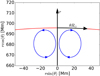Fig. 1. Geometry of the problem. The black arrows show the unitary coordinate vectors. The center of the coordinate system coincides with the center of the Sun. The coordinate r is the radius (r = R⊙ at the photosphere shown in red) and θ is the heliocentric angular distance from the center of the supergranule. Hypothetical supergranular flows are shown in blue.

In this coordinate system, Eq. (1) is

$$\begin{array}{cc}\hfill v_{\theta }(r,\theta )& =f(r)g(\theta ),\hfill \\ \hfill v_{\mathrm{r}}(r,\theta )& =p(r)q(\theta ).\hfill \end{array}$$(2)

2.2. The “average supergranule”

This study confronts observations of the velocity components for an average supergranule with the hypothesis of separability in r and θ coordinates. The observations used in this paper come from Langfellner et al. (2015a). This section explains how they obtain an average supergranule from velocity maps derived from one year of SDO/HMI observations (from 01.05.2010 to 30.04.2011).

Velocity maps were obtained from surface observations (Dopplergrams for the vertical velocity, intensity images for the horizontal velocity) centered at the equator. Image patches of approximate size 180 × 180 Mm² were remapped using Postel’s projection and tracked for 8 h (in contrast to 24 h in Langfellner et al. 2015a) as they cross the central meridian. The tracking rate is the surface equatorial solar rotation rate from Snodgrass (1984). This results in 365 eight-hour data cubes whose centers cross the central meridian halfway through the tracking period.

Observations that have a low duty cycle (<90%) or visible activity (maximum absolute intensity contrast >10%) were discarded. This reduces the total number of eight-hour sets from 365 to 326.

Langfellner et al. (2015a) identified the position of each individual supergranule on surface velocity maps using f-mode divergence sensitive travel times (“outwards minus inwards” travel-times, see Duvall et al. 1996). One full year of line-of-sight Doppler images taken by SDO/HMI near disk center as they cross the central meridian were used as an input for the travel-time computation. Figure 2 shows an example travel-time map with individual supergranules identified as green crosses. The supergranule boundaries are identified using the image segmentation algorithm described by Hirzberger et al. (2008) and the center of a supergranule is located at the maximum divergence.

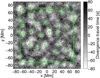Fig. 2. Identification of supergranules (green crosses) in an example 8 h map of divergence-sensitive f-mode travel times computed at the equator, near disk center, using the method in Langfellner et al. (2015a). The x coordinate is in the east-west direction (positive towards west), the y coordinate is in the north-south direction (positive towards north). The gray-scale indicates the value of the divergence-sensitive travel times from which we derive the position of the supergranules. White indicates outflows, black inflows.

The authors copy and shift each map so that the center of the selected supergranule coincides with the center of the grid. They discard supergranules located less than 18 Mm away from the edges of the map (in contrast to 8 Mm in Langfellner et al. 2015a).

A total of ∼10⁴ individual supergranules are then stacked up and averaged to reduce the noise. The vertical velocity component derived from Doppler observations is v_r and v_θ is the horizontal velocity component derived from LCT observations. The following sections detail how the velocity fields are obtained from observations.

2.3. Vertical velocity from Doppler observations

The Doppler observations are averaged over eight-hour time intervals, then the mean map over all data cubes is removed from each individual eight-hour data set. This ensures that most of the background velocity (from differential rotation, larger-scale convection, etc.) is not included in the final Doppler observations. The resulting velocity maps are 2D in Cartesian coordinates with x being the east-west direction (directed westwards) and y the north-south direction (directed northwards).

The supergranules are equally distributed in the east-west direction around the central meridian and the north-south direction around the equator. As a result, the leakage of the horizontal velocity field into the Doppler observations mostly cancels out during the averaging and we can approximate the Doppler observations to be the vertical velocity for the average supergranule.

We assume the resulting observed velocity v_D(x, y) to be

$$\begin{array}{c}\hfill v_{\mathrm{D}}(x,y)={\displaystyle \int W_{\mathrm{D}}(r)v_r(x,y,r)}\mathrm{d}r,\end{array}$$(3)

where v_r is the vertical component of velocity in the solar interior and atmosphere and W_D is the Doppler response function. The integral spans all radii.

Fleck et al. (2011) determined that the observed Doppler velocities were consistent with the velocity response function for the center of gravity of the spectral line used by HMI. Bello González et al. (2009) computed this response function. We approximate the velocity response function shown in Fig. 2 of Bello González et al. (2009) by a Gaussian that is normalized such that ∫W_D(r) dr = 1. The Gaussian peaks at R_D = 100 km above the surface and has a FWHM of 240 km. This approximation does not influence the rest of our analysis in this paper, as discussed in Sect. 3.2.

2.4. Horizontal velocity from local correlation tracking of granules

Langfellner et al. (2015a) apply local correlation tracking (LCT, the method is described by November & Simon 1988) to the previously described 326 eight-hour patches of intensity images taken by SDO/HMI. The LCT method cross-correlates small regions from pairs of consecutive images which are separated by a time lag of 45 s. From shifts in the spatial cross-correlation, they infer the advection of the granules due to larger-scale flows.

We model the granulation tracking data by a vertical average of the horizontal velocity component:

$$\begin{array}{c}\hfill {\mathit{v}}_{\mathrm{LCT}}(x,y)={\displaystyle \int W_{\mathrm{LCT}}(r){\mathit{v}}_{\mathrm{h}}(x,y,r)}\mathrm{d}r.\end{array}$$(4)

The function W_LCT(r) is the weighting function associated with LCT observations.

The equivalent of a response function for the LCT measurements is not available. Instead, we approximate the “response function” by a skewed Gaussian peaking at 100 km below the surface. The LCT measurements are based on granule tracking (Rieutord et al. 2001) and granules do not extend above the surface. Therefore we choose the skewness parameter so that the weighting function is only sensitive to velocities below the surface. This choice does not impact the main conclusion of the paper, as discussed in Sect. 3.2.

In practice:

$$\begin{array}{c}\hfill W_{\mathrm{LCT}}(r)=Aexp(-\frac{{(r-R_{\odot }-R_{\mathrm{LCT}})}^2}{2{\sigma }_{\mathrm{LCT}}^2})(1-\mathrm{erf}\left(\frac{(r-R_{\odot })}{D}\right)),\end{array}$$(5)

where A is chosen so that ∫W_LCT(r) dr = 1 and R_LCT = −0.100 Mm, σ_LCT such that the FWHM is 0.200 Mm, $D=\sqrt{2}\times 10$ km. The function erf is the error function as defined by Abramowitz & Stegun (1965). Figure 3 shows the W_LCT used in this paper.

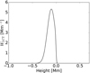Fig. 3. Assumed weighting function WLCT (see Eq. (5)) as a function of height with the parameters used in this paper.

2.5. Surface velocity components of the average supergranule

Figure 4 shows the horizontal and vertical velocity fields for an average supergranule at the surface in Cartesian coordinates. The center of the map coincides with the center of the supergranule.

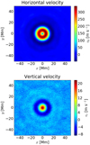Fig. 4. Horizontal (top panel) and vertical (bottom panel) components of the velocity at the surface. The x coordinate is in the east-west direction (pointed westwards), the y coordinate is in the north-south direction (pointed northwards). The maps are centered at the center of the supergranule. Red indicates outflows (horizontal component) and upflows (vertical component).

The velocity maps are averaged along the azimuthal direction to obtain the velocity fields for an average supergranule depending only on the horizontal distance from the center of the cell. Because Postel’s projection preserves distance from the center of the map, θR_⊙ is equivalent to $\sqrt{x^2+{\mathit{y}}^2}$. Supergranules are not exactly azimuthally symmetrical (Langfellner et al. 2015b); however, the departure from symmetry is small and can be ignored as a first approximation.

Figure 5 (top panel) shows the velocity components v_r and v_θ as functions of θR_⊙. These velocity components correspond to outflows. The horizontal component is ten times larger in amplitude than the vertical component, which is consistent with values found in the literature. Most of the signal is concentrated in the first 20 Mm from the center of the supergranule and becomes indistinguishable from noise at about 50 Mm from the center.

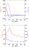Fig. 5. Top panel: observed vertical velocity vr (blue curve) and horizontal velocity vθ (red curve) for an average supergranule as a function of the surface distance θR⊙ from the center of the supergranule. Bottom panel: error estimates on the LCT observations (red curve) and Doppler observations (blue curve).

2.6. Error estimates

To compute the sample standard deviation, Langfellner et al. (2015a) derive the velocity components for each of the 326 resulting eight-hour sets and compute the variance between the 326 velocity curves for both components. The square root of the variance divided by the square root of the number of data cubes is the sample standard deviation of the horizontal and vertical components (σ_θ and σ_r, respectively). We assimilate the sample standard deviation with an error estimate on the observations.

Figure 5 (bottom panel) shows the error estimates on the observations. The relative error on v_r is much larger than the relative error on v_θ.

3. Models of mass-conserving supergranular flows

3.1. General formulation for separable models

Under the hypothesis that the vertical velocity field is compatible with separable models that are independent of time, we assume

$$\begin{array}{c}\hfill v_{\mathrm{r}}(r,\theta )=p(r)q(\theta ),\end{array}$$(6)

where p(r) and q(θ) are arbitrary functions of r and θ, respectively.

We consider an axisymmetric steady mass-conserving flow such that

$$\begin{array}{cc}\hfill \mathrm{\nabla }·(\rho \mathit{v})& =\frac{1}{r^2}{\partial }_{\mathrm{r}}\left(\rho r^2{v}_{\mathrm{r}}(r,\theta )\right)+\frac{1}{rsin\theta }{\partial }_{\theta }(\rho sin(\theta )v_{\theta }(r,\theta )),\hfill \\ \hfill & =0,\hfill \end{array}$$(7)

where ρ = ρ(r), which is the density of the medium taken from Model S (Christensen-Dalsgaard et al. 1996) that does not depend on θ.

By combining Eq. (6) with Eq. (7), we can write

$$\begin{array}{c}\hfill {\partial }_{\theta }(sin(\theta )v_{\theta }(r,\theta ))=-q(\theta )sin(\theta )\left[\frac{1}{\rho r}{\partial }_{\mathrm{r}}\left(\rho r^{2}p(r)\right)\right].\end{array}$$(8)

Integrating over θ under the hypothesis that v_θ is regular at the center of the supergranule gives

$$\begin{array}{cc}\hfill v_{\theta }(r,\theta )& =-\left[\frac{1}{\rho r}{\partial }_{\mathrm{r}}\left(\rho r^{2}p(r)\right)\right]\left[\frac{1}{sin\theta }{\displaystyle {\int }_0^{\theta }q({\theta }^{\prime })sin({\theta }^{\prime })}\mathrm{d}{\theta }^{\prime }\right]\hfill \\ \hfill & =f(r)g(\theta ).\hfill \end{array}$$(9)

This formulation for v_θ(r, θ) satisfies Eq. (2). The separability of v_r therefore implies the separability of v_θ under the condition that the steady flow conserves mass.

3.2. Relationship between the velocity components from mass conservation

Equation (7) holds at a radius r if, using an integration over θ and still assuming that v_θ is regular at the center of the supergranule,

$$\begin{array}{c}\hfill sin\theta v_{\theta }(r,\theta )=-\frac{1}{\rho r}\frac{\partial }{\partial r}\left(\rho r^2{\displaystyle {\int }_0^{\theta }{v}_r(r,{\theta }^{\prime })sin{\theta }^{\prime }}\mathrm{d}{\theta }^{\prime }\right).\end{array}$$(10)

Performing a weighted integration over r leads to ${\mathit{v}}_{\theta }^{\mathrm{obs}}(\theta )$:

$$\begin{array}{c}\hfill sin\theta v_{\theta }^{\mathrm{obs}}(\theta )=-{\displaystyle \int \frac{W_{\mathrm{LCT}}(r)}{\rho r}}\frac{\partial }{\partial r}\left(\rho r^2{\displaystyle {\int }_0^{\theta }{v}_r(r,{\theta }^{\prime })sin{\theta }^{\prime }}\mathrm{d}{\theta }^{\prime }\right)\mathrm{d}r.\end{array}$$(11)

Integrating by parts gives

$$\begin{array}{c}\hfill sin\theta v_{\theta }^{\mathrm{obs}}(\theta )={\displaystyle \int Q(r)}\left({\displaystyle {\int }_0^{\theta }{v}_r(r,{\theta }^{\prime })sin{\theta }^{\prime }}\mathrm{d}{\theta }^{\prime }\right)\mathrm{d}r,\end{array}$$(12)

where

$$\begin{array}{c}\hfill Q(r):=\rho r^2\frac{\mathrm{d}}{\mathrm{d}r}\left(\frac{W_{\mathrm{LCT}}(r)}{\rho r}\right).\end{array}$$(13)

Under the assumption that v_r(r, θ) is separable, using Eqs. (3) and (6), the following can be written

$$\begin{array}{c}\hfill v_r(r,\theta )=\frac{f(r)}{\int W_{\mathrm{D}}(r)p(r)\mathrm{d}r}{v}_r^{\mathrm{obs}}(\theta ),\end{array}$$(14)

and therefore

$$\begin{array}{c}\hfill sin\theta v_{\theta }^{\mathrm{obs}}(\theta )=C{\displaystyle {\int }_0^{\theta }{v}_r^{\mathrm{obs}}({\theta }^{\prime })sin{\theta }^{\prime }}\mathrm{d}{\theta }^{\prime },\end{array}$$(15)

where the constant of proportionality is

$$\begin{array}{c}\hfill C=\frac{\int Q(r)p(r)\mathrm{d}r}{\int W_{\mathrm{D}}(r)p(r)\mathrm{d}r}·\end{array}$$(16)

Independently of how we choose to approximate the weighting functions W_LCT and W_D, v_r and v_θ satisfy Eq. (15) if they are separable. The approximations performed on W_LCT and W_D only influence the value of the proportionality constant C.

For the sake of simplicity one can define

$$\begin{array}{cc}\hfill Y^{\mathrm{obs}}(\theta )& =sin(\theta )v_{\theta }^{\mathrm{obs}}(\theta ),\hfill \\ \hfill X^{\mathrm{obs}}(\theta )& ={\displaystyle {\int }_0^{\theta }{v}_{\mathrm{r}}^{\mathrm{obs}}({\theta }^{\prime })sin({\theta }^{\prime })}\mathrm{d}{\theta }^{\prime }.\hfill \end{array}$$(17)

There is a correlation between consecutive data points in the observations, however the covariance matrices of the data sets are unknown. Therefore we cannot use an analytical expression for the propagation of uncertainty. We show in Appendix A that the error on X^obs(θ) can be approximated with

$$\begin{array}{c}\hfill {\sigma }_X(\theta )={\displaystyle {\int }_0^{\theta }{\sigma }_{\mathrm{r}}({\theta }^{\prime })sin({\theta }^{\prime })}\mathrm{d}{\theta }^{\prime }.\end{array}$$(18)

3.3. Construction of a separable model

For comparison purposes, we construct a separable model that matches the observed horizontal velocity. By definition, this model satisfies Eq. (15) within error bars. The velocity components are

$$\begin{array}{cc}\hfill v_{\theta }(r,\theta )& =f(r){\displaystyle \sum _{\ell =1}^{{\ell }_{\max }}{\alpha }_{\ell }{\partial }_{\theta }{P}_{\ell }(cos\theta )},\hfill \\ \hfill v_{\mathrm{r}}(r,\theta )& =p(r){\displaystyle \sum _{\ell =1}^{{\ell }_{\max }}\sqrt{\ell (\ell +1)}{\alpha }_{\ell }{P}_{\ell }(cos\theta )},\hfill \end{array}$$(19)

where f(r) and p(r) are arbitrary functions of r and the functions P_ℓ are normalized Legendre polynomials. This choice of basis is common in the literature (see, e.g., Ritzwoller & Lavely 1991) and is very convenient for inversions. The Legendre polynomials and their derivatives each form orthonormal bases.

The coefficients α_ℓ are a projection of the observed horizontal velocity onto the basis of derivatives of Legendre polynomials. We choose ℓ_max = 600 to encompass a wide range of horizontal scales. Without specifying f(r) and p(r), we impose

$$\begin{array}{cc}& {\displaystyle \int W_{\mathrm{D}}(r)p(r)\mathrm{d}r=-1.5\times {10}^{-4}\mathrm{m}{\mathrm{s}}^{-1}},\hfill \\ \hfill & {\displaystyle \int W_{\mathrm{LCT}}(r)f(r)\mathrm{d}r=1\mathrm{m}{\mathrm{s}}^{-1}}.\hfill \end{array}$$(20)

These values ensure that the model is close in amplitude to the observations for ease of comparison. The surface values of the separable model are ${\mathit{v}}_{\mathrm{r}}^{\mathrm{sep}}(\theta )$ and ${\mathit{v}}_{\theta }^{\mathrm{sep}}(\theta )$ for the vertical and horizontal components, respectively. We call C^sep the proportionality coefficient between the left-hand side X^sep(θ) and right-hand side Y^sep(θ) of Eq. (15) for this separable model.

The coefficient C^sep cannot be calculated by computing the terms of Eq. (16) because the function p(r) is unknown. The proportionality coefficient can be estimated by minimizing the weighted orthogonal distance between the curve defined by Y^sep(θ) = C^sepX^sep(θ) and the data points with C^sep unknown. We apply the observed error estimates on the separable model. The resulting proportionality coefficient is C^sep = 6124 ± 32.

Because we constructed this model to be close in amplitude to the observations, we expect that the proportionality coefficient C^obs between X^obs(θ) and Y^obs(θ), if it exists, is close to C^sep. For the rest of this paper we assume that C^obs ∼ C^sep and use C^sep as the factor of proportionality between X^obs(θ) and Y^obs(θ) in the following figures.

4. Comparison between the observations and a separable model

4.1. Comparison between observations of an average supergranule and a separable model

Figure 6 compares the observed velocity components for an average supergranule with the separable model previously described. In all panels the errors are 3σ.

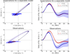Fig. 6. Top-left panel: left-hand side Ysep(θ) of Eq. (15) as a function of the right-hand side CsepXsep(θ) of Eq. (15) for a separable model. Bottom-left panel: left-hand side Yobs(θ) of Eq. (15) as a function of the right-hand side CsepXobs(θ) of Eq. (15) for the observations. Top right panel: left-hand side Ysep(θ) and right-hand side CsepXsep(θ) of Eq. (15) as a function of distance for a separable model. Bottom right panel: left-hand side Yobs(θ) and right-hand side CsepXobs(θ) of Eq. (15) as a function of distance for the observations. We show angular distances up to 30 Mm where the supergranular velocities are largest. Further away from the center of the supergranule, both X(θ) and Y(θ) go to zero. In all panels the errors are 3σ. In all panels, blue error bars and curves correspond to the right-hand side of Eq. (15) and red error bars and curves correspond to the left-hand side of Eq. (15).

The top-left panel of Fig. 6 shows that Eq. (15) is satisfied by the separable model and there is a clear proportionality relationship between X^sep(θ) and Y^sep(θ).

The bottom panels of Fig. 6 show that there is no coefficient C^obs such that Y^obs(θ) = C^obsX^obs(θ) within 3σ at all points for the observations. Close to the center of the supergranule (θR_⊙ ≤ 5 Mm), the condition defined by Eq. (15) holds within 3σ. Between θR_⊙ = 8 Mm and θR_⊙ = 16 Mm, the observations are 12σ_X away from satisfying Eq. (15). The signal at distances larger than 30 Mm is dominated by noise and oscillates around zero. The amplitude of these oscillations is of the same order of magnitude as the error estimates on the observations, and therefore we do not make any conclusions regarding this region.

To summarize, surface observations of an average supergranule are not consistent with separable models.

4.2. Influence of the horizontal scales of supergranules included in the average supergranule

The averaging process includes 10⁴ supergranules of different horizontal sizes. The nonseparability of the average supergranule does not necessarily imply that the flow fields of the individual supergranules are not separable. For example, a flow, defined as

$$\begin{array}{c}\hfill v_{\mathrm{r}}(r,\theta )=sin(2r)P_{\ell }(cos\theta )+sin(r)P_{2\ell }(cos\theta ),\end{array}$$(21)

is not separable for ℓ >  0.

During the identification of individual supergranules in LCT and Doppler travel-time maps (see Fig. 2), the supergranules were divided into four bins based on their size with the same number of supergranules in each bin.

Figure 7 shows the same quantities as in Fig. 6 for the four different bins. In all panels the errors are 3σ. The error estimates are twice as big as the error estimates for the full observations. This is expected from a data set cut in four equal pieces.

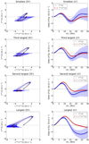Fig. 7. As in Fig. 6, with the same color scheme, for the averaging process performed on bins of supergranules categorized by area and strength. In all panels, the errors are 3σ. Average supergranules computed over a selected range of horizontal scales are still not compatible with separable models.

The area and strength of supergranules are correlated: weaker supergranules appear small independently of their actual size on divergence travel-time maps (as evidenced by Meunier et al. 2007). The largest supergranules on the travel-time maps are thus also the strongest, and the smallest ones are also the weakest.

If the average only contains the smallest and weakest supergranules, the observed velocity components are consistent with a separable model within three error bars (top panel of Fig. 7) because the signal-to-noise ratio is very small.

The larger and stronger the supergranules, the further away the observations get from separability. For the largest and strongest supergranules the observations are nine standard deviations away from separability.

The range of scales going into the averaging process cannot account for the incompatibility between separable models and the observations.

5. Conclusion

We confronted observations with the hypothesis that average supergranules are separable in terms of their vertical and horizontal structure. Separable models are not compatible with the observed surface flows.

Selecting the scales included in the average supergranule showed that the deviation from flow separability is more prominent for the largest spatial scales than it is for the smallest scales. The multiple horizontal scales of supergranules included in the average do not account for the incompatibility between observations and separability.

This result does not depend on the weighting functions involved in the computation of the surface velocity components, nor does it depend on the free parameters of separable models.

Nonseparable models are necessary to reproduce velocity observations for an average supergranule. Furthermore, the bottom-right panel of Fig. 6 imposes a new constraint on flow models used to represent supergranulation.

Any nonseparable flow model can be written as a sum of separable models. One possible example is an expansion of the horizontal variations on Legendre polynomials as was performed in Eq. (19) with a different r dependence at each ℓ.

Acknowledgments

R.F. is a member of the International Max Planck Research School for Solar System Science at the University of Göttingen. The HMI data used are courtesy of NASA/SDO and the HMI science team. The data were processed at the German Data Center for SDO (GDC-SDO), funded by the German Aerospace Center (DLR). The surface observations were treated and provided by Jan Langfellner. Aaron Birch, Robert Cameron and Laurent Gizon designed this research and contributed a lot of helpful comments. LG provided the equations in Sect. 3.2. RC suggested the specific approach used here to test separable models.

References

Appendix A: Error estimates

To determine the error on X(θ), we first approximate X(θ) at each point θ_n with

$$\begin{array}{c}\hfill X({\theta }_n)={\displaystyle \sum _{i=0}^n{v}_{\mathrm{r}}^{\mathrm{obs}}({\theta }_i)sin({\theta }_i)\mathrm{\Delta }\theta },\end{array}$$(A.1)

where Δθ is the step between two points in the horizontal direction. Here Δθ = 0.348 Mm. A property of the standard deviation on a set of random variables (x_i)_{1 ≤ i ≤ n} is that

$$\begin{array}{c}\hfill \sigma \left({\displaystyle \sum _{i=0}^n{x}_i}\right)\le {\displaystyle \sum _{i=0}^n\sigma (x_i)},\end{array}$$(A.2)

where σ is the standard deviation. We assume the worst case where σ_X is equal to the upper bound of Eq. (A.2)

$$\begin{array}{cc}\hfill {\sigma }_X({\theta }_n)& ={\displaystyle \sum _{i=0}^n\sigma (v_{\mathrm{r}}^{\mathrm{obs}}({\theta }_i)sin({\theta }_i)\mathrm{\Delta }\theta )}\hfill \\ \hfill & ={\displaystyle \sum _{i=0}^n}{\sigma }_{\mathrm{r}}({\theta }_i)sin({\theta }_i)\mathrm{\Delta }\theta \hfill \\ \hfill & \simeq {\displaystyle {\int }_0^{{\theta }_n}{\sigma }_{\mathrm{r}}({\theta }^{\prime })sin({\theta }^{\prime })}\mathrm{d}{\theta }^{\prime },\hfill \end{array}$$(A.3)

where, as discussed previously, σ_r(θ) is the error on the observed vertical velocity.

All Figures

	Fig. 1. Geometry of the problem. The black arrows show the unitary coordinate vectors. The center of the coordinate system coincides with the center of the Sun. The coordinate r is the radius (r = R⊙ at the photosphere shown in red) and θ is the heliocentric angular distance from the center of the supergranule. Hypothetical supergranular flows are shown in blue.
In the text

Fig. 2. Identification of supergranules (green crosses) in an example 8 h map of divergence-sensitive f-mode travel times computed at the equator, near disk center, using the method in Langfellner et al. (2015a). The x coordinate is in the east-west direction (positive towards west), the y coordinate is in the north-south direction (positive towards north). The gray-scale indicates the value of the divergence-sensitive travel times from which we derive the position of the supergranules. White indicates outflows, black inflows.

In the text

	Fig. 3. Assumed weighting function WLCT (see Eq. (5)) as a function of height with the parameters used in this paper.
In the text

	Fig. 4. Horizontal (top panel) and vertical (bottom panel) components of the velocity at the surface. The x coordinate is in the east-west direction (pointed westwards), the y coordinate is in the north-south direction (pointed northwards). The maps are centered at the center of the supergranule. Red indicates outflows (horizontal component) and upflows (vertical component).
In the text

	Fig. 5. Top panel: observed vertical velocity vr (blue curve) and horizontal velocity vθ (red curve) for an average supergranule as a function of the surface distance θR⊙ from the center of the supergranule. Bottom panel: error estimates on the LCT observations (red curve) and Doppler observations (blue curve).
In the text

Fig. 6. Top-left panel: left-hand side Ysep(θ) of Eq. (15) as a function of the right-hand side CsepXsep(θ) of Eq. (15) for a separable model. Bottom-left panel: left-hand side Yobs(θ) of Eq. (15) as a function of the right-hand side CsepXobs(θ) of Eq. (15) for the observations. Top right panel: left-hand side Ysep(θ) and right-hand side CsepXsep(θ) of Eq. (15) as a function of distance for a separable model. Bottom right panel: left-hand side Yobs(θ) and right-hand side CsepXobs(θ) of Eq. (15) as a function of distance for the observations. We show angular distances up to 30 Mm where the supergranular velocities are largest. Further away from the center of the supergranule, both X(θ) and Y(θ) go to zero. In all panels the errors are 3σ. In all panels, blue error bars and curves correspond to the right-hand side of Eq. (15) and red error bars and curves correspond to the left-hand side of Eq. (15).

In the text

	Fig. 7. As in Fig. 6, with the same color scheme, for the averaging process performed on bins of supergranules categorized by area and strength. In all panels, the errors are 3σ. Average supergranules computed over a selected range of horizontal scales are still not compatible with separable models.
In the text

References

- Abramowitz, M., & Stegun, I. 1965, Handbook of Mathematical Functions: With Formulas, Graphs, and Mathematical Tables, Applied Mathematics Series (Dover Publications) [Google Scholar]
- Bello González, N., Yelles Chaouche, L., Okunev, O., & Kneer, F. 2009, A&A, 494, 1091 [NASA ADS] [CrossRef] [EDP Sciences] [Google Scholar]
- Bhattacharya, J., Hanasoge, S. M., Birch, A. C., & Gizon, L. 2017, A&A, 607, A129 [NASA ADS] [CrossRef] [EDP Sciences] [Google Scholar]
- Christensen-Dalsgaard, J., Dappen, W., Ajukov, S. V., et al. 1996, Science, 272, 1286 [CrossRef] [Google Scholar]
- DeGrave, K., & Jackiewicz, J. 2015, Sol. Phys., 290, 1547 [NASA ADS] [CrossRef] [Google Scholar]
- Dombroski, D. E., Birch, A. C., Braun, D. C., & Hanasoge, S. M. 2013, Sol. Phys., 282, 361 [NASA ADS] [CrossRef] [Google Scholar]
- Duvall, Jr., T. L., & Birch, A. C. 2010, AJ, 725, L47 [Google Scholar]
- Duvall, Jr., T. L., & Gizon, L. 2000, Sol. Phys., 192, 177 [NASA ADS] [CrossRef] [Google Scholar]
- Duvall, T. L., & Hanasoge, S. M. 2013, Sol. Phys., 287, 71 [NASA ADS] [CrossRef] [Google Scholar]
- Duvall, T. L., D’Silva, S., Jefferies, S. M., Harvey, J. W., & Schou, J. 1996, Nature, 379, 235 [NASA ADS] [CrossRef] [Google Scholar]
- Fleck, B., Couvidat, S., & Straus, T. 2011, Sol. Phys., 271, 27 [NASA ADS] [CrossRef] [Google Scholar]
- Gizon, L. 2006, SOHO-17. 10 Years of SOHO and Beyond, ESA Spec. Pub., 617, 5.1 [Google Scholar]
- Hart, A. B. 1954, MNRAS, 114, 17 [NASA ADS] [CrossRef] [Google Scholar]
- Hathaway, D. H., Beck, J. G., Bogart, R. S., et al. 2000, Sol. Phys., 193, 299 [NASA ADS] [CrossRef] [Google Scholar]
- Hathaway, D. H., Beck, J. G., Han, S., & Raymond, J. 2002, Sol. Phys., 205, 25 [NASA ADS] [CrossRef] [Google Scholar]
- Hirzberger, J., Gizon, L., Solanki, S. K., & Duvall, T. L. 2008, Sol. Phys., 251, 417 [NASA ADS] [CrossRef] [Google Scholar]
- Langfellner, J., Gizon, L., & Birch, A. C. 2015a, A&A, 581, A67 [NASA ADS] [CrossRef] [EDP Sciences] [Google Scholar]
- Langfellner, J., Gizon, L., & Birch, A. C. 2015b, A&A, 579, L7 [NASA ADS] [CrossRef] [EDP Sciences] [Google Scholar]
- Leighton, R. B., Noyes, R. W., & Simon, G. W. 1962, AJ, 135, 474 [CrossRef] [Google Scholar]
- Meunier, N., Tkaczuk, R., Roudier, T., & Rieutord, M. 2007, A&A, 461, 1141 [NASA ADS] [CrossRef] [EDP Sciences] [Google Scholar]
- November, L. J., & Simon, G. W. 1988, AJ, 333, 427 [NASA ADS] [CrossRef] [Google Scholar]
- Pesnell, W. D., Thompson, B. J., & Chamberlin, P. C. 2012, Sol. Phys., 275, 3 [NASA ADS] [CrossRef] [Google Scholar]
- Rieutord, M., & Rincon, F. 2010, Sol. Phys., 7, 2 [Google Scholar]
- Rieutord, M., Roudier, T., Ludwig, H.-G., Nordlund, Å., & Stein, R. 2001, A&A, 377, L14 [NASA ADS] [CrossRef] [EDP Sciences] [Google Scholar]
- Rieutord, M., Roudier, T., Rincon, F., et al. 2010, A&A, 512, A4 [NASA ADS] [CrossRef] [EDP Sciences] [Google Scholar]
- Ritzwoller, M. H., & Lavely, E. M. 1991, AJ, 369, 557 [Google Scholar]
- Schou, J., Scherrer, P. H., Bush, R. I., et al. 2012, Sol. Phys., 275, 229 [Google Scholar]
- Simon, G. W., & Leighton, R. B. 1964, AJ, 140, 1120 [Google Scholar]
- Snodgrass, H. B. 1984, Sol. Phys., 94, 13 [NASA ADS] [CrossRef] [Google Scholar]