| Issue |
A&A
Volume 622, February 2019
|
|
|---|---|---|
| Article Number | A153 | |
| Number of page(s) | 13 | |
| Section | Planets and planetary systems | |
| DOI | https://doi.org/10.1051/0004-6361/201834569 | |
| Published online | 13 February 2019 | |
The CARMENES search for exoplanets around M dwarfs
The enigmatic planetary system GJ 4276: one eccentric planet or two planets in a 2:1 resonance?★
1
Hamburger Sternwarte,
Gojenbergsweg 112,
21029 Hamburg,
Germany
e-mail: This email address is being protected from spambots. You need JavaScript enabled to view it.
2
Universität Göttingen, Institut für Astrophysik,
Friedrich-Hund-Platz 1,
37077 Göttingen,
Germany
3
Instituto de Astrofísica de Andalucía (IAA-CSIC),
Glorieta de la Astronomía s/n,
18008 Granada,
Spain
4
School of Physics and Astronomy, Queen Mary, University of London,
327 Mile End Road,
London
E1 4NS,
UK
5
Institut de Ciències de l’Espai (ICE, CSIC),
Campus UAB, C/ de Can Magrans s/n,
08193 Cerdanyola del Vallès,
Spain
6
Institut d’Estudis Espacials de Catalunya (IEEC),
C/ Gran Capità 2-4,
08034 Barcelona,
Spain
7
Landessternwarte, Zentrum für Astronomie der Universtät Heidelberg,
Königstuhl 12,
69117 Heidelberg,
Germany
8
Centro de Astrobiología (CSIC-INTA),
ESAC, Camino Bajo del Castillo s/n,
28692 Villanueva de la Cañada,
Madrid,
Spain
9
Centro Astronómico Hispano-Alemán (CSIC-MPG), Observatorio Astronómico de Calar Alto,
Sierra de los Filabres,
04550 Gérgal,
Almería,
Spain
10
Instituto de Astrofísica de Canarias,
Vía Láctea s/n,
38205 La Laguna,
Tenerife,
Spain
11
Departamento de Astrofísica, Universidad de La Laguna,
38206 La Laguna,
Tenerife,
Spain
12
Thüringer Landessternwarte Tautenburg,
Sternwarte 5,
07778 Tautenburg,
Germany
13
Max-Planck-Institut für Astronomie,
Königstuhl 17,
69117 Heidelberg,
Germany
14
Departamento de Astrofísica y Ciencias de la Atmósfera, Facultad de Ciencias Físicas, Universidad Complutense de Madrid,
28040 Madrid,
Spain
Received:
3
November
2018
Accepted:
13
December
2018
Abstract
We report the detection of a Neptune-mass exoplanet around the M4.0 dwarf GJ 4276 (G 232-070) based on radial velocity (RV) observations obtained with the CARMENES spectrograph. The RV variations of GJ 4276 are best explained by the presence of a planetary companion that has a minimum mass of mb sin i ≈ 16 M⊕ on a Pb = 13.35 day orbit. The analysis of the activity indicators and spectral diagnostics exclude stellar induced RV perturbations and prove the planetary interpretation of the RV signal. We show that a circular single-planet solution can be excluded by means of a likelihood ratio test. Instead, we find that the RV variations can be explained either by an eccentric orbit or interpreted as a pair of planets on circular orbits near a period ratio of 2:1. Although the eccentric single-planet solution is slightly preferred, our statistical analysis indicates that none of these two scenarios can be rejected with high confidence using the RV time series obtained so far. Based on the eccentric interpretation, we find that GJ 4276 b is the most eccentric (eb = 0.37) exoplanet around an M dwarf with such a short orbital period known today.
Key words: planetary systems / stars: individual: GJ 4276 / stars: low-mass / methods: data analysis / methods: observational / techniques: radial velocities
Photometric measurements and Table C.1 are available at the CDS via anonymous ftp to cdsarc.u-strasbg.fr (130.79.128.5) or via http://cdsarc.u-strasbg.fr/viz-bin/qcat?J/A+A/622/A153
© ESO 2019
1. Introduction
M dwarfs constitute roughly 75% of the stellar population in the solar neighborhood (Henry et al. 2006). Compared to solar-like stars, they are smaller in mass, radius, and luminosity. These properties shift the focus of ongoing and future transit and radial velocity (RV) surveys toward M dwarfs for many reasons. Since the semi-amplitude of the reflex motion scales with stellar mass as  (e.g., Cumming et al. 1999) and the transit depth with the stellar radius as
  (e.g., Seager & Mallén-Ornelas 2003), they are most promising targets for exoplanet searches and, in particular, for finding Earth-like rocky planets. Of special interest are planets located in the habitable zone, in which water can exist on the planetary surface in a liquid phase. Due to the intrinsic faintness of M dwarfs, the distance of the habitable zone is much smaller for those stars. This leads to shorter orbital periods and larger transit probabilities. Early M dwarfs show a high planet occurrence rate of 2.5 ± 0.2 planets with 1−4 Earth radii and orbital periods shorter than 200 days per star (Dressing & Charbonneau 2015), implying that these objects are numerous planet hosts in the Milky Way.
The search for low-mass planets around a sample of about 300 M dwarfs (Reiners et al. 2018a) is the main scientific objective of the RV survey conducted by the CARMENES consortium (Quirrenbach et al. 2018). The CARMENES instrument has already proved its ability to reach an RV accuracy of ~1 m s−1 and has enabled the discovery and characterization of several planetary systems (Trifonov et al. 2018; Reiners et al. 2018b; Sarkis et al. 2018; Kaminski et al. 2018; Luque et al. 2018; Ribas et al. 2018).
In this paper, we report the detection of a Neptune-mass object orbiting GJ 4276. In Sect. 2, we present the stellar characteristics of GJ 4276. The photometric data sets and the determination of the rotation period are described in Sect. 3. We performed a detailed analysis of the RV measurements and the stellar activity, and fit Keplerian models to the RV data, as described in Sect. 4. Finally, we summarize and discuss our findings in Sect. 5.
2. Host star properties
We summarize the main characteristics of our star in Table 1. GJ 4276 (G 232-070, Karm J22252 + 594) is an M4.0 dwarf (Reid et al. 1995; Lépine et al. 2013) at a distance of 21.35 ± 0.02 pc (Gaia Collaboration 2018). Together with the parallax, we used the proper motion in right ascension and declination to calculate the secular acceleration ( m s−1 yr−1). The UV W Galactic space velocities imply that GJ 4276 belongs to the thin-disk stellar population (Cortés-Contreras 2016).
The basic photospheric parameters Teff, log g, and [Fe/H] were measured as in Passegger et al. (2018), who fit the latest version of the PHOENIX-ACES models (Husser et al. 2013) to CARMENES spectra. We computed the luminosity from the Gaia DR2 parallax and multiwavelength photometry from B to W4 as described in Kaminski et al. (2018) and Luque et al. (2018). Based on our Teff and L determinations, we computed the stellar radius R by means of the Stefan-Boltzmann law, and finally derived the stellar mass M using a linear mass-radius relation. The details of the luminosity, radius, and mass determinations of the CARMENES targets will be presented by Cifuentes et al. (in prep.) and Schweitzer et al. (in prep.).
The star GJ 4276 is not a ROSAT All-Sky Survey (RASS) source and we estimated an upper limit for the X-ray luminosity of LX ≈ 8 × 1027 erg s−1 using the typical RASS detection limit of fX ≈ 2 × 10⁻¹³ erg cm−2 s−1 (Schmitt et al. 1995) and, from it, an upper limit of LX ∕Lbol < 10−4. According to Reiners et al. (2018a), GJ 4276 is not an Hα emitter and has an 2 km s−1 upper limit on the projected rotational velocity v sin i.
3. Photometry
To search for photometric modulation caused by rotating surface inhomogeneities such as dark spots and bright plages, we used archival time-series photometry from the MEarth-North project (Berta et al. 2012) and the “All-Sky Automated Survey for Supernovae” (ASAS-SN; Shappee et al. 2014). In addition, we obtained custom V band photometry with the T150 telescope located at the Sierra Nevada Observatory (SNO) in Spain and with two 40 cm telescopes of the Las Cumbres Observatory (LCO) located at the Haleakala Observatory on Hawai’i and the Teide Observatory on the Canary Islands.
The MEarth-North telescope array is located at the Fred Lawrence Whipple Observatory, Arizona, and consists of eight 40 cm robotic telescopes. Each is equipped with a 2048 × 2048 CCD with a pixel scale of 0.76″ and a custom 715 nm longpass filter. While the main objective of the MEarth project is the search for low-mass rocky exoplanets around M dwarfs in the habitable zone with the transit method, ASAS-SN is dedicatedto the discovery of nearby supernovae by monitoring the entire visible sky down to ~17 mag in the V band. It comprises five units with a total of 20 telescopes situated in Chile, Hawai’i, South Africa, and Texas. Each of the 14 cm telephoto lenses has a 2k × 2k CCD with a field of view of 4.5 × 4.5 deg and a pixel scale of 7.8″. The T150 telescope at the SNO is a 150 cm Ritchie-Chétien telescope. It is equipped with a 2k × 2k VersArray CCD camera with a field of view of 7.9 × 7.9 arcmin (Rodríguez et al. 2010). The LCO telescopes are equipped with a 3k × 2k SBIG CCD camera with a pixel scale of 0.571″ providing a field of view of 29.2 × 19.5 arcmin.
The photometric measurements used in this study cover a time span of four years of MEarth data (October 2011–November 2015), three years of ASAS-SN data (December 2014–December 2017), four months of SNO data (May–September 2018), and three months of LCO data (June–September 2018). Exposure times of ten minutes for MEarth and ASAS-SN, 50 seconds for SNO, and 150 seconds for LCO result in median uncertainties of  mmag,
mmag,  mmag,
mmag,  mmag, and
  mmag.
mmag.
To identify potentially spot induced periodic variability, we applied the generalized Lomb-Scargle (GLS) periodogram (Zechmeister & Kürster 2009) to the MEarth, ASAS-SN, and SNO data sets of GJ 4276. The periodograms show evidence for periodicity at  d,
d,  d, and
  d. To estimate the uncertainties of our period determination, we fit a Gaussian profile to the peak with the largest power and computed its full-width-half-maximum (FWHM).
We present the light curve, the periodogram, and the phase folded light curve derived from the SNO data in Fig. 1. The light curves and periodograms of the MEarth and ASAS-SN data sets are shown in Fig. A.1. Visual inspection of the SNO light curve (top panel of Fig. 1) shows a clear variability pattern, which remained rather stable during the observation run. The pattern is well resolved and consists of two bumps with alternating amplitude, which we interpret as the photometric manifestation of two starspots located on opposing hemispheres. Therefore, we conclude that the GLS peak at 32.3 days is the semi-period of the stellar rotation period of ≈64.6 d, which also resolves the apparent conflict with the MEarth and ASAS-SN data. The phase-folded light curves of the latter show a less pronounced signal, which may be related to the longer span covered. We find consistent results with the LCO data.
The rotation period obtained here is consistent with the findings of Díez Alonso et al. (2019), who reported a value of 64.6 ± 2.1 d with a FAP level of <10−4% for GJ 4276 based on their analysis of the ASAS-SN light curve alone. Also, a rotation period of roughly 64 days is consistent with the low activity level observed in GJ 4276 and the absence of Hα emission. Based on gyrochronological models by Barnes (2007), we calculated an age of 6.9 ± 1.1 Gyr using the intrinsic B−V color and the derived rotation period as input parameters.
Stellar parameters of GJ 4276.
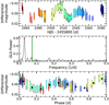 |
Fig. 1. Rotation period analysis using SNO photometric data. Top panel: V band light curve. The color of the datapoints indicates the observation epoch. Middle panel: GLS periodogram. The vertical green line represents the orbital period of the planet at 13.35 days and the red dot the peak with the highest power at 32.3 days. Bottom panel: phased light curve using twice the period derived from the GLS. The black squares indicate the mean magnitude in ten equidistant bins in phase. |
4. Spectroscopy
We gathered exactly 100 CARMENES RV measurements of GJ 4276 over a time span of 774 days. The observations were carried out as part of the CARMENES GTO survey (Reiners et al. 2018a) between July 2016 and August 2018 with the CARMENES echelle spectrograph (Quirrenbach et al. 2018), mounted on the 3.5 m telescope of the Calar Alto Observatory in Spain. CARMENES consists of a pair of high resolution spectrographs, which cover the optical wavelength range from 5200 Å to 9600 Å with a resolution power of R = 94 600, and the near-infrared range from 9600 Å to 17 100 Å with R = 80 400. Both channels areenclosed in temperature- and pressure-stabilized vacuum vessels to reduce instrumental drifts and to provide a RV precision on a m s−1 level.
The CARMENES survey observation strategy aims at reaching a signal-to-noise ratio of 150 in the J band. The typical exposure time of our spectra of GJ 4276 is 1800 s. The raw frames were extracted using the CARACAL reduction pipeline (Caballero et al. 2016), which is based on flat-relative optimal extraction (Zechmeister et al. 2014). The wavelength calibration is based on three hollow cathode lamps (U-Ne, U-Ar, and Th-Ne) combined with a Fabry-Pérot etalon (Bauer et al. 2015; Schäfer et al. 2018). The reference frames were taken at the beginning of each observing night. In addition, Fabry-Pérot etalon spectra were taken simultaneously with the target to track and correct the nightly instrument drift.
To precisely measure the Doppler shifts on a m s−1 level, we used the SERVAL1 code (Zechmeister et al. 2018), which constructs a high signal-to-noise template spectrum by coadding all spectra of GJ 4276 after correcting for barycentric motion (Wright & Eastman 2014) and secular acceleration (Zechmeister et al. 2009). To consider systematic instrumental effects, we further corrected the RVs for nightly zero-point variations using RV measurements of stars with low RV variability observed in the same night; we refer to Trifonov et al. (2018) for a detailed description.
In this study, we employed RVs only from the VIS channel, which have an internal median uncertainty of 1.7 m s−1. We present the RV measurements used in this paper in Fig. 2 and list them along with their formal uncertainties in Table C.1.
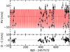 |
Fig. 2. Top panel: radial velocity measurements of GJ 4276 obtained with CARMENES as a function of barycentric Julian Date. The best-fit eccentric single-planet Keplerian model is overplotted in red (see Sect. 4.2). Bottom panel: O − C residuals. |
4.1. Periodogram analysis
To study the RV variability of GJ 4276, we applied the GLS periodogram to the measurements obtained with CARMENES. The resulting periodogram is shown in Fig. 3. Following Eq. (24) from Zechmeister & Kürster (2009), we computed the false alarm probabilities (FAPs) to evaluate the significance of the peaks in the power spectra.
The largest power excess with a FAP well below 0.1% appears at a frequency of f = 0.07493 d−1 (13.347 days, Fig. 3a). To check the persistence of this signal, we divided the entire data set into three RV subsamples and separately analyzed their periodograms. In all cases we find similar peaks, corresponding to frequencies of f1 = 0.07480 d−1 (13.370 days), f2 = 0.07438 d−1 (13.444 days), and f3 = 0.07581 d−1 (13.192 days), indicating that the signal is, indeed, persistent. Furthermore, a power peak of the first harmonic of the dominant signal at f = 0.14986 d−1 (6.673 days) is visible in the periodogram.
We identify further strong signals with FAPs < 0.1% at frequencies of 0.92784 d−1 and 1.07766 d−1 with powers of 0.51 and 0.58, respectively (outside the frequency range shown in Fig. 3 for the sake of clarity). Both peaks are plausible one-day aliases of the primary period (~ 1.000 ± 0.075 d−1) which disappear after we subtract the best-fit eccentric single-planet Keplerian model (see Sect. 4.2.2) from the RV measurements.
To ensure that the RV variation is not caused by stellar activity, we made use of several spectral diagnostics provided by SERVAL, viz., chromospheric indices, the differential line width, the chromatic index, and the cross-correlation function. The chromatic index (CRX), as introduced by Zechmeister et al. (2018), describes the color-dependence of the RV signal, which must vanish for a planetary signal but not for a spot-induced signal. Rotating spots induce periodic line profile variations, which were scrutinized using the differential line width (dLW) indicator. We also analyzed the cross-correlation function (CCF) of each spectrum. Specifically, we checked for periodic modulation of the FWHM, contrast, and bisector span as described in Reiners et al. (2018b). Any such detection would, again, be a red flag indicating activity-induced modulation. Finally, the Hα and Ca II IRT line indices were analyzed, which directly trace chromospheric activity.
We present GLS periodograms of all these spectral diagnostic time series in Fig. 3. Beside the periodogram of the dLW and Ca II IRT b line indices at 8542 Å, none of the investigated indicators exhibit significant peaks above the 10% FAP level. The periodogram of the dLW shows a marginally significant power peak at the first harmonic of the stellar rotation period around 32 days, which is most likely caused by rotational modulation of active regions. In addition, the dLW shows two peaks at 54 and 161 days with formal FAP levels above 10% and 0.1%, respectively. Also, some long-term periodic pattern can be seen in the periodogram of the Ca II IRT b line index but no peaks were found in the periodograms of the Ca II IRT a and c line indices at 8498 Å and 8662 Å at similar frequencies. Importantly, however, the RV signal at 13.347 days correlates neither with the spurious signals produced by the dLWand the Ca II IRT b line indices nor with any signal produced by other spectral activity indicators. Thus, we are confident that this persistent signal is not related to activity, but is most probably of planetary origin.
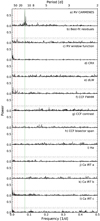 |
Fig. 3. GLS periodograms of GJ 4276. Panel a: periodogram of the CARMENES RVs. The horizontal lines (dotted, dash-dotted, dashed) indicate FAP levels of 10%, 1%, and 0.1%. The vertical green line marks the orbital period with the highest power at 13.347 d. The left red dashed line at Prot = 64.3 d (frot = 0.0156 d−1) shows the weighted mean of the photometrically derived stellar rotation period and the right red dashed line its first harmonic (2frot = 0.0311 d−1). Panel b: periodogram of the residuals after removing the best-fit single-planet Keplerian with eccentricity (see Sect. 4.2.2) signal; panel c: window function of the RV data. Panels d–h: periodograms of the chromatic RV index (CRX), differential line width (dLW), as well as FWHM, contrast, and bisector span from the CCF analysis. Panels i–l: periodograms of the chromospheric line indices of Hα and Ca II IRT. |
4.2. Orbital solutions
Having established the planetary origin of the RV signal, we now determine the orbital elements of the planet. To that end, we implemented a Keplerian RV curve model and carry out parameter optimization using a Nelder-Mead simplex algorithm (Nelder & Mead 1965). Following the approach of Baluev (2009), our model incorporates an RV jitter variance term to account for additional stochastic scatter; the jitter parameter is fit simultaneously during the parameter optimization.
In the following, we juxtapose three Keplerian models and their performance in describing the observations, in particular, asingle planet with a circular orbit, a single planet with an eccentric orbit, and two planets with circular orbits with a period ratio of 2:1. In addition to the periodic planetary signal, we allow for an RV offset to account for entire system’s velocity. In a first run, we further fit a linear time evolution parameter to derive potential systematic acceleration and gauged with a likelihood ratio test whether the improvement is sufficient to include a slope. Although this additional fitting parameter resulted in a higher likelihood, we find that the improvement is non-significant.
The entire set of the derived best-fit Keplerian orbital elements is displayed in Table 2. The 1σ uncertainties of the orbital parameters are estimated from the posterior distributions using the Markov Chain Monte Carlo sampler emcee (Foreman-Mackey et al. 2013) along with our Keplerian models (Figs. B.1–B.3). For the fit parameters we assumed uniform priors, except for the stellar mass, for which we imposed a Gaussian prior with mean and variance equal to 0.406 ± 0.030 M⊙ based on the mass determination of GJ 4276 (Sect. 2).
Best-fit orbital parameters for the GJ 4276 system.
4.2.1. Single planet on circular orbit
In the first model, we fit the RV measurements with a single planet on a circular orbit. We left the semi-amplitude Kb, the orbital period Pb, the RV jitter σjitter, as well as the RV offset γ as free parameters. The eccentricity remained fixed to eb = 0. Further, we also fixed the argument of the periapsis to ωb = 90 deg and fit the time of the periastron passage τb.
This model converges on a period of Pb = 13.348 days, matching the frequency of the power peak found in the periodogram. Following a Keplerian interpretation of the RV variations, GJ 4276 b is a Neptune-like planet with a minimum mass of mb sin i = 16.11 M⊕. Orbiting at a distance of 0.082 au from its host star, it is placed closer than the inner edge of the conservative and optimistic habitable zones, which range from 0.146 to 0.284 au and 0.115 to 0.299 au, respectively (Kopparapu et al. 2013, 2014). The solution further yields a semi-amplitude of Kb = 7.93 m s−1 and a jitter term of σjitter = 2.83 m s−1. With respect to the model, the data yield a root mean square (rms) value of σO-C = 3.29 m s−1.
4.2.2. Single planet with eccentric orbit
In addition to the parameters from the circular solution, we here let the eccentricity e and the argument of the periapsis ωb vary freely. While the best-fit minimum mass, the orbital period, semi-amplitude, and semi-major axis are comparable to that of the single-planet circular solution (mb sin i = 16.57 M⊕, Pb = 13.352 d, Kb = 8.79 m s−1, ab = 0.082 au), the jitter term of σjitter = 1.74 m s−1 found here is 1.09 m s−1 smaller than that previously obtained. The introduction of the eccentricity eb = 0.37 significantly improves the fit and results in an rms of σO-C = 2.46 m s−1. We show the phased RV data and the best-fit Keplerian one-planet solution in Fig. 4.
4.2.3. Two planets on circular orbits with period ratio of 2:1
The single-planet model with an eccentric orbit results in a remarkably eccentric orbit with e = 0.37. Since the Doppler signal of a two-planet system on circular orbits near a 2:1 mean motion resonance can be misinterpreted as an eccentric single-planet (Anglada-Escudé et al. 2010; Wittenmyer et al. 2013; Kürster et al. 2015; Boisvert et al. 2018), we further tried to fit a two-planet model with circular orbits and fixed period ratio of 2:1, i.e., Pb = 2Pc. In the modeling, we leave Kb, Kc, Pb, τb, τc, γ, and σjitter free to vary (whereas ωb = ωc = 90 deg).
Based on this double Keplerian model, we obtained orbital parameters for GJ 4276 b: Kb = 7.67 m s−1, Pb = 13.350 days, and for GJ 4276 c: Kc = 2.73 m s−1, Pc = 6.675 days, which translates into minimum planetary masses of mb sin i = 15.58 M⊕ and mc sin i = 4.40 M⊕ and semi-major axes of ab = 0.082 au and ac = 0.051 au.
4.3. Likelihood analysis
To compare the fit qualities between the eccentric single-planet model and the two-planet model compared to the circular single-planet model, we carried out likelihood ratio tests (e.g., Wilks 1938; Protassov et al. 2002). In our circular single-planet model we have five free parameters, while there are seven in both the single-planet model with elliptical orbit and our two-planet model. The test statistic is  . According to Wilk’s theorem (Wilks 1938), the probability distribution of the test statistic can be approximated by a χ2 distribution with df degrees of freedom for large data samples. However, as discussed by Protassov et al. (2002), Baluev (2009), and Czesla & Schmitt (2010), the formal criteria for this approximation are not fulfilled in the current case. While the models are nested as required, the circular single-planet model is only obtained from our elliptical or two-planet models by choosing parameters at the edge of the parameter space such as zero eccentricity.
Therefore, we verified that the probability distribution of the test statistic can, indeed, be approximated by a χ2 distribution with two degrees of freedom:
 (1)
(1)
Based on the best-fit circular single-planet solution, we generated 1000 synthetic data sets with random normally distributed errors that include the measurement error and the maximum-likelihood estimate of the stellar jitter so that  . We fit these mock data sets using the circular single-planet model, as well as the eccentric single-planet and two-planet models. Based on the maxima of the respective likelihood functions, we calculated the test statistic
  . As an example, we show the simulated distribution of the likelihood ratio test statistic, as well as the χ2 distribution, for the comparison of the circular single-planet model and the eccentric single-planet model in Fig. 5. Based on our simulations, we conclude that the χ2 distribution yields an acceptable approximation to the distribution of the test statistic in our case.
To assess the fit quality of the eccentric single-planet model compared to the circular single-planet model, we computed the ratio of the best-fit likelihoods for the circular model  and eccentric model
  and found a value of
  . The probability to obtain such an improvement by chance if the true orbit were circular is only 1.4 × 10⁻¹³. The comparison between the circular single-planet scenario and the two-planet model results in a likelihood ratio of
  , where
  is the best-fit likelihood of the circular two-planet model. Again, we find a probability of only 1.4 × 10⁻¹¹ that such an improvement in fit quality can be achieved by chance. We therefore conclude that the circular single-planet solution can be rejected with high confidence.
To study whether the eccentric single-planet model or the circular two-planet model is statistically preferred, we carried out another simulation. In particular, we generated 1000 artificial data sets by adding normally distributed random noise to the maximum-likelihood eccentric single-planet model on the one hand and the two-planet model on the other hand. To determine what differences in likelihood can be expected, we fit all of these artificial RV curves using both the eccentric single-planet and the two-planet model and calculated the likelihood ratios  and
and  , respectively. In Fig. 6 we show the resulting histograms of the likelihood ratios. We find a median value of − 5.02 assuming that the eccentric model is true and − 3.54 for the two-planet case. In addition, we indicate the measured likelihood ratio of
  . Based on the higher likelihood achieved in the fit, we find a slight preference for the eccentric single-planet solution. However, our findings show that the measured difference in likelihood does not allow to reject one or the other solution with reasonable confidence.
One possible strategy to discriminate between the two degenerated models is to increase the number of RV measurements, as suggested by Anglada-Escudé et al. (2010), Kürster et al. (2015), and Boisvert et al. (2018). Ideally, the observations should be carried out at phases of maximal differences between the models. In the case of GJ 4276 b, we find a maximal difference of 2.10 m s−1, which lies above the internal median error of 1.7 m s−1. However, even for a quiet star like GJ 4276, we found an activity-induced RV jitter level in the range of 1.5–3 m s−1 limiting the achievable RV accuracy. To provide a rough estimate on the amount of additional RV observations that are necessary to distinguish between the two solutions, we generated synthetic RV measurements based on the best-fit eccentric model and fit them with the eccentric and the two-planet Keplerian model. Our results imply that ~100 additional measurements randomly distributed in phase would be sufficient to push the likelihood ratio to  .
.
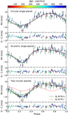 |
Fig. 4. Phase-folded radial velocity measurements of GJ 4276, together with the best-fit Keplerian model (black line) overplotted. In the bottom of each panel we show the O − C residuals. Top panel: circular single-planet Keplerian model. Middle panel: eccentric single-planet Keplerian model. Bottom panel: two-planet Keplerian model on circular orbits with a period ratio of 2:1. In addition, we show the best-fit Keplerian model of GJ 4276 b (green dashed line) and GJ 4276 c (red dotted line). |
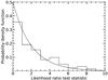 |
Fig. 5. Empirical distribution of the |

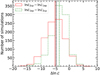 |
Fig. 6. Histograms of the likelihood ratio using simulated data sets based on the best-fit eccentric single-planet model (solid red) and the circular two-planet model (dashed green). The vertical solid red line and the dashed green line represent the median values of the histograms. The black dotted vertical line represents the measured likelihood ratio
|

4.4. Orbital evolution of the eccentric single-planet solution
We employed an estimate of the tidal circularization timescale for the eccentric one-planet solution in order to assess its plausibility compared to the two-planet solution. Following Jackson et al. (2008), we solved the coupled differential equation for the evolution of the semi major axis and eccentricity due to tidal interaction. The two parameters determining this evolution are the modified tidal dissipation values Q. Here we adopted Q⋆ = 105 for the star. For the planet we used Qp = 100 for a possible rocky planet and Qp = 105 for a Neptune-like planet. Due to the significantly higher dissipation, a rocky planet’s orbit would completely circularize within 108 yr, while a Neptune-like planet would maintain a high eccentricity over more than 10 Gyr. The unknown planetary interior therefore does not allow to provide an additional constraint to distinguish between the two configurations.
4.5. Search for additional planetary companions
To check whether the RV data yield evidence for additional planets, we removed the best-fit single-planet eccentric model and the circular two-planet model from the RV data and investigated the GLS periodograms of the RV residuals. Both periodograms show power excess at 32 days on a 10% FAP level, reflecting half of the stellar rotation period (see Fig. 3b). In addition to that, the periodograms of the RV residuals did not reveal any further significant power peaks attributable to planetary companions.
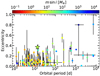 |
Fig. 7. Eccentricity plotted against orbital period of known exoplanets around M dwarfs (dots). The colors indicate the minimum mass and the star marks the position of GJ 4276 b with the eccentric single-planet solution. |
5. Summary and discussion
In this study, we analyzed 100 RV measurements of the M4.0V star GJ 4276, taken with the visible channel of the high-resolution CARMENES echelle spectrograph. The rotation period of 64 days determined from long-term photometry (MEarth, ASAS-SN) and the photometric campaign carried out during the present work (SNO, LCO), together with the lack of Hα emission, implies that GJ 4276 is a weakly active and slowly rotating star. The examination of the spectral diagnostics and the activity indicators revealed no link between stellar activity and the supposed planetary signal supporting the fact that the RV variation at this period arises from Keplerian motion of a planetary companion.
The orbital analysis is based on three distinct models: a circular single Keplerian, an eccentric single Keplerian, and two circular Keplerians in a likely 2:1 mean motion resonance. To compare the fit quality of the circular single-planet model with that of the more complex models, we carried out a likelihood ratio test. Both, the eccentric single-planet, as well as the circular two-planet solution, provide a significantly better solution than the circular single-planet solution, which we therefore rejected as a plausible explanation for the data. The eccentric single-planet model and the two-planet model are described by the same number of free parameters. As a matter of fact, the eccentric single planet model yields a higher likelihood and also a smaller jitter term on the grounds of which it might be preferred. To further quantify this statement, we generated synthetic data sets based on the eccentric and the two-planet solution, and inspected the likelihood ratio distributions. Our investigations show that none of the models can be rejected on statistical grounds. As both models are also physically plausible, we discuss their implications below.
Based on the eccentric model, GJ 4276 b has a minimum mass of ~16.6 M⊕, an orbital period of 13.4 days, and is located closer than the inner edge of the habitable zone at 0.08 au. At this orbital distance thetidal circularization timescale for a gaseous planet is more than 10 Gyr, which is consistent with an eccentric orbit. Analyzing the periodogram of the residual RVs, we find no immediate evidence for further planetary companions around GJ 4276. We shown in Fig. 7 the eccentricity of the known exoplanets around M dwarfs as a function of orbital period. There are 13 planetary systems with published eccentricities of e ≥ 0.3. With a relatively high eccentricity of 0.37 ± 0.03, GJ 4276 b would be among the most eccentric exoplanets around M dwarfs known to date and comparable with the recently published exoplanet GJ 96 b with 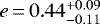 (Hobson et al. 2018). However, while both planets have similar masses, they differ significantly in the orbital period (
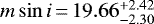 M⊕ and
 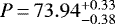 d for GJ 96 b).
A 2:1 mean motion resonance is found in many planetary systems such as HD 82943, HD 128311, HD 73526, HD 90043, and HD 27894 (Mayor et al. 2004; Vogt et al. 2005; Tinney et al. 2006; Johnson et al. 2011; Trifonov et al. 2017). So far, two systems with M dwarf host stars and planets near the 2:1 resonance are known, viz., GJ 876 (Marcy et al. 2001; Rivera et al. 2010) and TRAPPIST-1 (Gillon et al. 2017). Both of these systems harbor more than two known planets with orbital periods in a 4:2:1 resonance chain for GJ 876 and 8:5:3:2:1 for TRAPPIST-1. Given these examples, we consider a resonant two-planet system also a plausible model for GJ 4276. While we here focus on a strict 2:1 period ratio, we note that a slightly larger period ratio around 2.2 is often realized (Steffen & Hwang 2015). Also, strictly zero eccentricity, as assumed in our modeling, discards the dynamical mutual gravitational interaction between the planets, which is expected to lead to small, periodically changing eccentricities in the system. However, we consider this idealization of the two-planet model justified, to study the data set at hand. According to our two-planet model with a period ratio of 2:1, the planets GJ 4276 b and c have minimum masses of mb sin i = 15.6 M⊕ and mc sin i = 4.4 M⊕. The two planets orbit their parent star at separations of ab = 0.08 au and ac = 0.05 au and have orbital periods of Pb = 2Pc = 13.35 days. Still, both planets would be inward of the habitable zone.
Based on our statistical analysis, we express some preference for the single-planet eccentric solution. However, also the two-planet mean motion resonance is physically plausible, albeit formally less strongly backed by the data at hand. Conclusive evidence for one or the other alternative requires the number of RV measurements to be increased with follow-up observations. Nevertheless, the GJ 4276 planetary system shows a special configuration, making it a highly interesting object for follow-up studies.
Acknowledgements
CARMENES is an instrument for the Centro Astronómico Hispano-Alemán de Calar Alto (CAHA, Almería, Spain). CARMENES is funded by the German Max-Planck-Gesellschaft (MPG), the Spanish Consejo Superior de Investigaciones Científicas (CSIC), the European Union through FEDER/ERF FICTS-2011-02 funds, and the members of the CARMENES Consortium (Max-Planck-Institut für Astronomie, Instituto de Astrofísica de Andalucía, Landessternwarte Königstuhl, Institut de Ciències de l’Espai, Insitut für Astrophysik Göttingen, Universidad Complutense de Madrid, Thüringer Landessternwarte Tautenburg, Instituto de Astrofísica de Canarias, Hamburger Sternwarte, Centro de Astrobiología and Centro Astronómico Hispano- Alemáan), with additional contributions by the Spanish Ministry of Science through projects AYA2016-79425-C3-1/2/3-P, AYA2015-69350-C3-2-P, ESP2017-87676-C05-02-R, ESP2014-54362P, and ESP2017-87143R, the German Science Foundation through the Major Research Instrumentation Programme and DFG Research Unit FOR2544 “Blue Planets around Red Stars”, the Klaus Tschira Stiftung, the states of Baden-Württemberg and Niedersachsen, and by the Junta de Andalucía. This work made use of observations collected at Sierra Nevada Observatory (SNO) supported by the Instituto de Astrofísica de Andalucía, CSIC, and from the LCOGT network. EN acknowledges support through DFG project CZ 222/1-1. S.C. acknowledges support from DFG project SCH 1382/2-1 and SCHM 1032/66-1. G.A.-E. research is funded via the STFC Consolidated Grants ST/P000592/1, and a Perren foundation grant. This work was prepared using PyAstronomy. This research has also made use of the corner.py package (Foreman-Mackey 2016).
Appendix A: Rotation period analysis
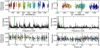 |
Fig. A.1. Rotation period analysis using MEarth (left panel) and ASAS-SN (right panel) photometric data. Top panel: RG715 broadband light curve (left panel) and V band light curve (right panel). The color of the datapoints indicates the observation epoch. Middle panel: GLS periodograms. The vertical green lines represent the orbital period of the planet at 13.35 days and the red dots the peak with the highest power at 63.9 days (left panel) and 64.7 days (right panel). Bottom panel: phased light curves using the rotationperiod derived from the GLS. The black curves show the best-fit sinusoidal models with an amplitude of 2.64 mmag (left panel) and 7.53 mmag (right panel). The black squares indicate the mean magnitude in ten equidistant bins in phase. |
Appendix B: MCMC cornerplots
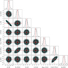 |
Fig. B.1. Two-dimensional projections of the posterior probability distributions of the circular single-planet Keplerian model. The contours represent the 1, 2, and 3σ uncertainty levels. |
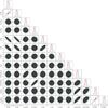 |
Fig. B.3. Same as Fig. B.1 but for the two-planet Keplerian model on circular orbits with a period ratio of 2:1. |
Appendix C: Radial velocities of GJ 4276
Barycentric Julian date, radial velocities, and formal uncertainties for GJ 4276.
References
- Anglada-Escudé, G., López-Morales, M., & Chambers, J. E. 2010, ApJ, 709, 168 [NASA ADS] [CrossRef] [Google Scholar]
- Baluev, R. V. 2009, MNRAS, 393, 969 [NASA ADS] [CrossRef] [Google Scholar]
- Barnes, S. A. 2007, ApJ, 669, 1167 [NASA ADS] [CrossRef] [Google Scholar]
- Bauer, F. F., Zechmeister, M., & Reiners, A. 2015, A&A, 581, A117 [NASA ADS] [CrossRef] [EDP Sciences] [Google Scholar]
- Berta, Z. K., Irwin, J., Charbonneau, D., Burke, C. J., & Falco, E. E. 2012, AJ, 144, 145 [NASA ADS] [CrossRef] [Google Scholar]
- Boisvert, J. H., Nelson, B. E., & Steffen, J. H. 2018, MNRAS, 480, 2846 [NASA ADS] [CrossRef] [Google Scholar]
- Caballero, J. A., Guàrdia, J., López del Fresno, M., et al. 2016, Proc. SPIE, 9910, 99100E [Google Scholar]
- Cortés-Contreras, M. 2016, PhD thesis, Universidad Complutense de Madrid, Spain [Google Scholar]
- Cumming, A., Marcy, G. W., & Butler, R. P. 1999, ApJ, 526, 890 [NASA ADS] [CrossRef] [Google Scholar]
- Czesla, S., & Schmitt, J. H. M. M. 2010, A&A, 520, A38 [NASA ADS] [CrossRef] [EDP Sciences] [Google Scholar]
- Díez Alonso, E., Caballero, J. A., Montes, D., et al. 2019, A&A, 621, A126 [NASA ADS] [CrossRef] [EDP Sciences] [Google Scholar]
- Dressing, C. D., & Charbonneau, D. 2015, ApJ, 807, 45 [NASA ADS] [CrossRef] [Google Scholar]
- Foreman-Mackey, D. 2016, J. Open Source Software, 24 [NASA ADS] [CrossRef] [Google Scholar]
- Foreman-Mackey, D., Hogg, D. W., Lang, D., & Goodman, J. 2013, PASP, 125, 306 [CrossRef] [Google Scholar]
- Gaia Collaboration (Brown, A. G. A., et al.) 2018, A&A, 616, A1 [NASA ADS] [CrossRef] [EDP Sciences] [Google Scholar]
- Gillon, M., Triaud, A. H. M. J., Demory, B.-O., et al. 2017, Nature, 542, 456 [NASA ADS] [CrossRef] [PubMed] [Google Scholar]
- Henry, T. J., Jao, W.-C., Subasavage, J. P., et al. 2006, AJ, 132, 2360 [NASA ADS] [CrossRef] [Google Scholar]
- Hobson, M. J., Díaz, R. F., Delfosse, X., et al. 2018, A&A, 618, A103 [NASA ADS] [CrossRef] [EDP Sciences] [Google Scholar]
- Husser, T.-O., Wende-von Berg, S., Dreizler, S., et al. 2013, A&A, 553, A6 [NASA ADS] [CrossRef] [EDP Sciences] [Google Scholar]
- Jackson, B., Greenberg, R., & Barnes, R. 2008, ApJ, 678, 1396 [NASA ADS] [CrossRef] [Google Scholar]
- Johnson, J. A., Payne, M., Howard, A. W., et al. 2011, AJ, 141, 16 [NASA ADS] [CrossRef] [Google Scholar]
- Kaminski, A., Trifonov, T., Caballero, J. A., et al. 2018, A&A, 618, A115 [NASA ADS] [CrossRef] [EDP Sciences] [Google Scholar]
- Kopparapu, R. K., Ramirez, R., Kasting, J. F., et al. 2013, ApJ, 765, 131 [NASA ADS] [CrossRef] [Google Scholar]
- Kopparapu, R. K., Ramirez, R. M., SchottelKotte, J., et al. 2014, ApJ, 787, L29 [NASA ADS] [CrossRef] [Google Scholar]
- Kürster, M., Trifonov, T., Reffert, S., Kostogryz, N. M., & Rodler, F. 2015, A&A, 577, A103 [NASA ADS] [CrossRef] [EDP Sciences] [Google Scholar]
- Lépine, S., Hilton, E. J., Mann, A. W., et al. 2013, AJ, 145, 102 [NASA ADS] [CrossRef] [Google Scholar]
- Luque, R., Nowak, G., Pallé, E., et al. 2018, A&A, 620, A171 [NASA ADS] [CrossRef] [EDP Sciences] [Google Scholar]
- Marcy, G. W., Butler, R. P., Fischer, D., et al. 2001, ApJ, 556, 296 [NASA ADS] [CrossRef] [Google Scholar]
- Mayor, M., Udry, S., Naef, D., et al. 2004, A&A, 415, 391 [NASA ADS] [CrossRef] [EDP Sciences] [Google Scholar]
- Nelder, J. A., & Mead, R. 1965, Comput. J., 7, 308 [CrossRef] [Google Scholar]
- Passegger, V. M., Reiners, A., Jeffers, S. V., et al. 2018, A&A, 615, A6 [NASA ADS] [CrossRef] [EDP Sciences] [Google Scholar]
- Protassov, R., van Dyk, D. A., Connors, A., Kashyap, V. L., & Siemiginowska, A. 2002, ApJ, 571, 545 [NASA ADS] [CrossRef] [Google Scholar]
- Quirrenbach, A., Amado, P. J., Ribas, I., et al. 2018, Proc. SPIE, 10702, 107020W [Google Scholar]
- Reid, I. N., Hawley, S. L., & Gizis, J. E. 1995, AJ, 110, 1838 [NASA ADS] [CrossRef] [Google Scholar]
- Reiners, A., Zechmeister, M., Caballero, J. A., et al. 2018a, A&A, 612, A49 [NASA ADS] [CrossRef] [EDP Sciences] [Google Scholar]
- Reiners, A., Ribas, I., Zechmeister, M., et al. 2018b, A&A, 609, L5 [Google Scholar]
- Ribas, I., Tuomi, M., Reiners, A., et al. 2018, Nature, 563, 365 [NASA ADS] [CrossRef] [Google Scholar]
- Rivera, E. J., Laughlin, G., Butler, R. P., et al. 2010, ApJ, 719, 890 [Google Scholar]
- Rodríguez, E., García, J. M., Costa, V., et al. 2010, MNRAS, 408, 2149 [NASA ADS] [CrossRef] [Google Scholar]
- Roeser, S., Demleitner, M., & Schilbach, E. 2010, AJ, 139, 2440 [NASA ADS] [CrossRef] [Google Scholar]
- Sarkis, P., Henning, T., Kürster, M., et al. 2018, AJ, 155, 257 [NASA ADS] [CrossRef] [Google Scholar]
- Schäfer, S., Guenther, E. W., Reiners, A., et al. 2018, Proc. SPIE, 10702, 1070276 [Google Scholar]
- Schmitt, J. H. M. M., Fleming, T. A., & Giampapa, M. S. 1995, ApJ, 450, 392 [NASA ADS] [CrossRef] [Google Scholar]
- Seager, S., & Mallén-Ornelas, G. 2003, ApJ, 585, 1038 [NASA ADS] [CrossRef] [Google Scholar]
- Shappee, B. J., Prieto, J. L., Grupe, D., et al. 2014, ApJ, 788, 48 [NASA ADS] [CrossRef] [Google Scholar]
- Skrutskie, M. F., Cutri, R. M., Stiening, R., et al. 2006, AJ, 131, 1163 [NASA ADS] [CrossRef] [Google Scholar]
- Steffen, J. H., & Hwang, J. A. 2015, MNRAS, 448, 1956 [NASA ADS] [CrossRef] [Google Scholar]
- Tinney, C. G., Butler, R. P., Marcy, G. W., et al. 2006, ApJ, 647, 594 [NASA ADS] [CrossRef] [Google Scholar]
- Trifonov, T., Kürster, M., Zechmeister, M., et al. 2017, A&A, 602, L8 [NASA ADS] [CrossRef] [EDP Sciences] [Google Scholar]
- Trifonov, T., Kürster, M., Zechmeister, M., et al. 2018, A&A, 609, A117 [NASA ADS] [CrossRef] [EDP Sciences] [Google Scholar]
- Vogt, S. S., Butler, R. P., Marcy, G. W., et al. 2005, ApJ, 632, 638 [NASA ADS] [CrossRef] [Google Scholar]
- Wilks, S. S. 1938, Ann. Math. Statist., 9, 60 [Google Scholar]
- Wittenmyer, R. A., Wang, S., Horner, J., et al. 2013, ApJS, 208, 2 [NASA ADS] [CrossRef] [Google Scholar]
- Wright, J. T., & Eastman, J. D. 2014, PASP, 126, 838 [NASA ADS] [CrossRef] [EDP Sciences] [Google Scholar]
- Zechmeister, M., & Kürster, M. 2009, A&A, 496, 577 [NASA ADS] [CrossRef] [EDP Sciences] [Google Scholar]
- Zechmeister, M., Kürster, M., & Endl, M. 2009, A&A, 505, 859 [NASA ADS] [CrossRef] [EDP Sciences] [Google Scholar]
- Zechmeister, M., Anglada-Escudé, G., & Reiners, A. 2014, A&A, 561, A59 [NASA ADS] [CrossRef] [EDP Sciences] [Google Scholar]
- Zechmeister, M., Reiners, A., Amado, P. J., et al. 2018, A&A, 609, A12 [CrossRef] [Google Scholar]
SpEctrum Radial Velocity AnaLyser, https://github.com/mzechmeister/serval
All Tables
Barycentric Julian date, radial velocities, and formal uncertainties for GJ 4276.
All Figures
|
Fig. 1. Rotation period analysis using SNO photometric data. Top panel: V band light curve. The color of the datapoints indicates the observation epoch. Middle panel: GLS periodogram. The vertical green line represents the orbital period of the planet at 13.35 days and the red dot the peak with the highest power at 32.3 days. Bottom panel: phased light curve using twice the period derived from the GLS. The black squares indicate the mean magnitude in ten equidistant bins in phase. |
| In the text | |
|
Fig. 2. Top panel: radial velocity measurements of GJ 4276 obtained with CARMENES as a function of barycentric Julian Date. The best-fit eccentric single-planet Keplerian model is overplotted in red (see Sect. 4.2). Bottom panel: O − C residuals. |
| In the text | |
|
Fig. 3. GLS periodograms of GJ 4276. Panel a: periodogram of the CARMENES RVs. The horizontal lines (dotted, dash-dotted, dashed) indicate FAP levels of 10%, 1%, and 0.1%. The vertical green line marks the orbital period with the highest power at 13.347 d. The left red dashed line at Prot = 64.3 d (frot = 0.0156 d−1) shows the weighted mean of the photometrically derived stellar rotation period and the right red dashed line its first harmonic (2frot = 0.0311 d−1). Panel b: periodogram of the residuals after removing the best-fit single-planet Keplerian with eccentricity (see Sect. 4.2.2) signal; panel c: window function of the RV data. Panels d–h: periodograms of the chromatic RV index (CRX), differential line width (dLW), as well as FWHM, contrast, and bisector span from the CCF analysis. Panels i–l: periodograms of the chromospheric line indices of Hα and Ca II IRT. |
| In the text | |
|
Fig. 4. Phase-folded radial velocity measurements of GJ 4276, together with the best-fit Keplerian model (black line) overplotted. In the bottom of each panel we show the O − C residuals. Top panel: circular single-planet Keplerian model. Middle panel: eccentric single-planet Keplerian model. Bottom panel: two-planet Keplerian model on circular orbits with a period ratio of 2:1. In addition, we show the best-fit Keplerian model of GJ 4276 b (green dashed line) and GJ 4276 c (red dotted line). |
| In the text | |
|
Fig. 5. Empirical distribution of the |
| In the text | |
|
Fig. 6. Histograms of the likelihood ratio using simulated data sets based on the best-fit eccentric single-planet model (solid red) and the circular two-planet model (dashed green). The vertical solid red line and the dashed green line represent the median values of the histograms. The black dotted vertical line represents the measured likelihood ratio
|
| In the text | |
|
Fig. 7. Eccentricity plotted against orbital period of known exoplanets around M dwarfs (dots). The colors indicate the minimum mass and the star marks the position of GJ 4276 b with the eccentric single-planet solution. |
| In the text | |
|
Fig. A.1. Rotation period analysis using MEarth (left panel) and ASAS-SN (right panel) photometric data. Top panel: RG715 broadband light curve (left panel) and V band light curve (right panel). The color of the datapoints indicates the observation epoch. Middle panel: GLS periodograms. The vertical green lines represent the orbital period of the planet at 13.35 days and the red dots the peak with the highest power at 63.9 days (left panel) and 64.7 days (right panel). Bottom panel: phased light curves using the rotationperiod derived from the GLS. The black curves show the best-fit sinusoidal models with an amplitude of 2.64 mmag (left panel) and 7.53 mmag (right panel). The black squares indicate the mean magnitude in ten equidistant bins in phase. |
| In the text | |
|
Fig. B.1. Two-dimensional projections of the posterior probability distributions of the circular single-planet Keplerian model. The contours represent the 1, 2, and 3σ uncertainty levels. |
| In the text | |
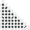 |
Fig. B.2. Same as Fig. B.1 but for the eccentric single-planet Keplerian model. |
| In the text | |
|
Fig. B.3. Same as Fig. B.1 but for the two-planet Keplerian model on circular orbits with a period ratio of 2:1. |
| In the text | |
Current usage metrics show cumulative count of Article Views (full-text article views including HTML views, PDF and ePub downloads, according to the available data) and Abstracts Views on Vision4Press platform.
Data correspond to usage on the plateform after 2015. The current usage metrics is available 48-96 hours after online publication and is updated daily on week days.
Initial download of the metrics may take a while.