| Issue |
A&A
Volume 622, February 2019
|
|
|---|---|---|
| Article Number | A97 | |
| Number of page(s) | 14 | |
| Section | Celestial mechanics and astrometry | |
| DOI | https://doi.org/10.1051/0004-6361/201834026 | |
| Published online | 05 February 2019 | |
Orbital stability of Earth Trojans
1
School of Astronomy and Space Science, Nanjing University, 163 Xianlin Avenue, Nanjing 210046, PR China
e-mail: zhouly@nju.edu.cn
2
Key Laboratory of Modern Astronomy and Astrophysics in Ministry of Education, Nanjing University, Nanjing 210046, PR China
3
Universitätssternwarte Wien, Türkenschanzstr. 17, 1180 Wien, Austria
Received:
5
August
2018
Accepted:
4
December
2018
The only discovery of Earth Trojan 2010 TK7 and the subsequent launch of OSIRIS-REx have motived us to investigate the stability around the triangular Lagrange points of the Earth, L4 and L5. In this paper we present detailed dynamical maps on the (a0, i0) plane with the spectral number (SN) indicating the stability. Two main stability regions, separated by a chaotic region arising from the ν3 and ν4 secular resonances, are found at low (i0 ≤ 15°) and moderate (24 ° ≤i0 ≤ 37°) inclinations, respectively. The most stable orbits reside below i0 = 10° and they can survive the age of the solar system. The nodal secular resonance ν13 could vary the inclinations from 0° to ∼10° according to their initial values, while ν14 could pump up the inclinations to ∼20° and upwards. The fine structures in the dynamical maps are related to higher degree secular resonances, of which different types dominate different areas. The dynamical behaviour of the tadpole and horseshoe orbits, reflected in their secular precession, show great differences in the frequency space. The secular resonances involving the tadpole orbits are more sensitive to the frequency drift of the inner planets, thus the instabilities could sweep across the phase space, leading to the clearance of tadpole orbits. We are more likely to find terrestrial companions on horseshoe orbits. The Yarkovsky effect could destabilize Earth Trojans in varying degrees. We numerically obtain the formula describing the stabilities affected by the Yarkovsky effect and find the asymmetry between the prograde and retrograde rotating Earth Trojans. The existence of small primordial Earth Trojans that avoid being detected but survive the Yarkovsky effect for 4.5 Gyr is substantially ruled out.
Key words: celestial mechanics / minor planets, asteroids: general / planets and satellites: individual: the Earth / planets and satellites: dynamical evolution and stability / methods: miscellaneous
© ESO 2019
1. Introduction
In the circular restricted three-body model for a massless asteroid moving in the gravitational field of the Sun and a planet, the equilateral triangular Lagrange equilibrium points, usually denoted by L4 and L5 for the leading and trailing point, respectively, are dynamically stable for all planets in our solar system (see e.g. Murray & Dermott 1999). Small celestial objects may find stable residence around these equilibrium points. The first such asteroid librating around the L4 point of Jupiter (588 Achilles) was discovered in 1906 by Wolf (1907). Nowadays several thousand objects are observed orbiting around either L4 or L5 point of the Earth, Mars, Jupiter, Uranus, and Neptune (see lists at International Astronomical Union: Minor Planet Center (MPC)1). These asteroids are called Trojans after the mythological story of the Trojan War. A Trojan asteroid shares the same orbit with its parent planet and in fact is locked in the 1:1 mean motion resonance (MMR) with the planet.
There have been many studies devoted to the Trojan dynamics (e.g. Mikkola & Innanen 1990, 1992; Nesvorný & Dones 2002; Scholl et al. 2004; Zhou et al. 2009, 2011; Lykawka et al. 2009, 2011; Ćuk et al. 2012). This topic is of special interest not only because a Trojan may exhibit complicated orbital behaviour, but also because the existence and properties of Trojans are the touchstone by which the viability of the scenarios proposed for the early evolution of our solar system (Morbidelli et al. 2005; Nesvorný & Vokrouhlický 2009) can be checked.
As for the Earth, observational searches for Trojans face unique difficulties due to the particular viewing geometry. The nearness of Trojans to the Earth leads to the wide area of sky to be searched. On the other hand, the location of Trojans close to the triangular Lagrange points place these objects in the daytime sky making the observations suffer higher airmass and the increased sky brightness of twilight (Wiegert et al. 2000). In 2010, a 300 m object (2010 TK7) was detected by the Wide-field Infrared Survey Explorer (WISE; Mainzer et al. 2011) and subsequently was confirmed to be the first Earth Trojan (Connors et al. 2011). At the same time, another candidate 2010 SO16 was identified as a horseshoe companion of the Earth (Christou & Asher 2011).
The asteroid 2010 TK7 lies in an eccentric and inclined orbit (e ∼ 0.19, i ∼ 21°) around the L4 point of the Earth. For its orbital elements, see for example Asteroids-Dynamic Site (AstDyS-2)2. Dvorak et al. (2012) demonstrated that the asteroid 2010 TK7 is situated out of the stability zone, leading to a total lifetime of being in the 1:1 MMR with the Earth less than 0.25 Myr. These authors also performed a numerical investigation of the phase space within a truncated planetary system from Venus to Saturn (Ve2Sa) and constructed a stability diagram for Earth Trojans adopting the maximum eccentricity as the stability indicator. They suggested that the apsidal secular resonances with Venus, the Earth, Mars, and Jupiter can be responsible for the structure of the dynamical map. However, perturbations from Uranus and Neptune could make some difference in the dynamical behaviour of Earth Trojans and the integration time of 10 Myr may not be long enough for the maximum eccentricity to indicate the long-term stability of these objects.
Tabachnik & Evans (2000) carried out numerical surveys on the fictitious Earth Trojans with a complete model including all of the planets in our solar system and found test particles can retain stable orbits at low (i ≲ 16°) and moderate (24 ° ≲i ≲ 34°) inclinations with their semi-major axis extending to 1 ± 0.012 AU. According to the investigations of Dvorak et al. (2012), the corresponding stability windows for inclinations are i ≲ 20° and 28 ° ≲i ≲ 40°, respectively. Moreover, they found a small U-shaped stability region around i = 50° (see Fig. 8 in Dvorak et al. 2012). Marzari & Scholl (2013) took the Yarkovsky force into account and purported that the most stable Earth Trojans can survive for a few Gyr, which means it could be possible to find primordial Trojans in the tadpole regions of the Earth.
This paper proffers a more detailed dynamical map of Earth Trojans and explores the significant resonances that carve the stability diagram. In Sect. 2, we introduce the dynamical model and numerical algorithm. In addition, we illustrate the method of the spectral analysis and explain how we obtain the proper frequency of fictitious Earth Trojans. In Sect. 3, we describe the dynamical maps on the plane of (a0, i0). With the help of these maps, we then determine the possible stability regions for Earth Trojans. In Sect. 4, we employ a frequency analysis method and derive the resonances that are responsible for the structures of the phase space. The influences of the Yarkovsky effect on Earth Trojans are discussed in Sect. 5. Finally, Sect. 6 presents the conclusions and discussions.
2. Model and method
2.1. Dynamical model and initial conditions
To investigate the orbital stability and dynamical behaviour of Earth Trojans, we numerically simulated their orbital evolution and then assessed their orbital stability by a method of spectral analysis. The dynamical model adopted in our simulations, which is referred to as Ve2Ne hereafter, consists of the Sun, all of the planets in our solar system except Mercury (from Venus to Neptune), and massless fictitious Earth Trojans (test particles). Mercury is excluded because it has negligible influence on the evolution of Earth Trojans in this research while the model including Mercury consumes much longer computation time (Dvorak et al. 2012). We adopted the Earth-Moon barycentre instead of the separate Earth and Moon as Dvorak et al. (2012) did. The initial orbits of the planets at epoch of JD 245 7400.5 are derived from the JPL HORIZONS system3 (Giorgini et al. 1996).
We initialized the orbital elements of the fictitious Trojans in a similar way as Dvorak et al. (2012). The test particles share the same eccentricity e, longitude of the ascending node Ω, and mean anomaly M with the Earth. The argument of perihelion ω0 is set as ω0 = ω3 ± 60°, where the triangular Lagrange points lie4. We sampled the initial semi-major axes and inclinations uniformly on the (a0, i0) plane to reveal their correlation with the stability. The semi-major axis ranges from 0.99 AU to 1.01 AU with an interval of 10−4 AU and the inclinations are varied from 0° to 60° in a step of 1°.
The Yarkovsky effect acting on a rotating body is a radiation force caused by the anisotropic thermal re-emission. Small objects, especially meteoroids and small asteroids undergo a semi-major axis drift under the perturbation of the Yarkovsky effect (Opik 1951). We performed an extra set of simulations to explore how the Yarkovsky effect influences the dynamical behaviour of Earth Trojans. We adopted a complete linear model proposed by Vokrouhlický (1999) to simulate the Yarkovsky effect in our calculations.
We implemented a Lie-series integrator (Hanslmeier & Dvorak 1984) to integrate the whole system. The hybrid symplectic integrator in the MERCURY6 software package (Chambers 1999) was also implemented for simulations including the Yarkovsky effect.
2.2. Spectral analysis
We applied a spectral analysis method in our orbital integrations to remove the short-period terms and reduce the amount of the output data. Furthermore, the method provides us an accurate stability indicator to construct the dynamical map in Sect. 3.1.
We employed an on-line low-pass digital filter (Michtchenko & Ferraz-Mello 1993, 1995) in smoothing the output of the preliminary integration, of which the interval is chosen to be 16 days. We then resampled the filtered data with an interval of Δ = 32 768 days (≈90 yr). The whole system is integrated for ∼1.2 × 10⁷ yr so that we obtain N = 217 (=131 072) lines of signal in time domain for further analysis.
A fast Fourier transform (FFT) is applied to the filtered data afterwards. The corresponding Nyquist frequency is fNyq = 1/(2Δ)=5.557 × 10−3 yr−1, which is larger than all the fundamental secular frequencies (see Sect. 4.1) in our solar system. The spectral resolution of the filtered data is fres = 1/(NΔ)=8.504 × 10−8 yr−1.
The spectral number (SN) is defined to be the number of the peaks over a specific threshold in a frequency spectrum (Michtchenko et al. 2002; Michtchenko & Ferraz-Mello 1995; Zhou et al. 2009, 2011). The SN could reflect the long-term stability within a relatively short integration time. We made use of the SN as stability indicator in our dynamical maps as Zhou et al. (2009, 2011) did for Neptune Trojans.
The critical angle (resonant angle) for a Trojan in the 1:1 MMR with the Earth is σ = λ − λ3, where λ = ω + Ω + M is the mean longitude. In this paper, we mainly use the SN of cosσ to construct the dynamical maps.
2.3. Numerical analysis of proper frequencies
Laskar (1990) introduced a method based on the evolution of the proper frequencies with time to analyse the stability in a conservative dynamical system. This so-called frequency map analysis (FMA) relies heavily on the accuracy of the determination of the proper frequency. A refined numerical algorithm that is several orders of magnitude more precise than the simple FFT was applied in FMA (Laskar 1990, 1993a,b; Laskar et al. 1992). For the high precision and feasibility, we implemented the same algorithm to define the proper frequencies of Earth Trojans. In this section we just outline the numerical algorithm.
Any given quasi-periodic function f(t) in the complex domain can be expressed in the form
where ak are the complex amplitudes (in descending order) of the corresponding periodic terms dominated by the frequencies ωk. This algorithm can numerically provide a precise recovery of f(t) over a finite time span [ − T, T],
The frequencies and amplitudes can be determined by an iterative scheme. At first, we conduct a modified FFT to f(t),
where χ(t) is a weight function that satisfies
As always, we use the Hanning window χ(t)=1 + cos(πt/T) as the weight function for reducing the aliasing. The value  can be estimated by searching for the maximum term of the amplitude function Ψ(ω). Then we refine the estimation of
  in its neighbourhood by maximizing Eq. (3) and the amplitude
  can be derived by orthogonal projection on
  .
.
The above steps are repeated on the new function  for the following frequency. Last but not least, we have to orthogonalize the basis
  every time a new frequency is determined.
The iteration can be stopped either when the desired number of the frequencies is reached, or when the amplitude associated with the last frequency falls below a specific noise level.
3. Dynamical map
Once the numerical integration is completed, an FFT is applied to the output. From the frequency spectrum of cosσ, we obtain the SN of each orbit on the (a0, i0) plane by counting the number of peaks that are higher than 1 per cent of the highest peak. As mentioned before, the smaller the SN is, the more regular the orbit is.
3.1. Dynamical map
We present the dynamical map around the L4 point on the (a0, i0) plane in Fig. 1. The colour represents the base-10 logarithm of SN, which now serves as an indicator of the orbital stability. Orbits in blue are of the greatest stability while those in red are very close to chaos. The orbits that dissatisfy 0.98 AU ≤ a ≤ 1.02 AU at any time in the integration are regarded as escaping from the 1:1 MMR and they are excluded in the dynamical maps. The criterion is derived empirically by inspecting the orbital evolution of Earth Trojans.
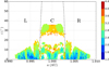 |
Fig. 1. Dynamical map around the L4 point on the (a0, i0) plane. The colour indicates the SN of cosσ, which is shown on a base-10 logarithmic scale for more details. The orbits that escape from the Earth co-orbital region (see text) during the integration time (12 Myr) are excluded. The dashed lines indicate the separatrices between the tadpole and horseshoe orbits (see text in Sect. 4.2), which divide the dynamical map into three regimes. The tadpole orbits reside in the central region (denoted by “C”) while the horseshoe orbits are found in the left (“L”) and right (“R”) regions. |
As can be seen from Fig. 1, the stability regions show an apparent symmetry about a0 ≈ 1 AU. For low inclinations, the stability window extends to ±0.0085 AU for semi-major axis centred at 1 AU, which is a bit broader than that of the coplanar orbits. Then the region shrinks with the increasing inclinations until i0 ≈ 15°, where an instability strip appears. For inclinations larger than 24°, a game-pad-shaped island spanning a range of 0.9975–1.0025 AU for semi-major axis is found to be able to hold stable orbits. In the region above 37°, no orbit can survive for 12 Myr as a co-orbiting companion of the Earth. Another point to note is that the stability regions are being eroded by instabilities. Two rifts stand at 1 ± 0.0028 AU, and serve to divide the dynamical map into three regimes. In the central area, a pair of white curves indicating escaped orbits lie around ±0.0015 AU about the centre while a V-shaped instability barrier is settled above them around i0 ≈ 10°. Besides, at the bottom of the stability island around i0 = 30°, some orbits are excited to give rise to the instability.
Left and right areas are symmetrical about a0 ≈ 1 AU and in each of these, there exists a triangular gap at the boundary of the stability region. The orbits surrounded by these instability strips could be endowed with SN over 104 (in red) and they escape from the Earth co-orbital region in the near future.
The most stable orbits of which the SN is smaller than 100 mainly reside in the region of i0 ≤ 10°. A further simulation up to 4.5 Gyr reveals that these orbits could survive the age of the solar system. We may most possibly observe Earth Trojans in slightly inclined orbits because they occupy the largest stable area in the phase space according to Fig. 1.
It is already known that phase spaces around the L4 and L5 points are dynamically identical to each other (see e.g. Zhou et al. 2009). We calculated the dynamical map around the L5 point and present it in Fig. 2. It is almost the same as that in Fig. 1, and no remarkable dynamical asymmetry between the L4 and L5 points can be found. As a result, we may investigate only one of these points, then the same conclusion can be applied to the other. In this paper we focus on the L4 point.
3.2. Region around i = 50°
At high inclinations (i ≳ 40°), Earth Trojans are trapped in the Kozai mechanism (Kozai 1962; Lidov 1962). As a result of the increasing eccentricity, the Trojans sustain close encounters with the planets, which give rise to instability (Brasser et al. 2004). For Earth Trojans at moderate inclinations, the ν3 and ν4 secular resonances may affect their orbits and increase eccentricity (Brasser & Lehto 2002). We note that in accordance with practice, we denote the secular resonance as νi when g = gi and ν1i when s = si, where g (gi) and s (si) represent the precession rate of the perihelion and ascending node of Trojans (planet).
Dvorak et al. (2012) adopted the maximum eccentricity as the stability indicator and constructed a similar stability diagram. In that investigation, a small stability region appears around i = 50°, which is unexpected according to our simulations. Considering the shorter integration time and the absence of Uranus and Neptune in the model Ve2Sa, we have to check the results simulated with different models for different integration times to verify the existence of the aforementioned stability region. We run four sets of simulations with different combinations of the model (Ve2Sa and Ve2Ne) and integration time (1 Myr and 12 Myr). The results are summarized in Fig. 3.
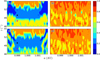 |
Fig. 3. Dynamical maps for the possible stability window around i = 50° (Dvorak et al. 2012) on the (a0, i0) plane. The colour indicates the maximum eccentricity during the integration time. The four panels stand for the results derived from different models and integration times: Ve2Sa and integrated for 1 Myr (panel a), Ve2Sa for 12 Myr (panel b), Ve2Ne for 1 Myr (panel c), and Ve2Ne for 12 Myr (panel d). The stars in panelsa and c indicate the initial conditions for the orbits shown in Fig. 4. Magenta, black, and red stand for (a0, i0)=(0.9990, 48 ° ), (0.9990, 50 ° ) and (0.9982, 53 ° ), respectively. |
The left two panels in Fig. 3 confirm that the stability window around i = 50° exists for both models for an integration time of 1 Myr. However, this stability structure shrinks as the integration time goes on and then completely disappears within 12 Myr (see panels b and d in Fig. 3).
The orbits in the blue regions, whose edges look very fragmentized, are supposed to possess a maximum eccentricity smaller than 0.3 within 1 Myr. Among these orbits, the most stable orbits with emax ≤ 0.2 are at both wings of the blue areas. As we can see from panels a and c, it seems that the inclusion of Uranus and Neptune does not prevent the formation of the stability window, but shapes its structure. For the model containing Uranus and Neptune, the stability region extends to lower inclinations while both sides of the region are reduced.
On a close inspection of the orbital evolution, we find the ν5 secular resonance gives a major push to the formation of the stability region. The ν2 and ν3 resonances could be involved to some extent. In addition, the ν7 and ν8 resonances should in some way be responsible for the differences between the structures for two models. As examples to show these mechanisms, we show in Fig. 4 the orbits with initial (a0, i0) indicated in Fig. 3 for both models.
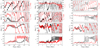 |
Fig. 4. Orbital evolution of the fictitious Trojans indicated in Fig. 3 for the model Ve2Sa (red) and Ve2Ne (black). From left to right, the three panels corresponding to the magenta, black, and red stars are of the initial conditions of (a0, i0)=(0.9990, 48 ° ), (0.9990, 50 ° ), and (0.9982, 53 ° ). We illustrate the temporal evolution of e, Δϖ5, and i for both models, Δϖ7, Δϖ8, and ω for the model Ve2Ne only and Δϖ2, Δϖ3, ΔΩ2, and ΔΩ3 for the model Ve2Sa only. The vertical dashed lines in the bottom plots of each panel indicate the lifespans of the orbits being in the 1:1 MMR. |
For model Ve2Sa, Δϖ2, Δϖ3, and Δϖ5 all librate more or less between 0°–360° for a period of time, where Δϖj = ϖ − ϖj is the difference in the longitude of perihelion between the asteroid and some planet that is labelled with the subscript j. For model Ve2Ne, besides the aforementioned three critical angles, Δϖ7 and Δϖ8 show librations as well.
Given the secular critical angle, the time variation of the eccentricity can be estimated by the linear theory of secular perturbation, which gives (e.g. Murray & Dermott 1999; Li et al. 2006)
where n and m represent the mean motion and mass with the subscript j indicating the planet. The parameter M⊙ is the mass of the Sun and  is a positive Laplace coefficient. Since C1 is negative, de/dt is negative when 0 ° < Δϖj < 180° and positive when 180 ° < Δϖj < 360°.
In consideration of the way in which the eccentricities evolve, we find that the ν5 secular resonance, which is characterized by a libration of Δϖ5, dominates the evolution of the eccentricities for both models. For model Ve2Sa, Δϖ5 of the most stable orbits at the blue wings librate around values ∼180°. Under the influence of ν5, the eccentricities of these orbits almost stay unchanged according to Eq. (5). For the less stable orbits in the middle area, the libration centre could exceed 180° and thus the eccentricities should undergo a secular increment. However, the participation of the ν2 and ν3 triggers the overlap of the secular resonances and chaos arises. Therefore, the orbits in the i = 50° region could hardly survive a lifespan longer than 6 Myr.
As shown in Fig. 4, for model Ve2Ne, Δϖ7 and Δϖ8 librate when the orbits remain in the Trojan clouds of the Earth. The inclusion of Uranus and Neptune sets the stage for the ν7 and ν8 secular resonances, which could further intensify the resonance overlap. Hence, the stability of the former blue areas could be reduced. Nevertheless, the perturbations from Uranus and Neptune could affect the precession of Jupiter. In some cases, the ν5 secular resonance can be maintained or even strengthened and that may also give rise to the extended stability region of low inclination.
The variations of the inclinations are likely under the control of the ν12 or ν13 secular resonances (see the middle and right panels of Fig. 4). The ν16 could be involved as well. The map of the variation of inclination reflects some structures similar to those for the maximum eccentricity.
From the right panel of Fig. 4 we find that the Kozai mechanism would be likely to take place once the orbits leave the ν5 secular resonance. In the Ve2Ne model (black lines), the orbit leaves the Trojan area due to a quick increase of eccentricity around 1.45 Myr, which is accompanied by a simultaneous decrease of inclination. This is the typical behaviour of orbits affected by the Kozai mechanism. The argument of perihelion ω could librate around ±90° and the inclination varies in exchange of the eccentricity to keep the Delaunay variable  constant.
3.3. Excitation of the eccentricity and inclination
The instability and escape of orbits in the Trojan region may be caused by various mechanisms, especially secular resonances. Among those survived orbits, various dynamical mechanisms may also excite their eccentricities and inclinations. Figure 5 shows the maximum eccentricity during orbital evolution on the (a0, i0) plane. Owing to the longer integration time, the instability strips in Fig. 5 are much broader than those found in previous study (Fig. 8 in Dvorak et al. 2012).
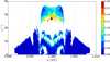 |
Fig. 5. Maximum eccentricity (in different colours) during orbital integrations of 12 Myr on the (a0, i0) plane. We show only for i0 ∈ [0 ° ,40 ° ] because there are no stable orbits with i0 > 37°. The black star stands for an orbit of (a0, i0)=(0.9999, 27 ° ) that is shown in Fig. 6. |
Figure 5 suggests that most survived orbits obtain a maximum eccentricity smaller than 0.09 during the integration time except those in the central area. Especially, the eccentricity of the orbits at the bottom of the island around i = 30° could reach its peak at 0.30, making it possible for them to encounter with other planets thus escape from the Earth co-orbital region in future.
To find out the involved secular resonances exciting the eccentricity, we check several possible critical angles. A preliminary inspection suggests that the ν4 secular resonance governs the motion of the orbits at the bottom of the stability island around i = 30°. The ν2 and ν3 resonances librate off and on during the whole life of these orbits. These mechanisms could act together to drive the eccentricity up with an upper limit of ∼0.25. The larger eccentricity up to ∼0.3 can be excited by the Kozai mechanism or some higher-degree secular resonances (see Sect. 4.4) and as a result, the orbits undergo close encounters with other planets and escape from the 1:1 MMR finally. As an example, we illustrate the evolution of such an orbit in Fig. 6. In fact, the survived orbits with the largest eccentricities in the stability island are of relatively large SN, which means they may leave the co-orbital region in tens of millions years and they also have a chance to be captured by the Kozai mechanism therein, just like the orbit shown in Fig. 6.
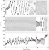 |
Fig. 6. Orbital evolution of the fictitious Earth Trojan indicated in Fig. 5 with the initial condition of a0 = 0.9999 AU, i0 = 27°. From top to bottom panels: evolutions of the apsidal differences between the Trojan and Mars Δϖ4, the argument of the perihelion ω and eccentricity e. The red vertical dashed lines in the bottom panel indicate the lifespan of the orbit. |
The variation of inclination during the integration time is presented in Fig. 7 on the (a0, i0) plane, which clearly shows that most Trojans cannot be excited to high-inclined orbits. Two distinct vertical strips indicating the largest variations of inclinations are on the edge of the triangular instability gaps. Apparently, the orbits in the red strips are protected by some strong resonances, which could excite the inclinations as well. It is worth noting that for the orbits with i0 < 20°, the variations of the inclinations may depend on their initial inclinations. These follow a positive correlation and the inclinations of the coplanar orbits are the hardest to be excited.
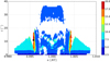 |
Fig. 7. Same as Fig. 5 but colours indicate the variation of inclinations. The black star stands for an orbit of (a0, i0)=(0.9958, 11 ° ) on the initial plane that is shown in Fig. 8. |
As well known, the secular resonances related to the apsidal and nodal precession may excite the eccentricity and inclination, respectively. Similar to the variation of the eccentricity mentioned before in Eq. (5), the evolution of the inclination can be described by (e.g. Murray & Dermott 1999; Li et al. 2006)
where  is another positive Laplace coefficient and hence C2 is a positive number for prograde orbits. As a result, di/dt is positive when 0 ° < ΔΩj < 180° and negative when 180 ° < ΔΩj < 360°.
We check the possible nodal secular resonances carefully and find that the critical angle ΔΩ3 of the coplanar orbits librates around 0° with extremely small amplitudes, thus their inclinations oscillate to a well limited extent. The amplitude of ΔΩ3 climbs towards the peak as the initial inclination increases until i0 ∼ 3°, from which the angle ΔΩ3 starts to circulate. The orbits in cyan at both wings of the stability region in Fig. 7 may be sheltered by some higher degree secular resonances (see Sect. 4.4) that could drive their inclinations up at the same time.
The ν14 secular resonance is dominant in exciting the inclinations to a level above 20°. As an example, Fig. 8 shows that the critical angle ΔΩ4 of such an orbit could librate between 0° and 180° for some time and the inclination oscillates correspondingly following the rule in Eq. (6). The inclination could reach its peaks at ∼20° within 2 Myr and then oscillates with a secular period of ∼2.7 Myr. Unlike in the Kozai mechanism, in this case the large variation of inclination is dissociated with the eccentricity and orbits in the corresponding region just maintain small eccentricities as shown in Fig. 5.
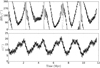 |
Fig. 8. Evolutions of the nodal differences between the Trojan and Mars ΔΩ4 (top panel) and inclination i (bottom panel) of the fictitious Earth Trojan indicated in Fig. 7 with the initial condition of a0 = 0.9958 AU, i0 = 11°. |
Actually, some higher degree secular resonances also play an important role in sculpting the dynamical map. With the aim of probing all possible resonances responsible for the stability of Earth Trojans, we conduct the frequency analysis in the next section.
4. Frequency analysis
Much valuable information lying behind the motions deserves to be mined as it points the way to locating the related secular and secondary resonances. In this section we follow the frequency analysis method proposed in Zhou et al. (2009, 2011) to portray the resonances. For each orbit in our simulations, several of the most significant frequencies with the largest amplitudes of cosσ, ecosϖ, and icosΩ are calculated using the technique introduced in Sect. 2.3. Then the proper frequencies indicating the precession rates are picked out and denoted by fσ, g, and s, respectively.
4.1. Dynamical spectrum
Generally, the spectra consisting of the forced frequencies, free frequencies, their harmonics, and combinations thereof are complicated. Fortunately, the proper frequencies stand out in continuous variations along some orbital parameters while the forced frequencies basically remain unchanged.
In our investigation, we vary the semi-major axes of the fictitious Earth Trojans with other orbital parameters fixed and record several leading frequencies for each orbit. We obtain the so-called dynamical spectrum if we plot all these frequencies against their initial semi-major axes. The dynamical spectra of icosΩ and ecosϖ for each initial inclination are calculated and two examples are shown in Fig. 9. The value i0 = 2° is selected to be illustrated arbitrarily as examples. We also take into account that the stability region at low inclination is wide (see Fig. 1) such that the corresponding dynamical spectra are expected to be relatively “clearer” for illustration. As we can see, the proper frequencies vary continuously with the semi-major axis while the forced frequencies derived from the perturbers hold the line. The fundamental secular frequencies in our solar system have been calculated with different models and methods in many works (e.g. Carpino et al. 1987; Nobili et al. 1989; Laskar 1990; Lhotka & Dvorak 2006). In this paper we refer to the results computed by Nobili et al. (1989) and Laskar (1990; Table 1). From the adopted fundamental frequencies, we identify the forced frequencies in the top panel as |s6|, |s3|, |s4| and 2g7 − s5. For the bottom panel, the forced frequencies are determined to be g4, g3 + s3 − s4, g2 and g5.
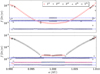 |
Fig. 9. Dynamical spectra of icosΩ (top panel) and ecosϖ (bottom panel) for orbits with initial inclinations i0 = 2°. The five most significant frequencies for each orbit are plotted against their initial semi-major axes. The frequencies with the largest amplitudes are labelled by red open circles while the second to the fifth are denoted by black open inverted triangles, squares, triangles, and diamonds, respectively. The blue dashed lines indicate the absolute values of the fundamental frequencies identified to be corresponding to forced frequencies. From top to bottom, they represent |s6|, |s3|, |s4|, 2g7 − s5, g4, g3 + s3 − s4, g2, and g5 respectively. We note that s3 and s4, (g3+s3−s4) and g4 are so close to each other that they are hardly distinguishable in the figure. Moreover, for a better vision, we just plot one-third of the data. |
Fundamental secular frequencies in the solar system except for Mercury.
Retrograde precession implies negative frequency values. The fundamental frequencies sj corresponding to the nodal precession rates of the planets are all negative. However, all frequencies we obtain by the numerical analysis should be positive in principle, so we have to monitor the variations of the longitude of perihelion and the longitude of ascending node to determine the sign of g and s for each fictitious Trojan.
The proper frequencies are not necessarily those with the largest amplitudes (red open circles in Fig. 9). The motions could be governed by some forced frequencies just like the orbits on both sides in the bottom panel, which are dominated by the nodal precession of Venus with g2 = 5.753 × 10−62π yr−1.
A linear secular resonance occurs every time the proper frequency g or s comes across the fundamental frequencies. High-degree resonances involving the combinations of secular frequencies can be determined in a similar way. However, the dynamical spectra could not always be as clear as the examples in Fig. 9. Actually, orbital chaos could make the dynamical spectra so complicated that we can only pick out the proper frequencies accurately in a limited area. Another noticeable feature in Fig. 9 that is discussed in the following section is that the proper frequencies seem to be divided into three regimes and are actually separated by the boundary between the tadpole and horseshoe orbits. This feature is more obvious for ecosϖ and cosσ but a close inspection proves it is valid for all three variables.
4.2. Tadpole and horseshoe orbits
For the planar circular restricted three-body problem, the test particles with small eccentricities are presumed to move in tadpole orbits if their orbits satisfy the equation (Murray & Dermott 1999)
where δr is the radial separation of the particles from the secondary mass, whose mass fraction and semi-major axis are denoted by μ and a. For the Sun-Earth system, μ ≈ 3 × 10⁻⁶ and a = 1 AU, thus δr ≈ 0.00283 AU. We recall the phase portrait (see Fig. 2 in Dvorak et al. 2012) derived from the symplectic mapping method and we get the same criterion considering δr ≈ δa for near-circular orbits. Weissman & Wetherill (1974) demonstrated that the tadpole orbits could be found within 0.00285 AU away from the Earth while the horseshoe regime extends to 1 ± 0.0080 AU. A larger horseshoe orbit could rapidly lose its stability because of the close approach to the Earth near the turning points.
In our study we were able to check the variation of the critical angle σ = λ − λ3 of the 1:1 MMR for each stable orbit from the output of the simulation to determine whether or not the orbit is in the tadpole regime. Actually another way taking advantage of the frequency analysis is preferred in practice to define the separatrices. We numerically calculate the spectrum of the variable cosλ for each orbit and record the dominant frequency of which the amplitude is the largest. For tadpole orbits the dominant frequency should exactly equal that of the mean motion of the Earth while the dominant frequency for horseshoe orbits could differ from the orbital frequency of the Earth owing to their elongated trajectories, which are farther away from the Earth. We adopt the above criterion and locate the critical semi-major axis for different inclinations. A numerical fit of the separatrices are
where alow and aup represent the lower and upper limit of the semi-major axis for tadpole orbits.
The separatrices between the tadpole and horseshoe orbits are shown in Fig. 1 utilizing Eq. (8). Obviously, the separatrices perfectly fit the instability rifts around 1 ± 0.0028 AU in the dynamical map. As we know, motions near the separatrix in the perturbed system are so chaotic that the instabilities arise there. Moreover, recall Fig. 9 and we find the proper frequencies undergo piecewise changes along semi-major axes. The variation trends are nearly symmetrical in regions L and R while they appear greatly different for tadpole orbits in region C. In the stability island around 30° where the high-inclined orbits could survive the integration time (∼12 Myr), all fictitious Trojans are in tadpole orbits.
4.3. Empirical formulae
Expressions of the proper frequencies g and s on the plane (a0, i0) are necessary for constructing the resonance maps. We pick out the orbits whose proper frequencies can be accurately determined and obtain the empirical formulae by numerical fitting. In order to reduce the round-off error, we normalize a0 and i0 of the selected orbits as  and
and  , where
  ,
,  and σa0, σi0 represent the mean value and standard deviation of the initial elements, respectively (Table 2).
Mean values and standard deviations of a0 (in AU) and i0 (in degree) of the orbits selected for the numerical fitting for g and s, respectively in regions L, C, and R.
We adopt the quintic polynomial as follows:
The coefficients pmn of the best fits for three different regions are listed in Table 3. We fit the proper frequencies in regions L and R separately to improve precision although they seem symmetrical about a0 ≈ 1 AU. Only the proper frequencies of the regular orbits can be determined accurately and used for the numerical fitting. In the white areas between the stability regions, where chaos arises, the empirical formulae are less reliable because the frequency spectra of those orbits are disordered and the proper frequencies can only been gained by interpolating. In the marginal area far away from the stability regions, the proper frequencies derived from the empirical formulae are suggested for reference only owing to a complete extrapolation.
Coefficients of the best fits for the proper frequencies g and s (in 2π yr−1) in regions L, C, and R on the (a0, i0) plane.
4.4. Secular resonances
With the help of the empirical formulae, the secular resonances can be determined by solving the equation
where p, q, pj, qj are integers. The d’Alembert rules require  and
and  must be even. The equation
  is defined as the degree of the secular resonance.
A complete search of the combinations of p, pj, q, and qj for different degrees identifies the secular resonances responsible for the structures in the dynamical maps. Figure 10 presents the main linear secular resonances on the (a0, i0) plane. Apparently, the orbits in the 15 ° ∼24° instability gap are likely governed by the apsidal secular resonances ν3 and ν4. Examinations of the critical angles reveal that the ν4 secular resonance has a stronger influence on the motions there. The nodal secular resonances ν13 and ν14 locate exactly where the inclinations are excited. As mentioned in Sect. 3.3, the ν13 could control the variations of the inclination depending on the initial values while the ν14 could drive the inclinations up to ∼20°. The ν6 resonance corresponds to an elongated instability strip where the eccentricity can be elevated. To a lesser extent, the ν16 contributes to the formation of the vertical strips of stability in the dynamical map.
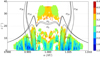 |
Fig. 10. Locations of main linear secular resonances for Trojans around the L4 point on the (a0, i0) plane. The resonances are labelled along the curves. |
These linear secular resonances have strong influences on the orbital evolution of Earth Trojans and they form the major structures in the dynamical map in a relatively short time. Still, there are rich fine structures in the dynamical map, arising from higher order secular resonances. As examples, we depict some major secular resonances below.
The main fourth-degree secular resonances are shown in Fig. 11 and the meaning of the labels along the curves are listed as follows:
 |
Fig. 11. Locations of the fourth-degree secular resonances for Trojans around the L4 point on the (a0, i0) plane. The resonances are labelled (see text for the meaning) along the curves. In consideration of the frequency drift of the inner planets, the dashed lines in the left panel delimit the possible locations of S4_A and G4_F (see Sect. 4.5). The black and red dashed lines represent the results derived from the data taken from Laskar (1990) and our integration, respectively. |
The resonances with q = 0 are classified as “G” type while those with p = 0 are classified as “S” type. They represent the secular resonances only involving the precession rates of the perihelion longitudes (g) and ascending nodes (s) of Earth Trojans, respectively. The others are denoted by “C” type in the name of “combined”.
As we can see in Fig. 11, the recognized secular resonances could match the fine structures of the dynamical maps well. The resonance overlap sets the border of the stability region for orbits with moderate inclinations. In the central areas, secular resonances such as G4_F can help block the way of the stability region towards higher inclinations. The orbits in the central instability areas are mainly subjected to C-type and G-type secular resonances although a few S-type resonances such as S4_A may be involved as well. The vertical strips in the regions L and R of the dynamical map indicating the most stable orbits should be related to the S-type secular resonances. The green gaps around 1 ± 0.006 AU splitting two blocks of the most stable orbits are an obvious example. The secular resonance S4_C involving the nodal precession of the Earth, Mars, and Jupiter could destabilize the orbits in these gaps slightly. To the contrary, there may exist some other resonances that improve the stability. The competition between the protection and destruction provided by the secular resonances result in the fragmentation in shape of the dynamical map.
In Fig. 12 we illustrate the main sixth-degree secular resonances and these are explained as follows:
Each fine structure could be shaped by multiple resonance mechanisms and actually, we just show in Figs. 11 and 12 some representatives of the resonance families whose strengths are relatively great. The secular resonances in the same family share the similar locations and they work together to control the motions of Earth Trojans, such as G4_F and C6_G, G4_B and C6_J, and C4_A and C6_E. What also needs to be emphasized is that each resonance has a width in which the orbits can be influenced effectively. The resonance width varies greatly for different resonances such that it is not always possible to distinguish the dominant resonances in fact.
The inclusion of Uranus and Neptune completes the secular resonance net shown above. On the one hand, Uranus and Neptune directly affect the Trojans as they are involved in many secular resonances although most of these are not plotted in Figs. 11 and 12; on the other hand, the perturbations from Uranus and Neptune act on the motion of Jupiter and Saturn, causing a modification to the dynamical behaviour of the Trojans.
In this paper we focus on the secular resonances and no secondary resonance has been shown. Some resonances contributing to the motions may not be included in the map either because they are located outside the (a0, i0) area. However, they can still influence the orbits within the resonance width in varying degrees, just like the ν5 resonance. According to Fig. 9, the ν5 secular resonance has a great influence on some Trojans although it resides outside the (a0, i0) area (Fig. 10). On the contrary, some resonances also have a chance not to occur near the locations derived from the empirical formulae if the orbits are affected more strongly by other mechanisms.
The typical lifetime of Earth Trojans trapped in a secular resonance is 1 Myr while the typical Lyapunov time could be 1 kyr (Brasser & Lehto 2002). The integration time in our simulations (∼12 Myr) is long enough for the Trojans governed by some secular resonance causing instabilities to escape from the 1:1 MMR region. Moreover, considering the frequency drift of the inner planets causing the shift of the secular resonances (see next subsection), the short typical lifetime of 1 Myr could facilitate the expansion of the instabilities.
4.5. Frequency drift of the inner planets
Chaotic motion with a maximum Lyapunov exponent of ∼1/5 Myr−1 was detected in the inner solar system by Laskar (1989) and they found this motion is related to the transition from libration to circulation of the critical angle of the secular resonance 2(g4−g3) − (s4−s3) = 0 (Laskar 1990). As a consequence, the secular frequencies of the inner planets keep changing to make the related secular resonances sweep across a large area of the phase space over a long time span.
The mean values and amplitudes of the variations of the fundamental secular frequencies for Venus, the Earth, and Mars are listed in Table 4 (Laskar 1990). These were obtained from numerical computations over 200 Myr, therefore the values of Δν in this case just set a lower limit of the frequency drift. Actually, we integrated the solar system to 1 Gyr and we find the frequency drift could be several times higher than the values obtained by Laskar (1990). However, we still refer to the data taken from Laskar (1990) to avoid conflict with the adopted fundamental frequencies.
Mean values ( ) and amplitudes of the variations (Δν) of the fundamental secular frequencies in the inner solar system, except for Mercury, over 200 Myr.
As we can see from Table 4, the variations of g3, g4, and s2 exceed 1.3 × 10⁻⁷ 2π yr−1, which could have a great influence on the sphere of resonant action. Roughly assuming the proper frequencies of Trojans are independent of the fundamental frequency drift, we define the boundary of the secular resonances by maximizing or minimizing  in Eq. (10) with the variations listed in Table 4. We note the mean value
  in this case differs a small amount from the frequencies in Table 1 that is calculated from a time window of 20 Myr. For example, the black dashed lines in the left panel of Fig. 11 define the coverage areas of the S4_A and G4_F resonances in consideration of the frequency drift. Apparently, shifts of the locations of these two resonances are remarkable, especially in region C, although we just give a lower limit of Δν. For a longer integration time, we get larger variations of the fundamental frequencies and thus the secular resonances could sweep across a broader area that is delimited by the red dashed lines. The absolute values of g and s in region C are much smaller than those in regions L and R (cf. Fig. 9), hence the locations of the secular resonances acting on the tadpole orbits are more sensitive to the frequency drift.
From Figs. 10–12 we can see that there exist numerous C-type and G-type secular resonances inducing instabilities in region C and most of these are related to the fundamental frequencies in the inner solar system. As the secular frequencies of the inner planets drift, the instability strips induced by the C-type and G-type secular resonances sweep across the phase space in region C. Finally, on a timescale of 4.5 Gyr, as long as the age of the solar system, chaos occupies most of the central areas, including the blue areas where the most stable Trojans reside (see the left panel in Fig. 11 for example), and then almost no tadpole orbits remain. In other words, there may be few primordial Earth Trojans on tadpole orbits. However, most of the horseshoe orbits with the smallest SN could survive the age of the solar system as the S-type secular resonances excluding s2 are hardly affected by the frequency drift. In view of the enormous amount of the potential extremely stable horseshoe orbits according to Fig. 1 (in blue), we may find abundant primordial terrestrial companions on horseshoe orbits.
5. Yarkovsky effect
5.1. Surviving ratio
The Yarkovsky effect can produce a thermal thrust on asteroids orbiting the Sun, resulting in the long-term evolution of the semi-major axis for small objects with diameter D = 0.1 m to ∼40 km (Bottke et al. 2006). For Earth Trojans, the Yarkovsky effect may make a great difference in their evolution due to the appropriate size and close distance to the Sun. To figure out the modification to the stability by the Yarkovsky effect, we selected a sample of 986 orbits whose lifespans are longer than 1 Gyr out from the 2870 orbits that survive in the ∼12 Myr integration to make the dynamical map (coloured points in Fig. 1). We then statistically analysed their dynamical behaviour under the Yarkovsky effect of various magnitudes that are determined by the distance to the Sun, the obliquity of the spin axis, and physical properties such as size and spin rate. As the diurnal component is much more remarkable than the seasonal component in our study, we just include the former in our computations.
According to Nesvorný et al. (2002), Bottke et al. (2006), and Marzari & Scholl (2013), we parameterize the Earth Trojans with a bulk density of 2.5 g cm−3, a surface density of 1.5 g cm−3, a surface conductivity of 0.001 W/(mK), an emissivity of 0.9, an albedo of 0.18, and the specific heat capacity of 680 J kg−1 K−1. Based on these parameters, we approximate and simplify the formula for the diurnal Yarkovsky effect developed by Vokrouhlický (1999) as
where ω, γ, and R represent the spin rate, obliquity of the spin axis, and radius of the asteroid, respectively. The da/dt, R, and ω are in AU/Gyr, metre and 2π s−1, respectively while γ ranges from 0° to 180°. For typical spin rate in the solar system, as mentioned in Bottke et al. (2006), ω ∼ 2π/(5R), we obtain
As mentioned before, the diurnal Yarkovsky effect depends on a variety of physical quantities, and different combinations of these parameters may lead to the same effect, so we exert different drift rates  on Earth Trojans instead of varying physical quantities in practice to avoid the degeneracy of the specific characteristics. After some tests the drift rates range from −4 AU/Gyr to 4 AU/Gyr, where the negative values indicate the retrograde spin (cosγ < 0 in Eq. (14)) and the positive values indicate the prograde spin. It should be noted that
  in this work refers to the derivative of Kepler orbital element, so it can be considered as an equivalent force. We therefore exert the equivalent forces with different strengths on each of the 986 Trojan orbits, and check whether they can stay in the 1:1 MMR under the semi-major axis drift due to Yarkovsky effect. Limited by the computing resource, we integrate the system to 1 Gyr. We count the number of survived Trojans during the integrations, compute the ratio of these to all 986 selected orbits, and present the results in Fig. 13.
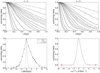 |
Fig. 13. Surviving ratio against evolution time for prograde spinning Trojans ( |


Surely the strongest Yarkovsky effect severely destabilizes the orbits and leads to the clearance of Earth Trojans. However, the larger size and slower rotation the Trojans are the weaker the Yarkovsky effect is. The surviving ratio p of affected Trojans must change with the drift rates  as well as the evolution time t, as the plots in Fig. 13 clearly show. For any given
  , empirically, we suppose the surviving ratio p decreases with time t following the rule below:
![$$ \begin{aligned} p=\exp \left[\alpha \, t^\beta \right], \end{aligned} $$](/articles/aa/full_html/2019/02/aa34026-18/aa34026-18-eq48.gif)
where  and
and  are coefficients depending on
  . We then find that α and β can be well fitted by
![$$ \begin{aligned} \begin{aligned} \alpha&=-\left(b_1 \dot{a}+b_2 \dot{a}^2+b_3 \dot{a}^3+b_4 \dot{a}^4\right), \\ \beta&=c_1\exp [c_2 \dot{a}] + c_3 \exp [c_4\dot{a}], \end{aligned} \end{aligned} $$](/articles/aa/full_html/2019/02/aa34026-18/aa34026-18-eq52.gif)
where bj, cj (j = 1, 2, 3, 4) are coefficients of the best fit. The solid curve in the lower left panel of Fig. 13 stands for such a fitting function  for t = 1 Gyr, and it matches the points obtained from integrations fairly well. Encouraged by this consistence, we also present an extrapolation of Eq. (15) to t = 4.5 Gyr (the dashed line), which gives an estimation of the surviving ratio of Earth Trojans at the age of the solar system.
Combining Eqs. (14) and (15), we get the expression of p(cos2/3γ/R, t). Taking the size of 2010 TK7 (∼300 m in diameter) into consideration, we calculate the surviving ratio after 1 Gyr evolution under the Yarkovsky effect and find p = 0.034 for the exactly retrograde rotation (γ = 180°) and p = 0.20 for the exactly prograde rotation (γ = 0°). At the age of 4.5 Gyr, the surviving ratio p reduces significantly. We display p against cos2/3γ/R at t = 4.5 Gyr in the lower right panel of Fig. 13. Now for Earth Trojans of 300 m in size, we find p = 5.4 × 10⁻²¹ for γ = 180° and p = 2.7 × 10⁻⁷ for γ = 0° (red crosses in Fig. 13), both practically approaching zero. In other words, the primordial Earth Trojans as large as 2010 TK7 must have been driven out from the 1:1 MMR by the Yarkovsky effect unless their spin axes lie almost in the orbital plane, where the seasonal (but not diurnal) component of the Yarkovsky effect dominates.
If we take the surviving ratio of 1% as the cut-off probability, the critical values of cos2/3γ/R for Earth Trojans having retrograde and prograde spin after 1 Gyr evolution are −7.68 km−1 and 11.1 km−1, which means that the smallest radius of Earth Trojans that survive for 1 Gyr in the 1:1 MMR is 130 m and 90 m, respectively, for the exactly retrograde (γ = 180°) and prograde rotators (γ = 0°). For primordial Earth Trojans, the evolution time t = 4.5 Gyr changes these two numbers to 400 m and 278 m, corresponding to absolute magnitude H = 18.00 and 18.79 if an albedo 0.18 is adopted.
Of course, if another albedo is adopted, or if the spin axis of Earth Trojans is not perpendicular to the orbital plane, the critical size of Earth Trojans that survive the Yarkovsky effect could be different. Suppose three different albedos (α), of which α = 0.1 is that of 2010 TK7 (Connors et al. 2011), α = 0.05 for C-type asteroid, and α = 0.25 for S-type asteroid, we calculate the critical absolute magnitudes of prograde and retrograde spinning Earth Trojans that can survive for 1 Gyr and 4.5 Gyr under the Yarkovsky effect and list these in Table 5.
Upper limits of absolute magnitudes (H) of Earth Trojans of various albedos (α) surviving for 1 Gyr and 4.5 Gyr.
We note that the magnitudes listed in Table 5 are the upper limits. For example, H(4.5 Gyr)=19.4p/18.6r for α = 0.10 means that any Earth Trojan of albedo 0.10 must be brighter than H = 19.4/18.6 if it is a prograde/retrograde rotator so that it is large enough in size to survive the Yarkovsky effect for the age of the solar system.
When the spin axis tilts away from the normal direction of the orbital plane, the Yarkovsky effect declines. Setting a detection limit of Earth Trojans as H = 20.5 (Cambioni et al. 2018), we calculate the possible obliquity of Earth Trojan that can survive for 4.5 Gyr and list the results in Table 5 for reference. Again, for α = 0.1 as 2010 TK7, any primordial Earth Trojan fainter than H = 20.5 must have an obliquity γ ∈ (67 ° ,103 ° ).
5.2. Asymmetry of the stability
As shown in Fig. 13, the surviving ratio displays an obvious asymmetry about  . With the same drift rate
  and at the same evolution time t, the orbits in prograde rotation are more likely to be stable than those in retrograde rotation. This asymmetry comes from the combined effect of the 1:1 MMR and the Yarkovsky effect.
In Fig. 14, we represent the selected 986 orbits that survive the 1 Gyr evolution on the (a0, i0) plane. After the Yarkovsky effect of different strength is introduced, some orbits lose stability. We see clearly that the retrograde spinning survivors ( ) gather around the inner side of the stable region, separated from the prograde rotators (
 ), whose rendezvous is around the outer sides. As the Yarkovsky effect gets stronger (larger drift rate
  ), the number of survivors for both prograde and retrograde rotators declines, but such clustering becomes more outstanding. Actually, a longer evolution time leads to the same appearance because the Yarkovsky force acts like a cumulative effect.
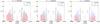 |
Fig. 14. Distributions of initial conditions (a0, i0) of surviving orbits after 1 Gyr evolution. The blue points are the 986 selected orbits without the Yarkovsky effect. The green points and red crosses indicate the survivors with Yarkovsky effect in retrograde and prograde rotation, respectively. From left to right panels, the absolute value of semi-major axis drift rates is 0.8, 1.2, and 1.6 AU/Gyr, respectively. Several points around i = 30° are ignored for a better vision. |
Wang & Hou (2017) proved that the libration amplitude of the semi-major axis in the 1:1 MMR undergoes remarkable variation when the Yarkovsky effect works. For prograde rotators, the amplitudes decrease with time while for retrograde rotators, the contrary is the case. As an example, we show in Fig. 15 the variations of semi-major axes of two Earth Trojans with the same initial orbital conditions but the opposite spinning direction and thus the opposite Yarkovsky effect. Clearly, the Earth Trojan in prograde rotation (γ = 0° thus  ) gets closer and closer to the libration centre of a ≈ 1 AU as time goes by. Once it crosses inward of the boundary of the tadpole region, the instability caused by the secular resonances and frequency drift as described in Sect. 4 may destabilize its orbit. Hence the closer the orbit is to the central area, the more likely it is to lose its stability. The instability in the central part of the 1:1 MMR leaves no country for Earth Trojans to hide. The same theory works for the retrograde rotators as well. The instability around the outer edge of the stability region eliminates the orbits in expansion of the semi-major axis.
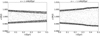 |
Fig. 15. Time evolution of the semi-major axis for one selected orbit whose lifespan is longer than 1 Gyr. The left panel is for a drift rate of 1.6 AU/Gyr corresponding to prograde rotation while the right panel for an opposite drift due to retrograde rotation. |
On the average the 986 selected orbits on the (a0, i0) plane are further towards the inner instability boundary than they are to the outer instability boundary (see Fig. 14). Therefore, it is easier for these orbits to approach the outer than the inner boundary under the semi-major axis drifts of the same rate but with opposite directions. In other words, the Earth Trojans of retrograde rotation ( ) are relatively easier to be driven out of the stable region in the 1:1 MMR. This finally makes the asymmetry of the surviving ratio in Fig. 13. Since the libration amplitudes of semi-major axis in the 1:1 MMR must keep increasing or decreasing for any non-zero Yarkovsky effect, the surviving ratio tends to be 0 after a sufficiently long time.
Orbits initially outside the 1:1 MMR region may drift towards the resonance region with the help of the Yarkovsky effect. For inner orbits (a < 1 AU) in prograde rotation, they can approach and enter the resonance region owing to a positive drift rate. At the time they cross the boundary from left side as a increases, the Yarkovsky effect acts together with the resonance to reduce the libration amplitudes of the semi-major axes. Consequently, they are promoted to go through the resonance region. However, for any asteroids that initially reside in the outer region (a > 1 AU) in retrograde rotation, the Yarkovsky effect increases the libration amplitudes of the semi-major axes at the time the asteroids cross the boundary from the right side as a decreases; this prevents these objects from entering further into the 1:1 MMR. Therefore, the Yarkovsky effect provides an effective one-way shield, preventing asteroids in the outer region (a > 1 AU) from entering the 1:1 MMR by virtue of the drift of the semi-major axis. This makes a bias favouring in a supplement of Earth Trojans from the inner side of the Earth orbit. In other words, if Earth Trojans are supplemented mainly by wandering objects through migration with the help of the Yarkovsky effect, most of these asteroids should have prograde rotation.
6. Conclusions and discussion
In this paper we were motivated to locate the stability regions around the Earth triangular Lagrange points L4 and L5. Simulations show that there are no outstanding dynamical differences between the orbits around these two points. We implemented the SN as the stability indicator and portrayed a much detailed dynamical map on the initial plane (a0, i0). We found that no stable orbits appear in the areas above i0 = 37°. Two main stability regions disconnected from each other are sheltered from chaos. One of these locates at low inclinations (i0 ≲ 15°) while the other occupies moderate inclinations (24 ° ≲i0 ≲ 37°). The most stable orbits (SN < 100) reside below i0 ≈ 10° and most of them could survive the age of the solar system. The chaos is widely distributed both inside and outside the stability regions. Furthermore, they are spreading to erode the stability regions.
The Kozai mechanism takes place in a high inclination area (i ≳ 40°) for an exchange of eccentricities. The subsequent close encounters with planets scatter the Trojans away. Moreover, the overlap of the secular resonances involving ν2 and ν3, even ν7 and ν8 brings in chaos for high-inclined orbits. However, the apsidal secular resonance with Jupiter still helps hold a window around 50° for orbits surviving for ∼6 Myr. Uranus and Neptune could make some difference to the stability in a relative short timescale.
To further research the resonance mechanism, we implemented a frequency analysis method to determine the locations of the secular resonances. The ν3 and ν4 secular resonances are found to be responsible for the instability gap separating the low and moderate inclination areas. They (especially ν4) have a large resonance width and could destabilize the orbits nearby by exciting their eccentricities. Most orbits undergo a small variation in inclination (Δi ≤ 10°) during their life except those surrounding the ν14 nodal secular resonance (Δi ∼ 20°). The transition from libration to circulation of ΔΩ3 also varies the inclination for orbits with different i0.
Higher degree secular resonances, of which the representatives are plotted in the secular resonance maps, give rise to the fine structures in dynamical maps. The separatrices between the tadpole and horseshoe orbits at 1 ± 0.0028 AU divide the whole phase space into three regimes and the orbits around the separatrices lose their stabilities in a short time. We classify the high-degree secular resonances into three types: G-type involves the apsidal precession of the Trojans alone, S-type involves the nodal precession alone, and C-type indicates the combination of the apsidal and nodal precession of the Trojans. The tadpole regions in the centre are mainly under the governance of C-type and G-type secular resonances, while the horseshoe regions on both sides are sculpted by S-type resonances.
Tabachnik & Evans (2000) indicated that there could be several hundred of primordial terrestrial companions provided the width of the stability zone around the Earth is 0.005 AU. We find in this paper that under the influence of the frequency drift of the inner planets, tadpole orbits can hardly survive the age of the solar system as the resonances they are trapped in show strong sensitivity to the precession rates of the planets. The instabilities can cover most of the tadpole cloud where the orbits with the longest lifespan reside (blue areas in the dynamical map) in a time long enough. To the contrary, most horseshoe orbits could remain almost unaffected and thus we have a chance to find the primordial terrestrial companions on horseshoe orbits.
The Yarkovsky effect modifies the stabilities of Earth Trojans by inducing the long-term evolution of their semi-major axis. We obtain the expression of the surviving ratio numerically to describe how different magnitudes of the Yarkovsky effect, which depends on the obliquity of the spin axis and physical properties such as the size and spin rate, affect the stabilities of Earth Trojans. The surviving ratio displays an asymmetry in prograde and retrograde rotations. Driven by the Yarkovsky effect, asteroids outside the 1:1 mean motion resonance may enter the resonance region, but the Yarkovsky effect has opposite influences on the prograde and retrograde spinning asteroids. As a result, asteroids are much more likely to enter the Trojan region from the inner region (a < 1 AU) and they must be in prograde rotation.
Adopting the typical values of physical and thermal parameters (for example bulk density, surface density, thermal conductivity, specific heat capacity, and emissivity) and typical spin-size relation, we find the threshold value of cos2/3γ/R (γ and R are the obliquity and radius) for Earth Trojans to survive the Yarkovsky effect. Further taking a surviving ratio of 1% as the critical probability, we find that an Earth Trojan surviving for 1 Gyr must have a radius larger than 90 m (130 m) if it has an exactly prograde (retrograde) spin. For those surviving the solar system age (4.5 Gyr), the smallest radius is 278 m for prograde spin and 400 m for retrograde spin, respectively.
The OSIRIS-REx (Origins, Spectral Interpretation, Resource Identification, and Security-Regolith Explorer) spacecraft has been launched on 8 September 2016 to conduct an asteroid study and sample-return mission. From February 9 to February 20, 2017, the spacecraft was located near the Sun-Earth L4 point to survey the sky covering ∼125 deg2 for Earth Trojans. Cambioni et al. (2018) claimed that no Earth Trojans were detected from the obtained images and this sets an upper limit for the population of Earth Trojans around the L4 point. Making use of the sensitivity curve, Cambioni et al. (2018) estimated that there could be no more than 73 ± 22 Trojans around L4 of absolute magnitude H = 20.5.
Our calculations indicate that any Earth Trojans with spin axis perpendicular to the orbital plane and albedo 0.05 have to be brighter than H = 20.0 to survive the Yarkovsky effect for 4.5 Gyr. If an albedo 0.10 as 2010 TK7 is adopted, they must be brighter than H = 19.4. In this sense, the 2010 TK7 with H = 20.7 cannot be a primordial Earth Trojan. Actually it is just temporarily in the Trojan orbit (Connors et al. 2011; Dvorak et al. 2012). These estimations, together with the null detection by the OSIRIS-REx mission, lead us to believe that there is only a very small possibility that any primordial Earth Trojan may still exist.
The Yarkovsky effect is not strong enough to drive Earth Trojans out of the resonance within the age of the solar system if the obliquity approaches γ = 90°. Our calculations show that the primordial Earth Trojans of albedo 0.10 fainter than the detection limit H = 20.5 must have the obliquity limited in a narrow range of 67°–103°, which is unlikely to be common.
Because of the uncertainties of the physical and thermal parameters of asteroids, we cannot absolutely deny the possibility of some exceptional primordial Earth Trojans existing nowadays. And of course, asteroids in the temporary Earth Trojan orbits cannot be excluded.
Acknowledgments
We thank the anonymous referee for comments that helped us improve the manuscript. This work has been supported by the National Natural Science Foundation of China (NSFC, Grants No. 11473016, No. 11473015 & No. 11333002). R.Dvorak wants to acknowledge the support from the FWF project S11607/N16.
References
- Bottke, Jr., W. F., Vokrouhlický, D., Rubincam, D. P., & Nesvorný, D. 2006, Annu. Rev. Earth Planet. Sci., 34, 157 [NASA ADS] [CrossRef] [EDP Sciences] [Google Scholar]
- Brasser, R., & Lehto, H. J. 2002, MNRAS, 334, 241 [NASA ADS] [CrossRef] [Google Scholar]
- Brasser, R., Heggie, D. C., & Mikkola, S. 2004, Celestial Mech. Dyn. Astron., 88, 123 [NASA ADS] [CrossRef] [Google Scholar]
- Cambioni, S., Malhotra, R., Hergenrother, C. W., et al. 2018, Lunar Planet. Sci. Conf., 49, 1149 [NASA ADS] [Google Scholar]
- Carpino, M., Milani, A., & Nobili, A. M. 1987, A&A, 181, 182 [NASA ADS] [Google Scholar]
- Chambers, J. E. 1999, MNRAS, 304, 793 [NASA ADS] [CrossRef] [MathSciNet] [Google Scholar]
- Christou, A. A., & Asher, D. J. 2011, MNRAS, 414, 2965 [NASA ADS] [CrossRef] [Google Scholar]
- Connors, M., Wiegert, P., & Veillet, C. 2011, Nature, 475, 481 [NASA ADS] [CrossRef] [Google Scholar]
- Ćuk, M., Hamilton, D. P., & Holman, M. J. 2012, MNRAS, 426, 3051 [NASA ADS] [CrossRef] [Google Scholar]
- Dvorak, R., Lhotka, C., & Zhou, L. 2012, A&A, 541, A127 [NASA ADS] [CrossRef] [EDP Sciences] [Google Scholar]
- Giorgini, J. D., Yeomans, D. K., Chamberlin, A. B., et al. 1996, BAAS, 28, 25.04 [Google Scholar]
- Hanslmeier, A., & Dvorak, R. 1984, A&A, 132, 203 [NASA ADS] [Google Scholar]
- Kozai, Y. 1962, AJ, 67, 591 [Google Scholar]
- Laskar, J. 1989, Nature, 338, 237 [NASA ADS] [CrossRef] [Google Scholar]
- Laskar, J. 1990, Icarus, 88, 266 [NASA ADS] [CrossRef] [Google Scholar]
- Laskar, J. 1993a, Phys. D Nonlinear Phenom., 67, 257 [Google Scholar]
- Laskar, J. 1993b, Celestial Mech. Dyn. Astron., 56, 191 [NASA ADS] [CrossRef] [Google Scholar]
- Laskar, J., Froeschlé, C., & Celletti, A. 1992, Phys. D Nonlinear Phenom., 56, 253 [CrossRef] [Google Scholar]
- Lhotka, Ch., & Dvorak, R. 2006, in A New Determination of the Fundamental Frequencies in our Solar System, In Proceedings of the 4th Austrian-Hungarian Workshop on Trojans and Related Topics, ed. A. Süli, et al. (Publication of the Astronomy Department of the Eötvös), 18, 33 [Google Scholar]
- Li, J., Zhou, L.-Y., & Sun, Y.-S. 2006, Chin. J. Astron. Astrophys., 6, 588 [NASA ADS] [CrossRef] [Google Scholar]
- Lidov, M. L. 1962, Planet. Space Sci., 9, 719 [NASA ADS] [CrossRef] [Google Scholar]
- Lykawka, P. S., Horner, J., Jones, B. W., & Mukai, T. 2009, MNRAS, 398, 1715 [NASA ADS] [CrossRef] [Google Scholar]
- Lykawka, P. S., Horner, J., Jones, B. W., & Mukai, T. 2011, MNRAS, 412, 537 [NASA ADS] [CrossRef] [Google Scholar]
- Mainzer, A., Bauer, J., Grav, T., et al. 2011, ApJ, 731, 53 [NASA ADS] [CrossRef] [Google Scholar]
- Marzari, F., & Scholl, H. 2013, Celestial Mech. Dyn. Astron., 117, 91 [NASA ADS] [CrossRef] [Google Scholar]
- Michtchenko, T., & Ferraz-Mello, S. 1993, Celestial Mech. Dyn. Astron., 56, 121 [NASA ADS] [CrossRef] [Google Scholar]
- Michtchenko, T. A., & Ferraz-Mello, S. 1995, A&A, 303, 945 [NASA ADS] [Google Scholar]
- Michtchenko, T. A., Lazzaro, D., Ferraz-Mello, S., & Roig, F. 2002, Icarus, 158, 343 [NASA ADS] [CrossRef] [Google Scholar]
- Mikkola, S., & Innanen, K. A. 1990, AJ, 100, 290 [NASA ADS] [CrossRef] [Google Scholar]
- Mikkola, S., & Innanen, K. 1992, AJ, 104, 1641 [NASA ADS] [CrossRef] [Google Scholar]
- Morbidelli, A., Levison, H. F., Tsiganis, K., & Gomes, R. 2005, Nature, 435, 462 [NASA ADS] [CrossRef] [PubMed] [Google Scholar]
- Murray, C. D., & Dermott, S. F. 1999, Solar System Dynamics (Cambridge, UK: Cambridge University Press) [Google Scholar]
- Nesvorný, D., & Dones, L. 2002, Icarus, 160, 271 [NASA ADS] [CrossRef] [Google Scholar]
- Nesvorný, D., & Vokrouhlický, D. 2009, AJ, 137, 5003 [NASA ADS] [CrossRef] [Google Scholar]
- Nesvorný, D., Morbidelli, A., Vokrouhlický, D., Bottke, W. F., & Brož, M. 2002, Icarus, 157, 155 [NASA ADS] [CrossRef] [Google Scholar]
- Nobili, A. M., Milani, A., & Carpino, M. 1989, A&A, 210, 313 [NASA ADS] [Google Scholar]
- Opik, E. J. 1951, Proc. R. Irish Acad. Sect. A, 54, 165 [Google Scholar]
- Scholl, H., Marzari, F., & Tricarico, P. 2004, Lunar Planet. Sci. Conf., 35 [Google Scholar]
- Tabachnik, S. A., & Evans, N. W. 2000, MNRAS, 319, 63 [NASA ADS] [CrossRef] [Google Scholar]
- Vokrouhlický, D. 1999, A&A, 344, 362 [NASA ADS] [Google Scholar]
- Wang, X., & Hou, X. 2017, MNRAS, 471, 243 [NASA ADS] [CrossRef] [Google Scholar]
- Weissman, P. R., & Wetherill, G. W. 1974, AJ, 79, 404 [NASA ADS] [CrossRef] [Google Scholar]
- Wiegert, P., Innanen, K., & Mikkola, S. 2000, Icarus, 145, 33 [NASA ADS] [CrossRef] [Google Scholar]
- Wolf, M. 1907, Astron. Nachr., 174, 47 [NASA ADS] [CrossRef] [Google Scholar]
- Zhou, L.-Y., Dvorak, R., & Sun, Y.-S. 2009, MNRAS, 398, 1217 [NASA ADS] [CrossRef] [Google Scholar]
- Zhou, L.-Y., Dvorak, R., & Sun, Y.-S. 2011, MNRAS, 410, 1849 [NASA ADS] [Google Scholar]
All Tables
Mean values and standard deviations of a0 (in AU) and i0 (in degree) of the orbits selected for the numerical fitting for g and s, respectively in regions L, C, and R.
Coefficients of the best fits for the proper frequencies g and s (in 2π yr−1) in regions L, C, and R on the (a0, i0) plane.
Mean values () and amplitudes of the variations (Δν) of the fundamental secular frequencies in the inner solar system, except for Mercury, over 200 Myr.
Upper limits of absolute magnitudes (H) of Earth Trojans of various albedos (α) surviving for 1 Gyr and 4.5 Gyr.
All Figures
|
Fig. 1. Dynamical map around the L4 point on the (a0, i0) plane. The colour indicates the SN of cosσ, which is shown on a base-10 logarithmic scale for more details. The orbits that escape from the Earth co-orbital region (see text) during the integration time (12 Myr) are excluded. The dashed lines indicate the separatrices between the tadpole and horseshoe orbits (see text in Sect. 4.2), which divide the dynamical map into three regimes. The tadpole orbits reside in the central region (denoted by “C”) while the horseshoe orbits are found in the left (“L”) and right (“R”) regions. |
| In the text | |
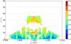 |
Fig. 2. Same as Fig. 1 but for L5 point. |
| In the text | |
|
Fig. 3. Dynamical maps for the possible stability window around i = 50° (Dvorak et al. 2012) on the (a0, i0) plane. The colour indicates the maximum eccentricity during the integration time. The four panels stand for the results derived from different models and integration times: Ve2Sa and integrated for 1 Myr (panel a), Ve2Sa for 12 Myr (panel b), Ve2Ne for 1 Myr (panel c), and Ve2Ne for 12 Myr (panel d). The stars in panelsa and c indicate the initial conditions for the orbits shown in Fig. 4. Magenta, black, and red stand for (a0, i0)=(0.9990, 48 ° ), (0.9990, 50 ° ) and (0.9982, 53 ° ), respectively. |
| In the text | |
|
Fig. 4. Orbital evolution of the fictitious Trojans indicated in Fig. 3 for the model Ve2Sa (red) and Ve2Ne (black). From left to right, the three panels corresponding to the magenta, black, and red stars are of the initial conditions of (a0, i0)=(0.9990, 48 ° ), (0.9990, 50 ° ), and (0.9982, 53 ° ). We illustrate the temporal evolution of e, Δϖ5, and i for both models, Δϖ7, Δϖ8, and ω for the model Ve2Ne only and Δϖ2, Δϖ3, ΔΩ2, and ΔΩ3 for the model Ve2Sa only. The vertical dashed lines in the bottom plots of each panel indicate the lifespans of the orbits being in the 1:1 MMR. |
| In the text | |
|
Fig. 5. Maximum eccentricity (in different colours) during orbital integrations of 12 Myr on the (a0, i0) plane. We show only for i0 ∈ [0 ° ,40 ° ] because there are no stable orbits with i0 > 37°. The black star stands for an orbit of (a0, i0)=(0.9999, 27 ° ) that is shown in Fig. 6. |
| In the text | |
|
Fig. 6. Orbital evolution of the fictitious Earth Trojan indicated in Fig. 5 with the initial condition of a0 = 0.9999 AU, i0 = 27°. From top to bottom panels: evolutions of the apsidal differences between the Trojan and Mars Δϖ4, the argument of the perihelion ω and eccentricity e. The red vertical dashed lines in the bottom panel indicate the lifespan of the orbit. |
| In the text | |
|
Fig. 7. Same as Fig. 5 but colours indicate the variation of inclinations. The black star stands for an orbit of (a0, i0)=(0.9958, 11 ° ) on the initial plane that is shown in Fig. 8. |
| In the text | |
|
Fig. 8. Evolutions of the nodal differences between the Trojan and Mars ΔΩ4 (top panel) and inclination i (bottom panel) of the fictitious Earth Trojan indicated in Fig. 7 with the initial condition of a0 = 0.9958 AU, i0 = 11°. |
| In the text | |
|
Fig. 9. Dynamical spectra of icosΩ (top panel) and ecosϖ (bottom panel) for orbits with initial inclinations i0 = 2°. The five most significant frequencies for each orbit are plotted against their initial semi-major axes. The frequencies with the largest amplitudes are labelled by red open circles while the second to the fifth are denoted by black open inverted triangles, squares, triangles, and diamonds, respectively. The blue dashed lines indicate the absolute values of the fundamental frequencies identified to be corresponding to forced frequencies. From top to bottom, they represent |s6|, |s3|, |s4|, 2g7 − s5, g4, g3 + s3 − s4, g2, and g5 respectively. We note that s3 and s4, (g3+s3−s4) and g4 are so close to each other that they are hardly distinguishable in the figure. Moreover, for a better vision, we just plot one-third of the data. |
| In the text | |
|
Fig. 10. Locations of main linear secular resonances for Trojans around the L4 point on the (a0, i0) plane. The resonances are labelled along the curves. |
| In the text | |
|
Fig. 11. Locations of the fourth-degree secular resonances for Trojans around the L4 point on the (a0, i0) plane. The resonances are labelled (see text for the meaning) along the curves. In consideration of the frequency drift of the inner planets, the dashed lines in the left panel delimit the possible locations of S4_A and G4_F (see Sect. 4.5). The black and red dashed lines represent the results derived from the data taken from Laskar (1990) and our integration, respectively. |
| In the text | |
 |
Fig. 12. Same as Fig. 11 but for sixth-degree secular resonances. |
| In the text | |
|
Fig. 13. Surviving ratio against evolution time for prograde spinning Trojans ( |
| In the text | |
|
Fig. 14. Distributions of initial conditions (a0, i0) of surviving orbits after 1 Gyr evolution. The blue points are the 986 selected orbits without the Yarkovsky effect. The green points and red crosses indicate the survivors with Yarkovsky effect in retrograde and prograde rotation, respectively. From left to right panels, the absolute value of semi-major axis drift rates is 0.8, 1.2, and 1.6 AU/Gyr, respectively. Several points around i = 30° are ignored for a better vision. |
| In the text | |
|
Fig. 15. Time evolution of the semi-major axis for one selected orbit whose lifespan is longer than 1 Gyr. The left panel is for a drift rate of 1.6 AU/Gyr corresponding to prograde rotation while the right panel for an opposite drift due to retrograde rotation. |
| In the text | |
Current usage metrics show cumulative count of Article Views (full-text article views including HTML views, PDF and ePub downloads, according to the available data) and Abstracts Views on Vision4Press platform.
Data correspond to usage on the plateform after 2015. The current usage metrics is available 48-96 hours after online publication and is updated daily on week days.
Initial download of the metrics may take a while.