| Issue |
A&A
Volume 698, June 2025
|
|
|---|---|---|
| Article Number | A42 | |
| Number of page(s) | 11 | |
| Section | Planets, planetary systems, and small bodies | |
| DOI | https://doi.org/10.1051/0004-6361/202553804 | |
| Published online | 27 May 2025 | |
New asteroid clusters and evidence of collisional fragmentation in the L5 Trojan cloud of Mars
1
Armagh Observatory and Planetarium,
College Hill,
Armagh
BT61 9DG,
UK
2
Department of Astronomy, University of Florida at Gainesville,
Gainesville,
FL
326112055,
USA
3
Division of Science, New York University Abu Dhabi,
Abu Dhabi,
UAE
4
Center for Astro, Particle and Planetary Physics (CAP 3), New York University Abu Dhabi,
UAE
5
Department of Physics and Astronomy, Queen’s University Belfast,
University Road, Belfast,
BT7 1NN,
Northern Ireland,
UK
6
SETI Institute, Mountain View,
CA
94043,
USA
7
INAF, Osservatorio Astrofisico di Arcetri,
50125
Firenze,
Italy
★ Corresponding author: This email address is being protected from spambots. You need JavaScript enabled to view it.
Received:
18
January
2025
Accepted:
8
April
2025
Abstract
Context. Trojan asteroids of Mars date from an early phase of Solar System evolution. The Mars Trojan (MT) distribution has been previously shown to be highly asymmetric and inhomogeneous. Remarkably, a single asteroid family associated with (5261) Eureka (H ∼ 16) at L5 contains all stable Trojans fainter than H = 18. A possible culprit is the action of thermal radiation forces on the orbits and rotation states of these small asteroids.
Aims. Using a larger MT sample than previously available, we took a fresh look at this population to re-evaluate these earlier conclusions. We also searched for additional features diagnostic of MT evolutionary history and of the Eureka family in particular.
Methods. We performed harmonic analysis on numerical time series of the osculating elements to compile a new proper element catalogue comprising 16 L5 and 1 L4 MT asteroids. We then combined sample variance analysis with statistical hypothesis testing to identify clusters in the distribution of orbits and assess their significance.
Results. We identify two small clusterings significant at 95% confidence of three H=20−21 asteroids each and investigate their likely origin. One of the clusters is probably the result of rotational breakup of a Eureka family asteroid ∼108 yr ago. The significantly higher tadpole libration width of asteroids in the other cluster is more consistent with an origin as impact ejecta from Eureka itself on a timescale comparable to the ∼1 gigayear age of its family. We further confirm the previously reported correlations in Eureka family orbital distribution attributed to the long-term action of radiation-driven forces and torques on the asteroids.
Key words: methods: numerical / methods: statistical / minor planets, asteroids: general / planets and satellites: individual: Mars
© The Authors 2025
 Open Access article, published by EDP Sciences, under the terms of the Creative Commons Attribution License (https://creativecommons.org/licenses/by/4.0), which permits unrestricted use, distribution, and reproduction in any medium, provided the original work is properly cited.
This article is published in open access under the Subscribe to Open model. This email address is being protected from spambots. You need JavaScript enabled to view it. to support open access publication.
1 Introduction
All major planets in the Solar System except Mercury feature asteroidal companions in the so-called tadpole or Trojan configuration, where a particle is confined to the vicinity of the Lagrangian triangular equilibrium locations that lead or trail the planet by 60∘ (Murray & Dermott 1999; Pan & Gallardo 2025). Numerical simulations demonstrate the transient nature of many of these Trojans and, by implication, their likely origin as dynamically unstable planet-crossing small bodies (Christou 2000; Morais & Morbidelli 2002; Connors et al. 2004).
Trojans of Jupiter, Neptune, and Mars have gigayear dynamical lifetimes and likely date from events early in Solar System history (Levison et al. 1997; Scholl et al. 2005; Lykawka & Horner 2010) with Mars featuring the only dynamically long-lived Trojans among terrestrial planets. Unlike Main Belt asteroids, the Mars Trojans (MTs hereafter) experience a relatively benign collisional environment while their proximity to the Sun and long dynamical lifetime make them a useful proving ground for models of asteroid orbital-rotational evolution by radiation forces (Rivkin et al. 2003; Ćuk et al. 2015; Christou et al. 2017).
Their small sizes notwithstanding (≤2 km; Trilling et al. 2007), MTs exhibit some unique features: a marked asymmetry favouring L5 vs. L4 residents (de la Fuente Marcos & de la Fuente Marcos 2013; Christou 2013); a strong orbital concentration near (5261) Eureka, suggesting that most L5 Trojans are products of YORP-induced rotational spin-up and breakup (‘YORPlets’; Christou et al. 2017); and the olivine-dominated composition of this Eureka family (Borisov et al. 2017; Polishook et al. 2017), one of only two known to exist (Galinier et al. 2024). Available compositional clues and dynamical models argue equivocally for either an asteroidal or a Martian origin for MTs (Polishook et al. 2017; Wargnier et al. 2025). Their continued study helps determine the nature of the link – if any – between MTs and the Martian system and our understanding of the early evolution of Mars by implication.
The Minor Planet Center website1 lists 18 MT asteroids, of which all but four have been confirmed as stable residents by numerical integration of the orbit (Scholl et al. 2005; Christou 2013; de la Fuente Marcos & de la Fuente Marcos 2013; Ćuk et al. 2015; Christou et al. 2020; de la Fuente Marcos & de la Fuente Marcos 2021). Of the two exceptions, 2023 FW14 is the second L4 Trojan of Mars to be discovered (de la Fuente Marcos et al. 2024). Its short, ∼ 107 yr dynamical lifetime points to a likely origin in the Mars-crosser population. The other asteroid, 2018 FM29, was discovered in 2018 and observed again in 2020, 2022, and 2024. The orbital semimajor axis uncertainty of this asteroid is now several orders of magnitude smaller than the radial width of the MT region (see Sect. 2.2) and we confirmed by numerical integration its status as a stable resident at L5. The recovery of single-opposition asteroids 2015 TL144 and 2016 AA165 in 2022 and 2024 respectively place them firmly within the Trojan clouds of Mars and we have similarly confirmed their stability with numerical integration of the orbits. Inclusion of the new Trojans raises the tally of MTs to 18 and of L5 residents in particular to 16.
Proper elements of gigayear-stable MT asteroids.
Using the methods described in the following Section of the paper, we calculated proper elements – libration width L, eccentricity eP and inclination IP – (Table 1) from the latest osculating elements of the objects available through the AstDys2 online service (Knežević & Milani 2012). Their distribution, shown in Fig. 1, exhibits several interesting features. Ćuk et al. (2015) note a strong correlation between libration width and inclination among Eureka family asteroids, showing it to be a consequence of the solar-thermal Yarkovsky effect (Bottke et al. 2006). We emphasise it is that correlation, rather than the direct detection of Yarkovsky acceleration in the orbital motion achieved recently for the near-Earth asteroids (e.g. Greenberg et al. 2020), that supports a Yarkovsky-dominated orbital evolution for MTs. Ćuk et al. further note that the asymmetric orbital distribution of family Trojans with respect to Eureka is compatible with a non-gravitational acceleration acting against the direction of motion. This might arise if bi-directional diurnal Yarkovsky is suppressed relative to the strictly dissipative seasonal variant through the coupling of spin and shape evolution (Rubincam 2000; Vokrouhlický & Čapek 2002; Čapek & Vokrouhlický 2004; Statler 2009; Cotto-Figueroa et al. 2015; Ćuk et al. 2015). Secondly, the new MTs have similar eccentricity and inclination to the Eureka family but much higher libration width. Their orbits are in fact similar to that of 2009 SE, an L5 Trojan that might be unrelated to Eureka (de la Fuente Marcos & de la Fuente Marcos 2021).
The availability of a larger MT sample than was available in earlier works motivates a fresh look at their orbital distribution using tools from dynamical systems and from statistical analysis. The present study uncovers evidence for a more complex evolutionary history of this population than recognised previously, including secondary rotational breakup of YORPlet asteroids and a role for collisions as a competing process for MT population evolution alongside thermal-rotational effects. In the next Section we expose the methods used to compile a new catalogue of MT proper elements, extract interesting features from it, and evaluate their statistical significance. Results are described in Sect. 3 while in Sect. 4 we examine origin scenarios for the new clusters. In Sect. 5 we present our conclusions.
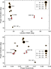 |
Fig. 1 Distribution of L5 MTs in libration width (L) vs. inclination (IP) space (top) and eccentricity eP vs. inclination IP (bottom). Red points correspond to new asteroid clusters identified in this work. Plotted errors correspond to 2σ formal uncertainties and are smaller than the symbol size for the libration width L. |
2 Methods
2.1 Confirming the stability of MTs 2009 SE, 2015 TL144, 2016 AA165 and 2018 FM29
To determine the long-term stability of candidate Trojans, we generated 50 dynamical clones of each asteroid from the state covariance at epoch MJD 60 600.0 available through AstDys using the method of Duddy et al. (2012). The clones plus the nominal orbit were then numerically integrated for 109 yr with the MERCURY package (Chambers 1999) under the gravity of the eight major planets and an integration time step of 4d. For all clones of each asteroid, the critical angle lr=λ − λMars remained in libration around −60∘ until the end of the integration, indicating dynamical lifetimes comparable to the Solar System age. Examples of individual clone orbital evolution are shown in Fig. 2 where we also included 2009 SE. In the case of 2015 TL144 we observe libration width variations of 5∘−10∘ over timescales of 108 yr. We observe such variations in most clones of the asteroid and attribute them to the proximity of the orbit to the chaotic region surrounding the tadpole-horseshoe separatrix at a libration width of ∼ 156∘ (Morais 1999). Otherwise, the clone integrations imply similar dynamical stability to the other Trojans.
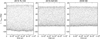 |
Fig. 2 Critical angle evolution over 109 yr for dynamical clones of selected MT asteroids. |
2.2 Modelling tadpole libration of MTs
In the context of the circular restricted Sun-planet-asteroid problem, the evolution of the guiding centre ar(lr) in the vicinity of the planetary orbit (|ar| = |a−aP| ≪ 1) is described by the integral (Namouni et al. 1999)
 (1)
(1)
 (2)
(2)
where C is a constant, r and rP are the heliocentric position vectors of the asteroid and planet respectively, lr = λ−λP and distances are in units of aP. As S has a minimum Smin ≃ 1/2 at lr≃± π/3, Eq. (1) can be written as
 (3)
(3)
where ΔS = S − Smin and  = C − (8μ/3) Smin. The radial width a0 for tadpole libration was obtained by evaluating Eq. (3) at the turning points for 0<ΔS < 1. For e ∼ 0, I ∼ 0∘ and Δ S = 1 we obtain the classical result (Yoder et al. 1983; Murray & Dermott 1999; Morais 1999, 2001) that
 (4)
(4)
For the case of Mars, we used μ ∼ 3.2 × 10⁻⁷, aP ∼ 1.524 au and found
 (5)
(5)
At large libration amplitude, the motion of the guiding centre around the equilibrium point is strongly asymmetric (Érdi 1988; Milani 1994). For this reason, we chose to parameterise the resonant state of the asteroid orbit by the full width of lr libration rather than the libration amplitude D (Milani 1993; Ćuk et al. 2015). We refer to this width as L so that, for small libration amplitude (S ≳ Smin), L ≃ 2 D. We also chose d̄ = a0/a0, max = Δ S as the action-like quantity, obtained by numerical evaluation of Eq. (3) at ar = 0 with ω = 0∘, e = 0, and I = 0∘. Our approach in determining the resonant elements is similar to that of Vokrouhlický et al. (2024) for the Jupiter Trojans. We report proper element estimates for the MTs in Table 1 while pointing out that the moderate inclination of MTs modifies the effective potential with respect to the planar case (Fig. 3). The principal effect of the change is a planetward displacement of the turning point of the tadpole by up to ∼ 4∘ and an increase in L by a similar amount, manifesting as a fixed offset in the libration widths of the clusters investigated in Sect. 3.2. Including the correction does not alter the orbital dispersion of MT families (Sects. 3.1 and 3.2) and we chose not to include it in our computation of L to maintain consistency with existing proper element catalogues (e.g. Vokrouhlický et al. 2024).
2.3 Proper element estimation
We calculated the proper eccentricity and inclination by carrying out a ∼7.3 × 10⁵ yr integration of the nominal orbit as described in Sect. 2.1 sampled every 128d. The complex quantities z=e exp i ϖ and ζ = I exp iΩ formed from the output were then fitted to Fourier series of the form
 (6)
(6)
using the Frequency-Modified Fourier Transform algorithm (FMFT; Sidlichovský & Nesvorný 1997). The coefficients Ai and Bi in Eq. (6) are complex quantities. The frequencies vi, μi with i ≠ 0 are linear combinations of the fundamental Solar System secular eigenmodes (Laskar et al. 2004) while ν0 and μ0 are the free precession eigenmodes of the asteroid and  . Proper elements were recovered from the fit as eP=|A0| and IP=|B0|.
For the libration width L we adopted the average of the difference between the maximum and minimum value of lr within a 120-sample window applied to the numerical time series. An example of this procedure is shown in Fig. 4. Finally, we obtained d̄ from L by evaluating Eq. (3) for a circular, planar orbit as described in the previous Section.
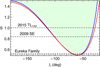 |
Fig. 3 Profiles of the effective potential (Eq. (2)) for tadpole-type libration (green) evaluated with I = 0∘ (blue curve) and I = 20∘ (red curve) to highlight the effect of orbital inclination on libration width. |
2.4 Statistical tests of cluster significance
To establish that any particular asteroid grouping represents a real association, we used Monte-Carlo simulations to form the distribution of an appropriate test statistic. That distribution was then compared against the value of the statistic for the candidate cluster to estimate the probability – or p-value – that the claimed cluster is a chance arrangement between unrelated objects. Two different statistical functions were used, one based on the Minimum-volume Enclosing Sphere (MES) and the other on the Cluster Index (CI).
Given a set of m points in a multi-dimensional Euclidean space, the MES of that set is defined by the property that
 (7)
(7)
where P(x0, r0) is the sphere with centre x0 and radius r0 while V(P) is the sphere volume, used here as a measure of compactness for a given m-subset of M proper orbits.
On each MC trial, we generated a synthetic set of M random points from some reference distribution representing the null hypothesis of uniformity. We then calculated the MES volume V(PMES) for every possible m-subset of points and compared it with the MES volume for the candidate asteroid cluster V(PMES,c)=Vc, recording a ‘hit’ when the condition minj V(Pj) < η Vc is satisfied, where j runs through the set of subsets. The quantity
 (8)
(8)
then estimates the probability that a cluster as compact as our candidate cluster could have arisen by chance. We introduced the η factor as a convenient way to incorporate the different sources of uncertainty in MES volume calculation. In this paper, we used η = 3.0 as a compromise between applying an overly strict criterion and the risk of underestimating Vc due to the statistical uncertainty in the proper orbits.
The Cluster Index (Liu et al. 2008; Huang et al. 2015, see also Markwardt et al. 2023) is defined as
 (9)
(9)
where x̄(j) is the mean for the j-th out of N clusters within a sample of M points and x̄ is the overall sample mean. A CI value ≪ 1 implies a strongly-clustered set. The synthetic set of orbits in each Monte Carlo trial was split into N=2 clusters (of size M1 and M2 respectively) by the kmeans unsupervised clustering search algorithm (MacQueen 1967) implemented via the FindClusters function in Mathematica v12.0 (Wolfram 2003). The procedure initially assigns random centroids to the k clusters with each point subsequently assigned to its nearest centroid. The CI values for the randomly-generated sets form the cumulative distribution function to be compared with the CI value for the candidate asteroid cluster. The p-value was then estimated in a manner analogous to the MES method, that is
 (10)
(10)
Kmeans requires the number of clusters as input. Here we used the Elbow method (Thorndike 1953) to heuristically determine the optimum cluster number for our sample by evaluating the numerator in Eq. (9) as a function of k. This is the Within-Cluster Sum of Squares (WCSS; MacQueen 1967) with the property that it vanishes as k → M. The evaluation at k=2 (Fig. 5) corresponds to an ‘elbow’ – the largest change between consecutive values as well as the largest change between consecutive changes – as the optimum cluster number in this case. We present a full listing of our statistical tests and their outcomes in Table 2.
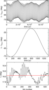 |
Fig. 4 Example of libration width estimation for MT 2011 SC191 from the numerical simulations. Top: evolution of the critical angle lr. Middle: variation of lr over one boxcar width of 120 samples or ∼ 1350 yr. Bottom: variation of the L estimate over all boxcar windows with the average value (red dashed line) reported in Table 1. |
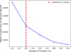 |
Fig. 5 WCSS evaluation as a function of the cluster number k in kmeans. The elbow (vertical dashed line) identifies the optimum value k = 2. |
3 Results
3.1 Eureka family structure and the role of Yarkovsky
A notable feature of the Eureka family is a strong anti-correlation between libration width and proper inclination (Fig. 1, top panel). We attribute this to Yarkovsky-driven coupled evolution of L and sin I, while the evolution of the eccentricity is dominated by random diffusive growth (Ćuk et al. 2015; Christou et al. 2020). Numerical models of orbital evolution via either mode suggest an approximate family age of 1 Gyr when compared to the observed orbital dispersion (Ćuk et al. 2015). Here we revisit these conclusions with the benefit of a larger sample of family asteroids and improved orbit determination due to longer observational arcs. The shape and orientation of the family may be computed from the sample covariance matrix (Johnson & Wichern 2007)
 (11)
where x = {[d̄i, ei, sin Ii]}i=1⋯s M is a 3 × M matrix with rows the proper elements for the N family members, x̄ is the sample mean and the superscript ‘T’ indicates the transpose. The eigenvalues and eigenvectors of Σ, reported in Table A.1 define the shape and orientation of Gaussian elliptical iso-contours as shown in Fig. 6. The coordinate frame defined by the ellipse principal axes amounts to an anticlockwise rotation by an angle θ = 163.7∘ from the positive d̄ axis. A statistical measure of association between d̄ and sin I is the Pearson correlation coefficient
(11)
where x = {[d̄i, ei, sin Ii]}i=1⋯s M is a 3 × M matrix with rows the proper elements for the N family members, x̄ is the sample mean and the superscript ‘T’ indicates the transpose. The eigenvalues and eigenvectors of Σ, reported in Table A.1 define the shape and orientation of Gaussian elliptical iso-contours as shown in Fig. 6. The coordinate frame defined by the ellipse principal axes amounts to an anticlockwise rotation by an angle θ = 163.7∘ from the positive d̄ axis. A statistical measure of association between d̄ and sin I is the Pearson correlation coefficient
 (12)
(12)
with values between +1 or −1 (Johnson & Wichern 2007). The two extremes correspond to points lying along a line. For the sample of M = 12 Eureka family members we find
 (13)
(13)
that is a strong inverse association between d̄ and sin I. Using only the seven asteroids considered in Ćuk et al. (2015) we obtain the slightly higher negative correlation of −0.971. In contrast, we find no evidence of correlation of either of those elements with e(|n23|, |n12| <0.05).
These results reinforce the conclusions of Ćuk et al. (2015) on the controlling influence of non-gravitational forces in the orbital distribution of MTs. Moreover, all of the five additional Trojans in this study (blue points in Fig. 6) are located either near Eureka or to higher d̄ and lower sin I. Therefore, the asymmetric distribution of family Trojans relative to Eureka attributed to the dominance of the seasonal Yarkovsky effect in the 2015 study is also confirmed for our 1.7 × larger sample.
Agglomerative hierarchical clustering (Ward 1963) was applied in de la Fuente Marcos & de la Fuente Marcos (2021) to a set of 44 Mars co-orbitals in the space of Tisserand constant (Tisserand 1896) vs. the critical angle lr. Those authors find that all family members known at that time clustered near Eureka. We applied the same procedure on the Eureka family but now in the space of proper elements with values listed in Table 1, using the same s/w implementation of the algorithm as those authors from the SciPy Python library (Virtanen & et al 2020) through the linkage and dendrogram functions and with a distance function of the form
 (14)
(14)
Here the subscript ‘PB’ represents the chosen parent body and the first term represents the quantity (a−aPB)/aPB for our chosen set of variables. We used the following three choices for the vector (A, B, C):(5/4, 2, 2), (1/4, 2, 2) and (1, 1, 1). The last choice corresponds to the standard Euclidean distance used in de la Fuente Marcos & de la Fuente Marcos, while the other two choices correspond to the traditional Hierarchical Clustering Method (HCM) as applied to Main-Belt asteroids (Zappalà et al. 1990, 1994) and to the Jupiter Trojans (Milani 1993) when single linkage is used. In all our runs, the clustering procedure was started from (5261) Eureka.
Significance test results for the MT clusters as described in the text.
Figure 7 shows the dendrogram output for both single and complete linkage. In the single linkage runs, asteroid 2011 SC191 was always separated from the rest of the group, probably reflecting its status as the family member with the lowest inclination and highest libration width (Fig. 6). The similarity of dendrograms produced by the Zappalà and Milani metrics suggests a relatively minor contribution from the semimajor axis term in Eq. (14). A compact grouping identified in all cases is composed of 2011 SP189, 2018 EC4 and 2018 FM29 with δ [L, e, I]=0.38∘ ± 0.21, 0.0017 ± 0.0021, 0.18∘ ± 0.14∘ (errors reported at 2-σ significance). Hereafter we refer to this grouping as the 2018 EC4 cluster after its brightest member and investigate it more closely in the next section.
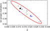 |
Fig. 6 Orbital distribution of Eureka family asteroids. Grey points represent objects considered in Ćuk et al. (2015) while blue points are new Trojans. The black point is (5261) Eureka. The red ellipse demarcates a 95% confidence region from the variance analysis and the “+” sign marks the mean family orbit. |
3.2 New MT clusters
To investigate the statistical significance of the 2018 EC4 cluster we applied the MES compactness criterion (Sect. 2.4) with a Gaussian null distribution defined from the sample of M = 12 Eureka family asteroids. The cumulative distribution of MES volumes for 1000 Monte Carlo trials and for all possible m = 3 subsets is shown in Fig. 8, top panel. We find a ∼4% probability that a grouping more compact than these three asteroids could have occurred by chance within the Eureka family. If we include nearby asteroid (311999) to this group and repeat the procedure, we find that this larger grouping is no longer significant (p-value >0.5). We therefore conclude that the EC4 cluster is the largest statistically significant sub-grouping of family asteroids under the current observational completeness of the family. We return to the relation between this cluster and (311999) in Sect. 4.
Turning now to Trojans outside of the Eureka family, we observe that the libration widths of two of the new stable Trojans highlighted in Table 1 are much higher than any Eureka family member but similar to that of 2009 SE, with the proper orbit of 2016 AA165 in particular being almost identical to that of 2009 SE (δ [L, e, I] = 0.36∘ ± 0.96∘, 0.0002 ± 0.0021, 0.23∘ ± 0.14). Asteroid 2015 TL144 has the highest libration width of any stable MT to-date, including (121514) at L4 (Table 1), but otherwise its eccentricity and inclination are similar to those of the other two asteroids (δ [e, I] = 0.0027 ± 0.0021, 0.34∘ ± 0.14∘). The strongly elongated shape of this orbital grouping (σd̄ ≫ σe, σsin I) renders the MES approach unsuitable and we resort to the CI-based approach to assess its statistical significance as a cluster of related asteroids.
Application of the kmeans algorithm with k = 2 separated the population of M1 + M2 = 15 L5 asteroids into the candidate cluster and the Eureka family with a CI value >99.9% significant against the null hypothesis (Table 2). To test the robustness of the result, we replaced the Gaussian d̄ variate with a uniform variate drawn between 0 and 0.6 and repeated the procedure. We then substituted the full Eureka family with only the 3 brightest family members to force size parity between the two clusters. We again find that kmeans separates the clusters with >95% significance (Fig. 8, middle panel). Identification of this grouping as a separate cluster is therefore robust and these small asteroids must be related in some way. For the remainder of the paper, we identify this cluster by its brightest member, 2009 SE.
In additional clustering experiments, we found that reapplication of kmeans but now with k=3 again separates out the 2009 SE cluster and additionally a Trojan pair formed by the Eureka family members with highest eP in Table 1. Applying instead the DBSCAN clustering algorithm (Ester et al. 1996) yielded the same result except that the new cluster was composed of the three highest eP Trojans. The large eccentricity and inclination spread among members of this cluster (δ eP ≃ 0.023, δ IP ≃ 2.6∘) however indicates that its identification was spurious and we do not consider it further here.
We further investigated the very close pair 2016 AA165 − 2009 SE by using the MES approach. As for the full cluster (Table 2), its statistical significance depends on the initial sample size M. For M=15 we obtained a significance of 91%, however this assumption ignores the strong statistical association between Eureka family asteroids. Reducing the sample size to M=6 (Fig. 8, bottom panel) and then M=4 as done previously increased significance to 96 and 99.5% respectively, on a par with our earlier conclusions for either cluster.
As a final note in this Section, we point out that the asteroid sizes in these clusters are comparable to – though at the lower end of – members of identified pairs and clusters in the Main Belt (Vokrouhlický & Nesvorný 2008; Pravec et al. 2010, 2018). MB clusters are recognised by virtue of remarkably similar osculating orbits between members. The new Trojan clusters do not show this degree of similarity (Table 3) and are likely older than their MB counterparts (see next section). We postulate that they remained compact and identifiable by virtue of similar proper orbits owing, on one hand, to the overall sparsity of MT asteroids and, on the other, their spatial confinement 60∘ ahead or behind Mars which mitigates differential orbital evolution by inverse-distance perturbations from the other planets (Christou 2013).
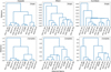 |
Fig. 7 Dendrograms from agglomerative clustering analysis of the Eureka family with different orbital distance choices (Eq. (14)) and adopting either single or complete linkage. |
Osculating orbital elements of candidate cluster MT asteroids at epoch JD 2460600.5
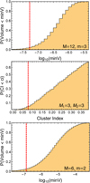 |
Fig. 8 Statistical tests for candidate MT clusters. From top to bottom: MES volume distribution versus the test statistic value (red line) for the 2018 EC4 cluster; CI distribution versus the test statistic value for the 2009 SE cluster; and MES volume distribution versus the test statistic value for the 2009 SE – 2016 AA165 pair. |
4 Discussion: cluster origin scenarios
4.1 2018 EC4 cluster: A potential product of cascade disruption?
Asteroids in both new groups occupy a relatively narrow range in H implying similar-sized objects. We can estimate asteroid size through the expression
 (15)
(15)
if the geometric albedo pv is known (Bowell et al. 1989). Here we assumed pV=0.2 similar to other Eureka family asteroids (Christou 2013). For the EC4 cluster we obtained nominal diameter estimates of 276 m (2018 EC4), 191 m (2011 SP189) and 175 m (2018 FM29), yielding same-density mass ratios in the range 0.25–0.77, generally high for products of YORP-induced rotational fission (mass ratio ∼0.2; Pravec et al. 2010, 2018).
Alternatively, the parent body of this cluster is another Eureka family asteroid. The nearest family member is (311999) (Fig. 1) with D ∼ 0.7 km. A genetic relationship with this asteroid is more compatible with the rotational fission mechanism. Even if the group separated from (311999) as a single object, the inferred mass ratio of 0.094 fits comfortably within the range predicted by fission theory. A relatively young age for this cluster as implied by its apparent compactness is also consistent with separation from (311999). This asteroid is likely a Eureka YORPlet itself, therefore a link to the cluster implies an ongoing process of cascade disruption of the Eureka progenitor, similar to that invoked for some Main Belt clusters (Fatka et al. 2020).
By comparing the orbital distribution of numerically propagated test particles under the Yarkovsky effect to the observed distribution of Trojans, Ćuk et al. (2015) obtain an approximate upper limit on the family age of 1 Gyr, corresponding to the separation event responsible for 2011 SC191 (point at extreme bottom right in Fig. 6). We make use of that result here to estimate the age of the EC4 cluster. We assumed that the separation distance s in d̄ − sin I space3 of the asteroid from the parent body after time tage is related to the separation rate ṡ by
 (16)
(16)
If the same inverse-linear size dependence holds for ṡ as for the semimajor axis drift ȧ in the absence of resonance, Eq. (16) becomes
 (17)
(17)
From the analysis in Sect. 3.1 we have sSC191 ≃ 0.0536. Adopting pV = 0.4 for Eureka family asteroids as in Ćuk et al., Eqs. (15) and (17) yield
 (18)
(18)
and, by applying Eq. (17) to (311999) and each of the EC4 cluster asteroids we obtain tage = 44−127 Myr. As the Yarkovsky drift rate depends on a number of unknown bulk and surface characteristics of the asteroid (Bottke et al. 2006), the size-corrected value obtained here may differ from that of 2011 SC191. An additional uncertainty factor of ∼2 arises from the statistical uncertainty of the computed proper elements (Table 1). However, even if the true separation ages are several times shorter than our estimated lower bound, this cluster appears to be significantly older than other previously identified clusters or pairs of small main-belt asteroids (≲ 4 Myr; Pravec et al. 2018, 2019).
4.2 2009 SE cluster as the outcome of collisional fragmentation
The similar eccentricity and inclination between this cluster and the Eureka family on one hand but much higher libration width on the other, could arise if this cluster is a remnant of an ejecta cloud from a past collision on an MT. Such ejecta would escape from the surface of a parent body of diameter D and bulk density ρ if vej > vesc where
 (19)
(19)
and G is the universal gravitational constant. The separation velocity of magnitude  for escaping fragments would cause differences between fragment and parent body orbits given by the Gauss equations (e.g. Nesvorný et al. 2006):
![Mathematical equation: $\delta a / a =\frac{2}{\mathrm{v}_{\text {circ}}\left(1-e^{2}\right)^{1 / 2}}\left[(1+e \cos f) \mathrm{v}_{t}+(e \sin f) \mathrm{v}_{r}\right]$](/articles/aa/full_html/2025/06/aa53804-25/aa53804-25-eq23.png) (20)
(20)
![Mathematical equation: $\delta e =\frac{\sqrt{1-e^{2}}}{\mathrm{v}_{\text {circ}}}\left[\frac{e+2 \cos f+e \cos ^{2} f}{1+e \cos f} \mathrm{v}_{t}+(\sin f) \mathrm{v}_{r}\right]$](/articles/aa/full_html/2025/06/aa53804-25/aa53804-25-eq24.png) (21)
(21)
 (22)
(22)
where the orbit elements are those of the parent asteroid,  is the heliocentric speed for a circular orbit of radius a while vt, vr and vw are the respective transverse, radial and out-of-plane components of vsep. For e∼0 and a = aP, Eqs. (4) and (20) give
 (23)
(23)
for the minimum velocity ‘kick’ needed to evict a small-amplitude (d̄∼0) MT. A kick of this magnitude would, at the same time, have a negligible effect on the other elements (δe, δI = O(10−3) from Eqs. (21) and (22)). Figure 9 shows the distribution of randomly-generated particles that separated from Eureka and (311999) with fixed separation speeds of 5, 20 and 200 m s−1. Their orbits were obtained from Eqs. (20)–(22) by sampling ω and f uniformly over the range 0-2π and for an isotropic separation direction. Values for the remaining elements were set to be those of the respective parent asteroids while L was calculated from δa using the method of Vokrouhlický et al. (2024).
We observe that a separation speed of 5 m s−1 from either (5261) or (311999) is sufficient to increase L to the values in the 2009 SE cluster (top panel). This scenario is compatible with separation from (311999) in particular, except that an additional mechanism is then required to increase e from 0.045 to ∼ 0.06 to match that of (311999) (bottom panel). Delivering such a change in fragment eccentricity from an impact on the asteroid requires a separation speed of 200 m s−1, much higher than typical fragment ejection speeds from collisional disruption of km-sized bodies (≤10 m s−1; Jutzi et al. 2010).
An additional factor to consider is the timing of the impact event and subsequent orbital evolution of the fragments. We have seen (Sect. 3.1 and Ćuk et al. 2015) that small MTs would gradually migrate to orbits with lower inclination and higher libration width due to the Yarkovsky effect. Low-speed ejection of the 2009 SE cluster asteroids from (5261) sometime in the past readily delivers the asteroids to their observed orbits without the need to invoke unusually high ejection speeds. Since the cluster’s proper inclination is significantly lower from Eureka, the time elapsed since the collision event would be comparable to the Eureka family age. Assuming a similar rate of orbital migration and working as in Sect. 4.1, we find tage ≃ 400 Myr.
The origin scenario we propose for this cluster is compatible with the one available model of the likely collisional history of the Trojans (Christou et al. 2017). The model gives about even odds that Eureka experienced no catastrophic disruption (Q ∼ Q* where Q is the impactor kinetic energy per unit target mass and Q* is an impactor- and target-dependent threshold; Housen & Holsapple 1990; Benz & Asphaug 1999) over the age of the Solar System. Impacts with Q < Q* should occur more frequently and we propose that at least one such event capable of imparting a speed of ∼ 5 m s−1 to fragments 1/10 the size of Eureka occurred within the last ∼1 Gyr of Solar System history.
Interestingly, this timeframe is also the expected collisional lifetime of D∼300m MTs such as 2009 SE and 2018 EC4 (Christou et al. 2017). The existence of either clusterings might therefore signify their relatively recent creation from progenitor bodies derived from Eureka, (311999) or both. In some cases the member separation epoch in young asteroid families may be constrained by backwards propagation of the orbits (Nesvorný et al. 2002; Carruba et al. 2018). We relegate such an exercise for the MT families to future work.
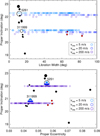 |
Fig. 9 Orbital distribution of 100 particles (blue open symbols) that separated from asteroids (5261) and (311999) (black open symbols) with different speeds. Particle sets are staggered by 0.1∘ in inclination for clarity. Red points correspond to members of the 2009 SE cluster. |
5 Conclusions
We identify three new faint (H=20−21) L5 MTs, raising the total number of trailing Trojan cloud residents to 16. Among the new finds is 2015 TL144 with the highest width of tadpole-type libration (∼ 83∘) among stable MTs.
The new Trojans have similar eccentricity and inclination to the previously identified Eureka family of MT asteroids (Christou 2013; de la Fuente Marcos & de la Fuente Marcos 2013). However, two of the objects have quite high libration width and may not be rotational fission products (‘YORPlets’) as suggested for Eureka family asteroids (Christou 2013; Ćuk et al. 2015; Christou et al. 2020). We propose instead that these objects, together with 2009 SE identified previously by de la Fuente Marcos & de la Fuente Marcos (2021), originated as collisional impact ejecta from a Eureka family asteroid with the most likely parent being (5261) Eureka itself. We also identify an additional statistically significant cluster of similarly faint Eureka family members that may have formed as YORPlets of asteroid (311999) sometime in the last 108 yr.
We revisit the significance of the correlation between libration amplitude and inclination attributed to Yarkovsky-driven orbital evolution (Ćuk et al. 2015) by calculating the Pearson correlation coefficient for the Eureka family asteroids. Our estimate of 94% implies a strong association between these two orbital properties. We further confirm the lack of Eureka-derived YORPlets with orbital evolution dominated by a positive Yarkovsky acceleration, consistent with the proposed dominance of the seasonal over the diurnal Yarkovsky effect over the ∼ 1 Gyr age of the family (Ćuk et al. 2015).
The decadal Legacy Survey of Space and Time (LSST; Jones et al. 2016) will discover and catalogue approximately 5 million main belt asteroids in addition to the ≳1 million currently known. Assuming similar discovery efficiency and a size distribution n (< D) ∝ D−0.45 for MTs (Christou et al. 2020), LSST should find ∼ 70 new MTs as faint as H=23 (D∼75 m for a geometric albedo of 0.2), allowing to test the conclusions of this paper by comparing the orbital distributions of those smaller asteroids and of existing MTs. The outcome of this exercise will have wider implications for the efficiency of diurnal vs. seasonal Yarkovsky and the relative roles of radiation forces vs. collisions for sub-km asteroids on timescales 107−109 yr. This is a regime where few observational constraints exist, yet extremely relevant to the important coupled problems of NEA/meteorite source regions and the migration routes of asteroid fragments to the Earth.
Acknowledgements
A.D.O. was supported by a grant of the Italian National Institute for Astrophysics for fundamental researches projects (INAF, act n. 38/2023). Work by A.H. was supported by the Science and Technology Facilities Council (STFC). We would like to thank the High Performance Computing Resources team at New York University Abu Dhabi and especially Jorge Naranjo for helping us with our numerical simulations. Insightful comments by the anonymous reviewer significantly improved the manuscript. Astronomical research at the Armagh Observatory & Planetarium is grant-aided by the Northern Ireland Department for Communities (DfC).
Appendix A Statistical analysis of Eureka family proper orbits
Table A.1 shows the covariance and correlation of the sample of proper orbits in Table 1 as well as the covariance matrix eigenvalues and eigenvectors used in Sect. 3.1.
Proper element sample moments and covariance spectral decomposition for the 12 Eureka family asteroids.
Appendix B Uncertainty modelling of MT proper element estimates
Formal uncertainties reported in Table 1 were calculated as
 (B.1)
(B.1)
where x = L, eP or IP, the first term under the square root refers to the orbit uncertainty and the second to the fitting model. Estimates of σx, o and σx, m for the MTs are shown in Table B.1.
For the libration width, we adopted as model uncertainty σL, m the 2-σ dispersion of the 120-sample estimates obtained from the numerical time series (Sect. 2.3). To calculate the error introduced by the filtering procedure in estimating σe, m and σI, m, we applied FMFT to selected MTs and for different Fourier polynomial order n (2, 5, 10, 15 and 20). Fig. B.1 shows these estimates shifted vertically to match the value at n = 10. Consequently, we adopted the values 0.0015 and 0.1∘ containing 95% of eP and IP estimates as respective model errors for all MTs.
Proper element uncertainties of MT asteroids.
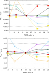 |
Fig. B.1 Estimates of proper eccentricity (top) and inclination (bottom) of MTs obtained by applying FMFT for different Fourier polynomial order. Displayed values are referenced to the case n=10. Dashed horizontal lines show the adopted formal uncertainties in this work. |
To estimate the uncertainty arising from the finite knowledge of the orbit, the asteroids were first ranked according to the semimajor axis uncertainty σa, as the coorbital state is most sensitive to this element. This information was obtained from the state covariance for epoch JD2460600.5 from AstDys. These values ranged between ∼2 × 10⁻⁹ au (5261) to ∼2 × 10⁻⁶ au (2009 SE). Each asteroid was then assigned to one of three bins demarcated by the values σa = 5 × 10⁻⁷ au and σa = 5 × 10⁻⁸ au. We selected one representative for each bin, calculated proper elements for 20 dynamical clones of each and adopted 95% confidence intervals from the 20-sample statistics as our estimates of σx, 0 for all asteroids in the respective bins. The bin representative asteroids in order of increasing σa were (5261), 2009 SE and 2015 TL144.
References
- Benz, W., & Asphaug, E., 1999, Icarus, 142, 5 [NASA ADS] [CrossRef] [Google Scholar]
- Borisov, G. B., Christou, A. A., Bagnulo, S., et al. 2017, MNRAS, 466, 489 [NASA ADS] [CrossRef] [Google Scholar]
- Bottke, W. F., Vokrouhlický, D., Rubincam, D. P., & Nesvorný, D., 2006, Ann. Rev. Earth Planet. Sci., 34, 157 [Google Scholar]
- Bowell, E., Hapke, B., Domingue, D., et al. 1989, in Asteroids II (Tucson: University of Arizona Press, Tucson), 524 [Google Scholar]
- Čapek, D., & Vokrouhlický, D., 2004, Icarus, 172, 526 [Google Scholar]
- Carruba, V., De Oliveira, E. R., Rodrigues, B., & Requena, I., 2018, MNRAS, 479, 4815 [NASA ADS] [CrossRef] [Google Scholar]
- Chambers, J. E., 1999, MNRAS, 304, 793 [Google Scholar]
- Christou, A. A., 2000, Icarus, 144, 1 [NASA ADS] [CrossRef] [Google Scholar]
- Christou, A. A., 2013, Icarus, 224, 144 [NASA ADS] [CrossRef] [Google Scholar]
- Christou, A. A., Borisov, G. B., Dell’Oro, A., Cellino, A., & Bagnulo, S., 2017, Icarus, 293, 243 [NASA ADS] [CrossRef] [Google Scholar]
- Christou, A. A., Borisov, G., Dell’Oro, A., et al. 2020, Icarus, 335, 113370 [NASA ADS] [CrossRef] [Google Scholar]
- Connors, M., Veillet, C., Brasser, R., et al. 2004, Met. Planet. Sci., 39, 1251 [Google Scholar]
- Cotto-Figueroa, D., Statler, T. S., Richardson, D. C., & Tanga, P., 2015, ApJ, 803, 25 [NASA ADS] [CrossRef] [Google Scholar]
- Ćuk, M., Christou, A. A., & Hamilton, D. P., 2015, Icarus, 252, 339 [CrossRef] [Google Scholar]
- de la Fuente Marcos, C., & de la Fuente Marcos, R., 2013, MNRAS, 432, 31 [Google Scholar]
- de la Fuente Marcos, C., & de la Fuente Marcos, R., 2021, MNRAS, 501, 6007 [NASA ADS] [CrossRef] [Google Scholar]
- de la Fuente Marcos, R., de León, J., de la Fuente Marcos, C., et al. 2024, A&A, 683, L14 [NASA ADS] [CrossRef] [EDP Sciences] [Google Scholar]
- Duddy, S. R., Lowry, S. C., Wolters, S. D., et al. 2012, A&A, 539, A36 [NASA ADS] [CrossRef] [EDP Sciences] [Google Scholar]
- Érdi, B., 1988, Cel. Mech. Dyn. Astron., 43, 303 [Google Scholar]
- Ester, M., Kriegel, H.-P., Sander, J., & Xu, X., 1996, in KDD’96: Proc. 2nd Int. Conf. on Knowledge Discovery and Data Mining (USA: AAAI Press), 226 [Google Scholar]
- Fatka, P., Pravec, P., & Vokrouhlický, D., 2020, Icarus, 338, 113554 [NASA ADS] [CrossRef] [Google Scholar]
- Galinier, M., Delbo, M., Avdellidou, C., & Galluccio, L., 2024, A&A, 683, L3 [NASA ADS] [CrossRef] [EDP Sciences] [Google Scholar]
- Greenberg, A. H., Margot, J.-L., Verma, A. K., Taylor, P. A., & Hodge, S. E., 2020, AJ, 159, 92 [NASA ADS] [CrossRef] [Google Scholar]
- Housen, K. R. & Holsapple, K. A., 1990, Icarus, 84, 226 [NASA ADS] [CrossRef] [Google Scholar]
- Huang, H., Liu, Y., Yuan, M., & Marron, J. S., 2015, J. Comput. Graph Stat., 24, 975 [Google Scholar]
- Johnson, D. W., & Wichern, R. A., 2007, Applied Multivariate Statistical Analysis, 6th edn. (New Jersy: Pearson Prentice Hall) [Google Scholar]
- Jones, R. L., Jurić, M., & Ivezić, Z., 2016, Proc. IAU Symp., 318, 282 [Google Scholar]
- Jutzi, M., Michel, P., Benz, W., & Richardson, D. C., 2010, Icarus, 207, 54 [Google Scholar]
- Knežević, Z., & Milani, A., 2012, Asteroids Dynamic Site-AstDyS (Beijing: IAU General Assembly) [Google Scholar]
- Laskar, J., Robutel, P., Joutel, F., et al. 2004, A&A, 428, 261 [NASA ADS] [CrossRef] [EDP Sciences] [Google Scholar]
- Levison, H., Shoemaker, E. M., & Shoemaker, C. S., 1997, Nature, 385, 42 [NASA ADS] [CrossRef] [Google Scholar]
- Liu, Y., Hayes, D. N., Nobel, A., & Marron, J. S., 2008, J. Amer. Stat. Assocc., 103, 1281 [Google Scholar]
- Lykawka, P. S., & Horner, J., 2010, MNRAS, 405, 1375 [NASA ADS] [Google Scholar]
- MacQueen, J., 1967, in Fifth Berkeley Symposium on Mathematical Statistics and Probability (California: University of California Press), 281 [Google Scholar]
- Markwardt, L., Lin, H. W., Gerdes, D., & Adams, F. C., 2023, Planet. Sci. J., 4, 135 [Google Scholar]
- Milani, A., 1993, Cel. Mech. Dyn. Astron., 57, 59 [Google Scholar]
- Milani, A., 1994, in Asteroids, Comets, Meteors 1993: Proceedings of the 160th Symposium of the International Astronomical Union (Dordrecht: Kluwer Academic Publishers), 159 [Google Scholar]
- Morais, M. H. M., 1999, A&A, 350, 318 [NASA ADS] [Google Scholar]
- Morais, M. H. M., 2001, A&A, 369, 677 [NASA ADS] [CrossRef] [EDP Sciences] [Google Scholar]
- Morais, M. H. M., & Morbidelli, A., 2002, Icarus, 160, 1 [NASA ADS] [CrossRef] [Google Scholar]
- Murray, C. D., & Dermott, S. F., 1999, Solar System Dynamics (Cambridge: Cambridge University Press) [Google Scholar]
- Namouni, F., Christou, A. A., & Murray, C. D., 1999, Phys. Rev. Lett., 83, 2506 [NASA ADS] [CrossRef] [Google Scholar]
- Nesvorný, D., Bottke, W. F., Dones, L., & Levison, H. F., 2002, Nature, 417, 720 [Google Scholar]
- Nesvorný, D., Enke, B. L., Bottke, W. F., et al. 2006, Icarus, 183, 296 [Google Scholar]
- Nesvorný, D., Brož, M., & Carruba, V., 2015, In Asteroids IV, eds. P. Michel, F. E. DeMeo, W. F., & Bottke Jr. (Tucson: Arizona University Press), 297 [Google Scholar]
- Nesvorný, D., Roig, F., Vokrouhlický, D., & Brož, M., 2024, ApJS, 274, 25 [Google Scholar]
- Pan, N., & Gallardo, T., 2025, CeMDA, 137, 2 [Google Scholar]
- Polishook, D., Jacobson, S. A., Morbidelli, A., & Aharonson, O., 2017, Nature Astr., 1, 0179 [Google Scholar]
- Pravec, P., Vokrouhlický, D., Polishook, P. D., et al. 2010, Nature, 466, 1085 [NASA ADS] [CrossRef] [Google Scholar]
- Pravec, P., Fatka, P., Vokrouhlický, D., et al. 2018, Icarus, 304, 110 [Google Scholar]
- Pravec, P., Fatka, P., Vokrouhlický, D., et al. 2019, Icarus, 333, 429 [NASA ADS] [CrossRef] [Google Scholar]
- Rivkin, A. S., Binzel, R. P., Howell, E. S., Bus, S. J., & Grier, J. A., 2003, Icarus, 165, 349 [NASA ADS] [CrossRef] [Google Scholar]
- Rubincam, D. P., 2000, Icarus, 148, 2 [Google Scholar]
- Scholl, H., Marzari, F., & Tricarico, P., 2005, Icarus, 175, 397 [NASA ADS] [CrossRef] [Google Scholar]
- Sidlichovský, M., & Nesvorný, D., 1997, Cel. Mech. Dyn. Astron., 65, 137 [Google Scholar]
- Statler, T. S., 2009, Icarus, 202, 502 [NASA ADS] [CrossRef] [Google Scholar]
- Thorndike, R. L., 1953, Psychometrika, 18, 267 [CrossRef] [Google Scholar]
- Tisserand, F., 1896, Traité de Mécanique Céleste (Paris: Gauthier-Villars), 4, 205 [Google Scholar]
- Trilling, D. E., Rivkin, A. S., Stansberry, J. A., et al. 2007, Icarus, 192, 442 [NASA ADS] [CrossRef] [Google Scholar]
- Virtanen, P., Gommers, R., Oliphant, T. E., et al. 2020, Nat. Methods, 17, 261 [Google Scholar]
- Vokrouhlický, D., & Capek, D., 2002, Icarus, 159, 449 [CrossRef] [Google Scholar]
- Vokrouhlický, D., & Nesvorný, D., 2008, AJ, 136, 280 [Google Scholar]
- Vokrouhlický, D., Nesvorný, D., Brož, M., et al. 2024, AJ, 167, 138 [Google Scholar]
- Ward, J. H., 1963, J. Amer. Stat. Assoc., 58, 236 [Google Scholar]
- Wargnier, A., Poggiali, G., Yumoto, K., et al. 2025, A&A, 694, A304 [NASA ADS] [CrossRef] [EDP Sciences] [Google Scholar]
- Wolfram, S., 2003, The Mathematica Book (USA: Wolfram Media Inc) [Google Scholar]
- Yoder, C. F., Colombo, G., Synnott, S. P., & Yoder, K. A., 1983, Icarus, 53, 431 [Google Scholar]
- Zappalà, V., Cellino, A., Farinella, P., & Knežević, Z., 1990, AJ, 100, 2030 [CrossRef] [Google Scholar]
- Zappalà, V., Cellino, A., Farinella, P., & Milani, A., 1994, AJ, 107, 772 [NASA ADS] [CrossRef] [Google Scholar]
https://newton.spacedys.com/astdys2/ Data retrieved 20 September 2024.
That is ds2 = d(d̄)2 + d(sin I)2.
All Tables
Osculating orbital elements of candidate cluster MT asteroids at epoch JD 2460600.5
Proper element sample moments and covariance spectral decomposition for the 12 Eureka family asteroids.
All Figures
|
Fig. 1 Distribution of L5 MTs in libration width (L) vs. inclination (IP) space (top) and eccentricity eP vs. inclination IP (bottom). Red points correspond to new asteroid clusters identified in this work. Plotted errors correspond to 2σ formal uncertainties and are smaller than the symbol size for the libration width L. |
| In the text | |
|
Fig. 2 Critical angle evolution over 109 yr for dynamical clones of selected MT asteroids. |
| In the text | |
|
Fig. 3 Profiles of the effective potential (Eq. (2)) for tadpole-type libration (green) evaluated with I = 0∘ (blue curve) and I = 20∘ (red curve) to highlight the effect of orbital inclination on libration width. |
| In the text | |
|
Fig. 4 Example of libration width estimation for MT 2011 SC191 from the numerical simulations. Top: evolution of the critical angle lr. Middle: variation of lr over one boxcar width of 120 samples or ∼ 1350 yr. Bottom: variation of the L estimate over all boxcar windows with the average value (red dashed line) reported in Table 1. |
| In the text | |
|
Fig. 5 WCSS evaluation as a function of the cluster number k in kmeans. The elbow (vertical dashed line) identifies the optimum value k = 2. |
| In the text | |
|
Fig. 6 Orbital distribution of Eureka family asteroids. Grey points represent objects considered in Ćuk et al. (2015) while blue points are new Trojans. The black point is (5261) Eureka. The red ellipse demarcates a 95% confidence region from the variance analysis and the “+” sign marks the mean family orbit. |
| In the text | |
|
Fig. 7 Dendrograms from agglomerative clustering analysis of the Eureka family with different orbital distance choices (Eq. (14)) and adopting either single or complete linkage. |
| In the text | |
|
Fig. 8 Statistical tests for candidate MT clusters. From top to bottom: MES volume distribution versus the test statistic value (red line) for the 2018 EC4 cluster; CI distribution versus the test statistic value for the 2009 SE cluster; and MES volume distribution versus the test statistic value for the 2009 SE – 2016 AA165 pair. |
| In the text | |
|
Fig. 9 Orbital distribution of 100 particles (blue open symbols) that separated from asteroids (5261) and (311999) (black open symbols) with different speeds. Particle sets are staggered by 0.1∘ in inclination for clarity. Red points correspond to members of the 2009 SE cluster. |
| In the text | |
|
Fig. B.1 Estimates of proper eccentricity (top) and inclination (bottom) of MTs obtained by applying FMFT for different Fourier polynomial order. Displayed values are referenced to the case n=10. Dashed horizontal lines show the adopted formal uncertainties in this work. |
| In the text | |
Current usage metrics show cumulative count of Article Views (full-text article views including HTML views, PDF and ePub downloads, according to the available data) and Abstracts Views on Vision4Press platform.
Data correspond to usage on the plateform after 2015. The current usage metrics is available 48-96 hours after online publication and is updated daily on week days.
Initial download of the metrics may take a while.