| Issue |
A&A
Volume 622, February 2019
|
|
|---|---|---|
| Article Number | A165 | |
| Number of page(s) | 13 | |
| Section | Extragalactic astronomy | |
| DOI | https://doi.org/10.1051/0004-6361/201833802 | |
| Published online | 15 February 2019 | |
Gaia GraL: Gaia DR2 Gravitational Lens Systems
III. A systematic blind search for new lensed systems⋆
1
Institut d’Astrophysique et de Géophysique, Université de Liège, 19c, Allée du 6 Août, 4000 Liège, Belgium
e-mail: This email address is being protected from spambots. You need JavaScript enabled to view it.
2
CENTRA, Faculdade de Ciências, Universidade de Lisboa, 1749-016 Lisboa, Portugal
3
Argelander-Institut für Astronomie, Universität Bonn, Auf dem Hügel 71, 53121 Bonn, Germany
4
Laboratoire d’Astrophysique de Bordeaux, Univ. Bordeaux, CNRS, B18N, Allée Geoffroy Saint-Hilaire, 33615 Pessac, France
5
Université Côte d’Azur, Observatoire de la Côte d’Azur, CNRS, Laboratoire Lagrange, Boulevard de l’Observatoire, CS 34229, 06304 Nice, France
6
Zentrum für Astronomie der Universität Heidelberg, Astronomisches Rechen-Institut, Mönchhofstr. 12-14, 69120
Heidelberg, Germany
7
Instituto de Astronomia, Geofísica e Ciências Atmosféricas, Universidade de São Paulo, Rua do Matão, 1226, Cidade Universitária, 05508-900 São Paulo, SP, Brazil
8
California Institute of Technology, 1200 E. California Blvd, Pasadena, CA 91125, USA
9
Jet Propulsion Laboratory, California Institute of Technology, 4800, Oak Grove Drive, Pasadena, CA 91109, USA
10
International Space Science Institute (ISSI), Hallerstraße 6, 3012 Bern, UK
Received:
9
July
2018
Accepted:
1
January
2019
Abstract
Aims. In this work, we aim to provide a reliable list of gravitational lens candidates based on a search performed over the entire Gaia Data Release 2 (Gaia DR2). We also aim to show that the astrometric and photometric information coming from the Gaia satellite yield sufficient insights for supervised learning methods to automatically identify strong gravitational lens candidates with an efficiency that is comparable to methods based on image processing.
Methods. We simulated 106 623 188 lens systems composed of more than two images, based on a regular grid of parameters characterizing a non-singular isothermal ellipsoid lens model in the presence of an external shear. These simulations are used as an input for training and testing our supervised learning models consisting of extremely randomized trees (ERTs). These trees are finally used to assign to each of the 2 129 659 clusters of celestial objects extracted from the Gaia DR2 a discriminant value that reflects the ability of our simulations to match the observed relative positions and fluxes from each cluster. Once complemented with additional constraints, these discriminant values allow us to identify strong gravitational lens candidates out of the list of clusters.
Results. We report the discovery of 15 new quadruply-imaged lens candidates with angular separations of less than 6″ and assess the performance of our approach by recovering 12 of the 13 known quadruply-imaged systems with all their components detected in Gaia DR2 with a misclassification rate of fortuitous clusters of stars as lens systems that is below 1%. Similarly, the identification capability of our method regarding quadruply-imaged systems where three images are detected in Gaia DR2 is assessed by recovering 10 of the 13 known quadruply-imaged systems having one of their constituting images discarded. The associated misclassification rate varies between 5.83% and 20%, depending on the image we decided to remove.
Key words: gravitational lensing: strong / methods: data analysis / catalogs
The catalogue of clusters of Gaia DR2 sources from Gaia GraL is only available at the CDS via anonymous ftp to cdsarc.u-strasbg.fr (130.79.128.5) or via http://cdsarc.u-strasbg.fr/viz-bin/qcat?J/A+A/622/A165
© ESO 2019
1. Introduction
The last two decades have seen the advent of numerous large, deep sky and even time-resolved surveys such as the Two Micron All Sky Survey (2MASS; Skrutskie et al. 2006), the Catalina Real-Time Survey (CRTS; Drake et al. 2009), the Wide-field Infrared Survey Explorer (WISE; Wright et al. 2010), the Sloan Digital Sky Survey (SDSS; Alam et al. 2015), the Dark Energy Survey (DES; Dark Energy Survey Collaboration et al. 2016), the Panoramic Survey Telescope and Rapid Response System (Pan-STARRS; Chambers et al. 2016), the Gaia mission (Gaia Collaboration 2016), and the Zwicky Transient Facility (ZTF; Bellm & Kulkarni 2017). Amongst these, Gaia stands out as the most accurate instrument performing a whole-sky survey at the present time thanks to its impressive astrometric uncertainties at the μas level and excellent photometric sensitivity at the mmag level, down to a G magnitude of 20.7 if isolated point-like sources are considered.
Through all these surveys, hundreds of millions to billions of celestial objects are being continuously observed over multiple wavelength ranges. This large amount of information, covering the whole celestial sphere, naturally yields a greater chance of identifying rare objects such as z > 7 quasars (Bañados et al. 2018), L and T sub-dwarf stars (e.g. Kirkpatrick et al. 1999, 2014), Type Ia supernovae (e.g. Jones et al. 2018), and multiply-imaged quasars (e.g. Inada et al. 2012; Agnello et al. 2018a).
Strong gravitational lensing depicts the formation of multiple images of a background source whose light rays get deflected and distorted owing to the presence of a massive galaxy standing along the line of sight between the observer and the source. Although predicted by Einstein’s theory of gravitation (Einstein 1936), it was not until 1979 that the first gravitational lens (GL) was finally discovered by Walsh et al. (1979). Since then, strong gravitational lensing has found numerous applications in probing the nature of dark matter (Dalal & Kochanek 2002; Gilman et al. 2018), in determining the shape of the dark matter halos of galaxies (Shajib et al. 2019) or clusters of galaxies (Meneghetti et al. 2017; Jauzac et al. 2018), as natural telescopes for detecting otherwise unobservable sources (Peng et al. 2006; Zavala et al. 2018), or as a way to set constraints on cosmological parameters irrespective of the cosmic distance ladder (Refsdal 1964; Suyu et al. 2013; Tagore et al. 2018). Notwithstanding their crucial importance in cosmology, the number of known GLs still remains very limited with just ∼200 spectroscopically confirmed GLs, of which only ∼45 are composed of more than two lensed images (see e.g. Ducourant et al. 2018, Table 1). In addition to the fact that GLs are intrinsically rare, this scarcity is also due to the difficulty in identifying them in large astronomical catalogues.
Conscious of the unique opportunity brought by these modern large sky surveys, numerous methods were recently developed to systematically search for GLs (Bolton et al. 2008; More et al. 2016; Paraficz et al. 2016; Agnello et al. 2018a,b; Jacobs et al. 2017; Lee 2017; Pourrahmani et al. 2018; Lemon et al. 2019). At the state of the art of these identification techniques, the Strong Gravitational Lens Finding Challenge (Metcalf et al. 2018) is a recent effort to identify GLs in large scale imaging surveys such as the upcoming Square Kilometer Array (SKA)1, the Large Synoptic Survey Telescope (LSST)2, and the Euclid space telescope3. The solutions envisaged to fulfil the proposed challenge encompass visual inspection procedures (Hartley et al. 2017), arcs and rings detection algorithms (Alard 2006; More et al. 2012; Sonnenfeld et al. 2018), and supervised machine learning methods (Bertin et al. 2012; Avestruz et al. 2017; Lanusse et al. 2018). Because GLs are rare objects, all these techniques have as a common objective to minimize the rate of contaminants among the predicted GL candidates.
The Gaia space mission is mainly dedicated to the production of a dynamical three-dimensional map of our Galaxy (Gaia Collaboration 2016). In addition, it will provide valuable informations for millions of extragalactic objects (e.g. Tsalmantza et al. 2012; Krone-Martins et al. 2013; Bailer-Jones et al. 2013; de Souza et al. 2014), including the detection of new GLs (e.g. Agnello et al. 2018a; Wertz et al. 2018; Lemon et al. 2019; Ostrovski et al. 2018). Amongst the two billion objects that Gaia will observe, we expect ∼2900 GLs to be present in the final data release, of which more than 250 should have more than two lensed images (Finet & Surdej 2016). This constitutes an order of magnitude increase compared to the number of currently known GLs.
In the present work, we aim to detect new GL candidates from a blind search performed over the second data release of the Gaia catalogue (Gaia Collaboration 2018, hereafter Gaia DR2). To do so, we trained and applied a supervised learning method, called extremely randomized trees (ERTs; Geurts et al. 2006), whose input are the precise relative positions and fluxes from clusters of celestial objects extracted from the Gaia DR2. We concurrently show that these ERT models, despite their restricted input data (i.e. astrometry and photometry), can reach performance levels that are comparable to those of the best model from the Strong Gravitational Lens Finding Challenge (Lanusse et al. 2018). Specifically, we achieve a 90% identification rate of GLs with a misclassification rate of clusters of stars as GLs below 1%. A preliminary version of this method was already successfully used in Krone-Martins et al. (2018) in order to identify three GL candidates, of which two were spectroscopically confirmed: GRAL113100–441959 by our group and WGD2038–4008 by Agnello et al. (2018a) and independently selected by us. The present paper gives a detailed overview of the final method, of its performance, and its application to the whole Gaia DR2.
This study was carried out inside the Gaia Gravitational Lenses working group, or Gaia GraL, whose main objective is to unravel the possibilities offered by the ESA/Gaia satellite to identify and study GLs. This article is the third in a series of works produced based on Gaia DR2.
In Sect. 2 we present the methods we specifically developed for extracting clusters of objects out of the Gaia DR2. In Sect. 3.1, we detail the use we made of the relative image positions and flux ratios of simulated GL systems so as to train supervised learning models with a view of identifying GL candidates in list of clusters (Sect. 3.2). The performance of our classification algorithm is covered in Sect. 3.3. Based on the resulting ERT predictions, a sample of the most promising GL candidates is given in Sect. 3.4. Finally, we discuss our findings and conclude in Sect. 4.
2. Extraction of clusters of objects from Gaia DR2
Our blind search for new GL candidates first consists in the extractions of clusters of objects out of the entire Gaia DR2. The latter can be accessed through the Gaia Archive bulk retrieval data facility4. The details of this extraction is covered in the present section, while the resulting catalogue of clusters obtained from Gaia DR2 sources is presented in Appendix B.
Prior to this extraction, we recall that all deflected sources from strong GLs consist of extragalactic sources. We thus expect the lensed images to have negligible parallaxes, ϖ, and proper motions, (μα*, μδ) where μα* = μαcosδ. We thus beforehand filtered the Gaia DR2 using the soft astrometric test described in Ducourant et al. (2018). Specifically, we rejected observations having either ϖ − 3σϖ ≥ 4 mas or | μ |−3σμ ≥ 4 mas yr−1 (where μ stands for μα* and μδ). Adopting a conservative approach, we did not discard the observations when ϖ, μα*, μδ, or their associated uncertainties were missing. The number of sources we used was then reduced from 1 629 919 135 that are present in the original Gaia DR2 down to 1 217 192 458 that passed the soft astrometric test. We note that two known GLs from Table 1 do not pass the soft astrometric test: DESJ0405–3308 (where the image having Gaia source identifier 4883180423151513088 has μα* = 16.44 ± 1.723 mas yr−1 and μδ = −13.43 ± 2.143 mas yr−1) and RXJ0911+0551 (where the image having Gaia source identifier 580537092879166848 has μα* = −7.76 ± 1.026 mas yr−1). The very large proper motions observed in DESJ0405–3308 can be presumably explained by the fact that this image has a large astrometric excess noise of ϵ = 5.791 mas, and is hence not astrometrically well behaved.
List of all spectroscopically confirmed quadruply-imaged systems having Nimg = 3, 4 components detected in Gaia DR2.
Because an exhaustive analysis of all combinations of objects from Gaia DR2 is infeasible and not desirable, we restricted our search for clusters to those having a finite angular size and a limited absolute difference in magnitude between their components. Extraction criteria were accordingly based on the characteristics of known quadruply-imaged systems from Table 1. Amongst the listed GLs, all have angular sizes smaller than 5.8″, with the exception of SDSS1004+4112. Also, none of them is composed of images having an absolute difference in G magnitude, ΔG, larger than 3.5 mag. Considering that the extraction of clusters comparable in size to SDSS1004+4112 (i.e. ∼15″) would result in a too large fraction of fortuitous aggregations of stars in our final list of GL candidates, we finally adopted the following convention: clusters of celestial objects must have (i) three or four images in order to provide a sufficient number of constraints for identifying GL candidates out of these clusters and to enable their subsequent modelling, (ii) a maximum angular separation between any pair of images that is below 6″, and (iii) an absolute difference in G magnitude between components lower than 4 mag.
Without any further constraints, we expect the vast majority of our GL candidates to naturally fall in regions of high stellar densities such as the Galactic plane, the Magellanic clouds, or globular clusters. In order to identify these high density regions, we evaluated the local density of objects around each cluster based on the Gaia DR2. A mean density of objects was accordingly computed within a radius of 30″ around each cluster. This radius was selected as a trade-off between its statistical significance and its locality property. From Table 1, nearly all known GLs reside in regions with a mean field density ρ < 3 × 10⁴ objects deg−2, therefore avoiding globular clusters and dense regions of the Galactic plane (see Fig. 1). None of the known quadruply-imaged GLs, with the exception of J2145+6345 that was discovered after the submission of the present paper (Lemon et al. 2019), resides in regions with mean field density ρ ≥ 6 × 10⁴ objects deg−2. Accordingly, we set an upper limit on the density of objects surrounding each cluster of 6 × 10⁴ objects deg−2.
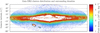 |
Fig. 1. Distribution of the 2 129 659 clusters of objects extracted from the Gaia DR2 catalogue. They are composed of three and four images that pass the soft astrometric test (see Sect. 2) that have a maximum angular separation between components that is smaller than 6″, that have absolute differences in G magnitudes of < 4 mag, and that are found in regions of the celestial sphere where the mean field density is lower than 6 × 10⁴ objects deg−2. Lower density regions near the galactic centre can be explained by the filtering occurring in the on-board processing in order to prevent memory from saturating in such very dense regions of the sky (Gaia Collaboration 2016). |
The production of the list of clusters is based on a search for neighbours around each of the Gaia DR2 sources that passed the soft astrometric test5. All combinations of three or four images were considered to produce the final list of clusters as the deflecting galaxy or contaminating stars might be present within the identified clusters.
Each cluster was then assigned a unique identifier based on the mean position of its constituent sources. The common convention of taking the position of the brightest image as an identifier for GL systems was not adopted here as it would lead to ambiguities in identifying clusters for which all combinations of images were explored. Figure 1 illustrates the distribution of the 2 129 659 clusters derived from Gaia DR2, amongst which 2 058 962 have three components and 70 697 have four components. Also depicted are the mean field densities that are associated with each of these clusters.
3. Identification of lens candidates from supervised learning method
After we defined the list of clusters, the second step in our methodology to perform a blind search for new GLs was the assignment of a discriminating value, called the extremely randomized trees (ERT) probability, to each cluster. These ERT probabilities, P, do not constitute probabilities in a mathematical sense and should rather be viewed as a figure of merit or as a score that reflects the ability of the clusters to be matched to the image positions and relative magnitudes produced from simulations of lens systems (see Sect. 3.1). They can, however, be translated into expected ratios of identification of GLs and to expected ratios of misclassification of groups of stars as GLs through the use of an appropriate cross-validation procedure.
3.1. Catalogue of simulated gravitational lenses
Supervised learning methods aim to automatically discover the relations that may exist between a set of input attributes and an associated outcome value based on a collection of training instances. The more complete and representative the learning set of observations, the fairer and more accurate the resulting predictions are (e.g. Beck et al. 2017). Training sets can be constructed either directly by using observational data or by using simulations. Regarding the specific problem of the identification of GL candidates, the limited number of 44 known quadruply-imaged systems from the list of Ducourant et al. (2018), of which only 19 have more than two images that are detected in Gaia DR2, forces us to rely on simulations to cover the input space of attributes in a satisfying manner.
To construct our training set, we consider a non-singular isothermal ellipsoid lens model in the presence of an external shear (hereafter NSIEg lens model, Kormann et al. 1994; Kovner 1987, see Appendix A for a concise description). This model has been proven to be well suited for reproducing the relative positions and flux ratios of the lensed images when the deflector is a massive late-type galaxy. A consequence of choosing this specific model is that the GL candidates we can identify through supervised learning methods will be restricted to systems that can be described well by this particular model. However, this does not constitute a major drawback to our implementation as most of the known lens systems are generally described well by this particular model.
Accordingly, we simulated 106 623 188 GL systems having four observable images based on a plausible range of parameters for the NSIEg lens model as listed in Table 2. For completeness, we note that a redundancy exists amongst the produced simulated GL systems. This is a natural consequence of a NSIEg lens model as, for example, all lens models with a shear orientation of π − ω and source position ( − xs, ys) are the horizontal reflections of models with a shear orientation of ω and a source position of (xs, ys).
Range of parameters explored to produce the simulated lens catalogues from a NSIEg lens model.
3.2. Extremely randomized tree supervised learning models
Extremely randomized tree probabilities are derived from a tree-based machine learning algorithm that relies on the assumption that the aggregation of the predictions of several weak, strongly randomized trees can compete or even surpass more sophisticated methods like artificial neural networks (Haykin 1998) or support vector machines (Cortes & Vapnik 1995). This assumption was initially supported by Mingers (1989) and was later successfully implemented in the bootstrap aggregating meta-algorithm (Breiman 1996) and in random forests (Breiman 2001). The usual classification and regression trees (CARTs) select at each node of the tree the attribute and cut-value within this attribute that best split the learning set of observations associated with this node according to a given score measure (e.g. the reduction of the variance in regression problems or the information gain in classification problems); instead, the ERT algorithm picks up a subset of K random attributes as well as a random cut-point within each of these attributes so as to select the split that maximizes the given score measure (Geurts et al. 2006). The algorithm ends when no more than nmin training observations remain in all leaf nodes. The aggregation of the predictions of N trees (a majority vote in our case) then lessens the variance of the ERT, in the sense that it prevents the model from being too specific to the learning set of observation we used while not being able to generalize the learned relations over unseen observations.
As we expect some of the lensed images to be missing from Gaia DR2 (see Table 1 for examples), all combinations of three and four images were considered for building the ERT. Also, as the central and strongly de-magnified image produced in NSIEg-like GLs is often out of reach of the Gaia photometric sensitivity, it was not taken into account. These ERT models are referred to in the following as ABCD, ABC, ABD, ACD, and BCD, where A, B, C, and D identify the images we used during the learning phase of the corresponding ERT sorted in ascending order of G magnitude.
All ERT models were trained using a learning set (LS) of observations composed of half the number of simulations we described in Sect. 3.1, plus an equal number of contaminant observations for which both the image positions and magnitudes were randomly drawn from a uniform distribution. We note that these simulated contaminants are still restricted to have an absolute difference in magnitude (ΔG) lower than 4 mag, in agreement with the requirements we developed in Sect. 2. The other half of the simulations is then kept as a test set (TS) of observations for cross-validation purpose, after being complemented by the addition of simulated contaminants. It is important to note here that neither LS nor TS follows a realistic distribution of positions and magnitudes as this would require, for example, the distribution of the eccentricity of the lensing galaxy or the properties of clusters of stars to be taken into account. These sets were solely designed with the aim of identifying the regions of the input space of parameters (i.e. relative positions and fluxes) where GLs and contaminants are located through the use of the ERT.
We then added a Gaussian noise to the image positions, σxy, and magnitudes, σG, for each of the LS and TS configurations before discarding some of their images in order to create the input instances used in the ABCD, ABC, ABD, ACD, and BCD models. These configurations are then normalized through an orthogonal transformation and a scaling to have their brightest image (image A) repositioned at (0, 0) along with a magnitude of 0 and their faintest image (image C or D, depending on the number of images of the configuration) repositioned at (1, 0).
The addition of noise to the simulations in the present case is not designed to take into account the astrometric and photometric uncertainties of Gaia DR2, which are actually much lower than the noise we introduced. Rather, this noise was added to deal with the possible imperfections of the NSIEg model, and to enable the machine learning method to deal with lenses that depart from this idealized model (e.g. due to substructures in the deflecting galaxies or to the inherent fact that the NSIEg lens model only constitutes an approximation of GLs whose deflectors are late-type galaxies). Similarly, the noise added to the magnitudes reflects the fact that micro-lensing events frequently occur due to galaxy substructures. Also, because of the difference in the optical paths of the lensed images, time delays exist between each of them, such that if the deflected source is a variable object, as quasars are, discrepancies would exist between our instantaneous noiseless simulations and real observations.
Regarding the ERT model ABCD, the set of input attributes is composed of the normalized images positions (xB,yB) and (xC,yC); of the normalized G magnitudes GB, GC, GD; and of their respective differences (xB−xC,yB−yC), GC − GB, GD − GB, and GD − GC. We recall that, because of the normalization procedure, xA = yA = yD = GA = 0, while xD = 1. The attributes used in the ERT model ABC is then similarly given by (xB, yB), GB, GC, and GC − GB, from which the attributes used in the ABD, ACD, and BCD models can be easily extrapolated.
The parameters of the ERT models (i.e. N, K, and nmin) as well as the level of noise we add to each of the LS and TS configurations, σxy and σG, were chosen in a heuristic way based on the identification performance of a validation set (VS) of observations, composed of the known lensed systems having four detections in Gaia DR26 (see Table 1) and of 106 clusters we randomly extracted from Gaia DR2 with a size smaller than 30″ and ΔG < 4 mag. Various combinations of these parameters were probed in the ranges N ∈ [10,1000], K ∈ [2,12], nmin ∈ [2,8], σG ∈ [0,1], and σxy ∈ [0,0.1 s], where s stands for the lens size. The set of parameters we selected regarding the ABCD models, N = 100, K = 12, nmin = 2, σxy = 0.01s and σG = 0.25, yield a satisfactory fraction of 75% of GLs that are correctly identified along with a misclassification rate of clusters of stars as GLs of 0.625% if P > 0.9. Not surprisingly, tests performed on the ABC, ABD, ACD, and BCD models lead to the same set of parameters, with the exception of K = 5, though the associated identification capabilities are now largely hampered.
3.3. Performance of the identification of known and simulated gravitational lenses
The performance of each model in classifying GL candidates were assessed by computing, for each of them, the fraction of GLs that are correctly identified (the true positive rate) and the fraction of clusters of stars that are misclassified as GLs (the false positive rate). By reporting the true and false positive rates (hereafter TPR and FPR, respectively) that are associated with all ERT probabilities in a graph, we obtain the receiver operating characteristics (ROC) curves, shown in Fig. 2. In the same figure, the area under the ROC curve (AUC) is a commonly used measure of the classification capability of each model. For completeness, we note that some simulated contaminants from our training set cannot be differentiated from the relative image positions and fluxes produced through NSIEg lens models. Regarding our ERT models, this has the effect of decreasing the TPR evaluated on the test set while increasing the associated FPR. Even so, as this degeneracy is seen in real observations, we decided not to remove these ambiguous simulations from our training set.
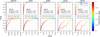 |
Fig. 2. Receiver operating characteristics (ROC) curve of the ABCD, ABC, ABD, ACD, and BCD models based on the test set (TS) and validation set (VS) of observations. The upper panels show the entire ROC curves, whereas the lower panels concentrate on the low FPR regions of each curve. The classification performances of each model is evaluated through the computation of the area under each of the TS–ROC and VS–ROC curves (AUC). |
We can see from Fig. 2 and Table 1 that the ERT model ABCD is able to identify 12 of the 13 known GLs (92.3%) and 92.5% of the simulated GLs along with a FPR that is below 1% if P > 0.84. The associated AUC (0.99503 if evaluated on the validation set or 0.99742 if evaluated on the test set) can be compared with the 0.98 obtained by the best lens classifier of the Strong Gravitational Lens Finding Challenge (Lanusse et al. 2018) where a FPR of 1% is associated with a TPR of 90% (Metcalf et al. 2018). However, these numbers should be taken with care given the difficulties in equitably comparing two models designed for different instruments, having different angular resolutions and photometric sensitivities, and working directly on images on the one hand and on reduced data on the other. In a more recent work, Wynne & Schechter (2018) achieve a TPR of 80% along with a FPR of 2% by directly modelling the quadruple lens systems through the fit of a right hyperbola to the observed relative positions of the lensed images (Witt 1996). Cuts on the resulting axis ratio, q, and on the scatter of the observed images around the fitted hyperbola being then used to select GL candidates. These comparisons demonstrate the efficiency of the approach adopted in the present work and more particularly of the ERT on this particular problem. These results also demonstrate the huge potential of Gaia regarding the identification of GLs, mostly coming from its impressive astrometric and photometric precision.
The ERT models ABC and ABD provide FPRs of 5.83% and of 7.48%, respectively, on the validation set if they are associated with a TPR of 75%. The FPR associated with the test set are 5.08% and of 7.74%, respectively, for the same TPR. Nevertheless, if a TPR of 75% is considered for the models ACD and BCD, then the corresponding FPR computed on the validation set rises to ∼20% (∼10% on the test set). These larger FPRs apparently come from the intrinsic difficulty that the ERT have in identifying GLs for which the two brightest images are not seen together, as illustrated by the ROC curves computed on the test set. Also, the discrepancies noticed in the ROC curves computed based on the test set, on the one hand, and on the validation set, on the other hand, can be explained by the statistical fluctuations due to the low number of known GLs present in the validation set (13) and by the fact that they contain different populations of lenses (i.e. the validation set contains a realistic population of lenses, whereas the test set contains a population of simulated lenses coming from a uniform coverage of the NSIEg parameters). We note that FPRs as low as a few per cent still lead to a large number of contaminant observations in the final catalogue, owing to the 2 × 10⁶ clusters identified in Gaia DR2. The appropriate filtering of these numerous contaminants is described in Sect. 3.4.
In addition to the overall performance of our approach, some of the known lenses from Table 1 are still being assigned low ERT probabilities, P, namely J0630-1201 (PABC = 0.58), RXJ0911+0551 (PACD = 0.67), RXJ1131–1231 (PABCD = 0.65), and WISE025942.9–163543 (PABD = 0.45). The first of these, J0630–1201, is a recently discovered GL composed of five lensed images and two deflecting galaxies (Ostrovski et al. 2018), which can thus not be reproduced through a single NSIEg lens model. The GLs RXJ0911+0551 and RXJ1131–1231 have flux ratios that are difficult to reproduce without including microlensing by small-scale structures in the lens galaxy (Keeton et al. 2003). The fact that RXJ1131-1231 obtains an ERT probability of PABD = 0.93 once image C is discarded also supports this hypothesis. The study of the recently discovered GL WISE025942.9–163543 currently remains very limited, though the preliminary modelling performed by Schechter et al. (2018) using a non-singular isothermal sphere lens model in the presence of external shear (i.e. NSIEg lens model with q = 1 and s = 0) has already highlighted the difficulties in reproducing the observed flux ratios, even if the image positions can be fairly well reproduced by this kind of model (Wynne & Schechter 2018). The modelling that we have performed using a NSIEg lens model has led to the same conclusion.
We also note that two GL candidates, PS1J205143–111444 and WGD2141–4629, were already present in the original list of Ducourant et al. (2018). These candidates obtain maximum ERT probabilities of PABD = 0.01 and of PABC = 0.62, respectively. Whereas PS1J205143–111444 is probably not a GL that is reproducible through a NSIEg lens model, the lensing nature of WGD2141–4629 remains uncertain though highly improbable because of the non-negligible, opposite proper motions of two of its images, while one of them is astrometrically well behaved (i.e. astrometric excess noise of ϵ = 0 mas). More recently, Agnello & Spiniello (2018) discovered two new quadruply-imaged lens candidates, WG210014.9–445206.4 and WG021416.37–210535.3, that are not part of our input list of candidate lenses taken from Ducourant et al. (2018). These candidates obtain maximum ERT probabilities of PABC = 0.4 and PABC = 0.94, respectively. Even though the lensing nature of WG210014.9–445206.4 looks very promising, it was not recognized by our method. Possible reasons are the finite identification rate (TPR) of the ERT or the hardly reproducible relative positions and magnitudes of this system through a NSIEg lens model.
Finally, we mention that the ERT models described here differ significantly from those we built and used in Paper I (Krone-Martins et al. 2018) as we adjusted our model to known GLs contained in Gaia DR2, whereas only SDSS J1004+4112 had all its components detected in Gaia DR1.
3.4. Identification of new gravitational lens candidates
Finally, we applied the methodology developed in this work to the 2 129 659 clusters we extracted from the Gaia DR2 with a view of identifying GL candidates. The resulting catalogue of clusters, along with their associated ERT probabilities, is further described in Appendix B; the distributions of these ERT probabilities regarding the clusters and the known lenses they contain are also provided in Fig. 3. From this figure, we can see that most of the clusters have low ERT probabilities; for example, 43.34% of the clusters composed of three images and 89.52% of the clusters composed of four images have ERT probabilities P < 0.2. Conversely, 10 of the 11 known lenses composed of four Gaia detections and 36 of the 50 known lenses composed of three detections7 have an ERT probability P > 0.8. We note that the large number of clusters having high ERT probabilities amongst the clusters composed of three images is due to the choice we made to consider a single ERT probability that is taken as the maximum of the probabilities that are returned by the ABC, ABD, ACD, and BCD models. This choice is justified by the fact that if we observed a genuine quadruply-imaged quasar having only three detections in Gaia DR2, we do not know which of the images was unobserved and consequently, in a conservative approach, we have to consider the ERT model that worked best.
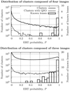 |
Fig. 3. Distribution of the 70 697 clusters composed of four images and 2 058 962 clusters composed of three images extracted from the Gaia DR2 (see Sect. 2) with respect to their ERT probabilities (solid line). The distribution of the known lenses are represented as boxes, whereas the distribution of the 6,944 clusters resulting from the cross-match we performed between our entire list of clusters and our compiled list of quasars is depicted as a dotted line in each graph (see Sect. 3.4.2). In cases where clusters are composed of three images, the ERT probability corresponds to the maximum of the ERT probabilities returned by the ABC, ABD, ACD, and BCD models. |
List of GL candidates.
In the following, we do not aim to provide an exhaustive list of the GLs that are contained in this catalogue, but rather to provide the community with a very pure list of GL candidates at the expense of a lower completeness. We note again here that GLs having prominent substructures in the lensing galaxy, multiple lensing galaxies, and/or high variability will be hardly identified by the ERT as these are often not modelled well with NSIEg lens models.
3.4.1. Systematic blind search of gravitational lenses composed of four images
In this first approach, our aim was to systematically and blindly identify GL candidates that are composed of four Gaia detections while sharing common properties with the set of known lenses from Table 1. The reason for considering these four image candidates apart from those composed of three images lies first in the benefit we can draw from the excellent performance of the ABCD ERT model. Furthermore, it is impossible to have a systematic search for lenses in the triplet regime because of the relatively high FPR of the ABC, ABD, ACD, and BCD ERT models (5% ≲ FPR ≲ 20%) and because of the numerous clusters to which they will be applied (2 058 962 clusters composed of three images).
According to the mean density of objects found around known GLs (see Table 1) and based on the maximum absolute difference in colour between their lensed images, Δ(GBP − GRP), we first restricted our four-image candidates to regions where ρ < 3 × 10⁴ objects deg−2, while having a maximum absolute difference in colour Δ(GBP − GRP)< 0.4 mag, when available. Similarly, we also required our candidates to have an ERT probability of P > 0.9. Of the ten clusters satisfying these criteria, seven are known lenses (2MASS J11344050–2103230, WGD2038–4008, HE0435-1223, PG1115+080, B1422+231, 2MASS J13102005–1714579, and J1721+8842), while three clusters (numbered [4], [15] and [18] in the finding charts from Fig. 4 and Table 3) are new GL candidates. This first analysis already proved the identification capability of our approach based solely on data products from the Gaia DR2. Nevertheless, candidate number [4] is probably not a GL in our opinion, mostly because of the red colour of its constituent images. Similarly, the DSS2 images of candidates [15] and [18] do not have sufficient angular resolution to determine their lensing nature. Even so, their relative image positions and fluxes are compatible with those produced by NSIEg-like lenses.
3.4.2. Search for gravitational lenses around quasars and quasar candidates
A systematic blind search for new lensed systems where only three images are detected in Gaia is not feasible given the numbers we provided in Fig. 3. Instead, constraints from external catalogues have to be used so as to lessen the number of candidate clusters. We know that lensed sources from GLs are always extragalactic objects, either active galactic nuclei (AGN) or galaxies. The latter, however, are extended objects of low surface brightness that will accordingly not be detected by Gaia. We thus performed a cross-match between our entire list of clusters, the compiled quasars list from Krone-Martins et al. (2018), and the C75 and R90 WISE AGN catalogue from Assef et al. (2018). The first of these lists consists of 3 112 975 candidate quasars compiled from the Million Quasars catalogue (Flesch 2015, 2017), from a photometric selection of WISE AGN (Secrest et al. 2015), from the third release of the Large Quasar Astrometric Catalogue (Souchay et al. 2015) and from the twelfth data release of the SDSS quasar catalogue (Pâris et al. 2017). The R90 and C75 catalogues consist of 4 543 530 and 20 907 127 WISE AGN candidates, respectively, selected across the whole extragalactic sky based solely on mid-infrared colours. The R90 catalogue has a reliability of 90%, while the C75 catalogue has a completeness of 75%.
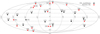 |
Fig. 5. Distribution of the known and new candidate GLs in Galactic coordinates. The numbers in square brackets refer to the candidate numbers from Table 3 and Fig. 4. |
This cross-match resulted in 6944 clusters composed of three or four images for which at least one of them has a counterpart in our compiled list of quasars. Figure 3 gives the distributions of the ERT probabilities of these clusters. We note that these distributions are simply scaled versions of the distributions we obtained if no cross-match was performed, meaning that the vast majority of the clusters remain contaminants and not gravitational lens systems. Based on the same figure, we decided to set a threshold on the ERT probability of P ≥ 0.6, which ensures that most of the known lenses will be detected, with the exception of four over a total of 61 known systems: 11 with four Gaia detections, 44 combinations of three images from these 11 systems, and 6 with three Gaia detections). A visual inspection of the 2572 resulting clusters composed of more than two images then yielded the GL candidates numbered [8], [11], [12], [16], [17], [19], [20], [23], [25], [26], [28], and [30] from Fig. 4 and Table 3. Despite the low cut we set on the ERT probability (P ≥ 0.6), we note that out of the 12 candidates we propose, 10 have ERT probabilities higher than or equal to 0.88, assessing the interest of the ERT for identifying GL events, even in the case where only three images are detected.
Finally, we note that candidate number [12] was already present in Krone-Martins et al. (2018) and has since been spectroscopically confirmed as a GL (Wertz et al. 2018). Five other candidates were also spectroscopically confirmed through Keck/LRIS observations after the submission of this paper (candidates numbered [11], [17], [23], [25], and [26], Krone-Martins et al., in prep.). Three of these new GLs (numbered [11], [23], and [26]) were also independently confirmed by Lemon et al. (2019). Candidate number [26], however, is a doubly-imaged quasar that should thus be considered a false positive from the ERT. On the other hand, the lensing nature of two candidates were denied (candidates numbered [16] and [30]) and led to inconclusive results regarding two others (candidates numbered [19] and [28]). The lensing nature of other candidates currently remains uncertain but plausible.
4. Conclusions
In this work, we aimed to discover quadruply-imaged lens candidates through the use of a supervised learning method, called extremely randomized trees (ERT), applied over the whole Gaia DR2. To train the ERT models, we simulated the relative positions and flux ratios of 106,623,188 quadruply-imaged systems based on a non-singular isothermal ellipsoid lens model in the presence of external shear. The performance of our ERT models were probed using simulations and real observations from Gaia DR2. From the known quadruply-imaged systems having all components detected in Gaia DR2, 12 out of 13 are successfully recovered by our method along with a misclassification rate of fortuitous clusters of stars as lenses that is below 1%. Similarly, 92.5% of the simulated lens systems are identified with the same misclassification rate.
The performance of our ERT models in identifying quadruply-imaged systems where only three components are detected in Gaia DR2 is evaluated by removing one image from each of the simulated and known quadruply-imaged systems. This resulted in the correct identification of 10 out of 13 known lensed systems with a misclassification rate below 7.5% when the two brightest images of the lens were observed together and ∼20% otherwise. For the same identification rate, tests performed on simulations provided a similar misclassification rate of 7.74% for configurations where the two brightest images are present and ∼10% otherwise.
We applied our ERT models to 70 697 clusters composed of four images and to 2 058 962 clusters composed of three images we extracted from the Gaia DR2. Beforehand, a filtering of the Gaia DR2 sources was used in order to remove non-stationary objects based on the parallax and proper motions of each source. Clusters were also restricted to have a maximum separation between images of 6″, a maximum absolute difference of G magnitude between components below 4 mag, and locations in regions of the sky where the mean field density is below 6 × 10⁴ objects deg−2.
Benefiting from the high identification rate of our ERT model in cases where all four components from quadruply-imaged systems are detected, and from the low associated misclassification rate of clusters of stars as gravitational lens we succeeded in isolating seven known gravitational lenses composed of four images based on simple cuts in the mean field density, in the maximum absolute difference in colour, and in the discriminant value provided by the ERT model. Three clusters are also retrieved through this straight selection and are hence promoted as plausible lens candidates.
In addition to this Gaia-only approach, we performed a cross-match between our list of clusters from Gaia DR2 sources, and compiled lists of spectroscopically confirmed quasars and photometric quasar candidates. We visually inspected the resulting 2572 clusters for which the ERT models predicted a reasonably good agreement between these clusters and the relative positions and flux ratios from a non-singular isothermal ellipsoid lens model in the presence of an external shear.
The method presented here succeeded in finding 15 highly probable quadruply-imaged quasar candidates, five of which have recently been spectroscopically confirmed. The low number of lens candidates we identified from Gaia data, with respect to the Finet & Surdej (2016) predictions, can mostly be explained by the fact that the majority of gravitational lenses present in Gaia DR2 have less than three lensed images published in the catalogue, as shown by Ducourant et al. (2018). We expect that Gaia DR3 and later DR4 will improve on this, due to a less stringent filtering of the published sources and improved processing. Meanwhile, this method can be used on other catalogues, as it solely relies on astrometric and photometric data. Applications are already foreseen for the upcoming Gaia DR3 and combinations of already available catalogues (e.g. PanSTARRS, DES, SDSS, and Gaia DR2).
For this purpose we used a subdivision of the celestial sphere based on the Hierarchical Triangular Mesh (Kunszt et al. 2001).
J2145+6345 was not used to build our ERT models or to determine the level of noise to add to our simulations as this lens had not been published at the time of submission.
Forty-four of the known gravitational lens systems composed of three images come from the combination of the images of the 11 known systems composed of four images while 6 are known systems for which an image was undetected (see Table 1 for details).
Acknowledgments
LD and JS acknowledge support from the ESA PRODEX Programme “Gaia-DPAC QSOs” and from the Belgian Federal Science Policy Office. AKM acknowledges the support from the Portuguese Fundação para a Ciência e a Tecnologia (FCT) through grants SFRH/BPD/74697/2010 and PTDC/FIS-AST/31546/2017, from the Portuguese Strategic Programme UID/FIS/00099/2013 for CENTRA, from the ESA contract AO/1-7836/14/NL/HB, and from the Caltech Division of Physics, Mathematics and Astronomy for hosting a research leave during 2017–2018, when this paper was prepared. OW is supported by the Humboldt Research Fellowship for Postdoctoral Researchers. SGD and MJG acknowledge partial support from the NSF grants AST-1413600 and AST-1518308, and the NASA grant 16-ADAP16-0232. The work of DS was carried out at the Jet Propulsion Laboratory, California Institute of Technology, under a contract with NASA. We acknowledge partial support from “Actions sur projet INSU-PNGRAM”, and from the Brazil-France exchange programmes Fundação de Amparo à Pesquisa do Estado de São Paulo (FAPESP) and Coordenação de Aperfeiçoamento de Pessoal de Nível Superior (CAPES) – Comité Français d’Évaluation de la Coopération Universitaire et Scientifique avec le Brésil (COFECUB). This work has made use of the computing facilities of the Laboratory of Astroinformatics (IAG/USP, NAT/Unicsul), whose purchase was made possible by the Brazilian agency FAPESP (grant 2009/54006-4) and the INCT-A, and we thank the entire LAi team, especially Carlos Paladini, Ulisses Manzo Castello, Luis Ricardo Manrique, and Alex Carciofi for their support. This work has made use of results from the ESA space mission Gaia, the data from which were processed by the Gaia Data Processing and Analysis Consortium (DPAC). Funding for the DPAC has been provided by national institutions, in particular the institutions participating in the Gaia Multilateral Agreement. The Gaia mission website is http://www.cosmos.esa.int/gaia. Some of the authors are members of the Gaia Data Processing and Analysis Consortium (DPAC).
References
- Agnello, A., & Spiniello, C. 2018, MNRAS, submitted [arXiv:1805.11103] [Google Scholar]
- Agnello, A., Lin, H., Kuropatkin, N., et al. 2018a, MNRAS, 479, 4345 [NASA ADS] [CrossRef] [Google Scholar]
- Agnello, A., Schechter, P. L., Morgan, N. D., et al. 2018b, MNRAS, 475, 2086 [NASA ADS] [CrossRef] [Google Scholar]
- Alam, S., Albareti, F. D., Allende Prieto, C., et al. 2015, ApJS, 219, 12 [NASA ADS] [CrossRef] [Google Scholar]
- Alard, C. 2006, ArXiv e-prints [arXiv:astro-ph/0606757] [Google Scholar]
- Anguita, T., Schechter, P. L., Kuropatkin, N., et al. 2018, MNRAS, 480, 5017 [NASA ADS] [Google Scholar]
- Assef, R. J., Stern, D., Noirot, G., et al. 2018, ApJS, 234, 23 [NASA ADS] [CrossRef] [Google Scholar]
- Avestruz, C., Li, N., Lightman, M., Collett, T. E., & Luo, W. 2017, ArXiv e-prints [arXiv:1704.02322] [Google Scholar]
- Bailer-Jones, C. A. L., Andrae, R., Arcay, B., et al. 2013, A&A, 559, A74 [NASA ADS] [CrossRef] [EDP Sciences] [Google Scholar]
- Bañados, E., Venemans, B. P., Mazzucchelli, C., et al. 2018, Nature, 553, 473 [NASA ADS] [CrossRef] [Google Scholar]
- Beck, R., Lin, C. A., Ishida, E. E. O., et al. 2017, MNRAS, 468, 4323 [NASA ADS] [CrossRef] [Google Scholar]
- Bellm, E., & Kulkarni, S. 2017, Nat. Astron., 1, 0071 [CrossRef] [Google Scholar]
- Bertin, E., Delorme, P., & Bouy, H. 2012, Astrophys. Space Sci. Proc., 29, 71 [NASA ADS] [CrossRef] [Google Scholar]
- Bolton, A. S., Burles, S., Koopmans, L. V. E., et al. 2008, ApJ, 682, 964 [NASA ADS] [CrossRef] [Google Scholar]
- Bonnarel, F., Fernique, P., Bienaymé, O., et al. 2000, A&AS, 143, 33 [NASA ADS] [CrossRef] [EDP Sciences] [Google Scholar]
- Breiman, L. 1996, Mach. Learn., 24, 123 [Google Scholar]
- Breiman, L. 2001, Mach. Learn., 45, 5 [CrossRef] [Google Scholar]
- Chambers, K. C., Magnier, E. A., Metcalfe, N., et al. 2016, ArXiv e-prints [arXiv:1612.05560] [Google Scholar]
- Cortes, C., & Vapnik, V. 1995, Mach. Learn., 20, 273 [Google Scholar]
- Dalal, N., & Kochanek, C. S. 2002, ApJ, 572, 25 [NASA ADS] [CrossRef] [Google Scholar]
- Dark Energy Survey Collaboration, Abbott, T., Abdalla, F. B., et al. 2016, MNRAS, 460, 1270 [NASA ADS] [CrossRef] [Google Scholar]
- de Souza, R. E., Krone-Martins, A., dos Anjos, S., Ducourant, C., & Teixeira, R. 2014, A&A, 568, A124 [NASA ADS] [CrossRef] [EDP Sciences] [Google Scholar]
- Drake, A. J., Djorgovski, S. G., Mahabal, A., et al. 2009, ApJ, 696, 870 [NASA ADS] [CrossRef] [MathSciNet] [Google Scholar]
- Ducourant, C., Wertz, O., Krone-Martins, A., et al. 2018, A&A, 618, A56 [NASA ADS] [CrossRef] [EDP Sciences] [Google Scholar]
- Einstein, A. 1936, Science, 84, 506 [NASA ADS] [CrossRef] [PubMed] [Google Scholar]
- Finet, F., & Surdej, J. 2016, A&A, 590, A42 [NASA ADS] [CrossRef] [EDP Sciences] [Google Scholar]
- Flesch, E. W. 2015, PASA, 32, e010 [NASA ADS] [CrossRef] [Google Scholar]
- Flesch, E. W. 2017, VizieR Online Data Catalog: VII/280 [Google Scholar]
- Gaia Collaboration (Prusti, T., et al.) 2016, A&A, 595, A1 [NASA ADS] [CrossRef] [EDP Sciences] [Google Scholar]
- Gaia Collaboration (Brown, A. G. A., et al.) 2018, A&A, 616, A1 [NASA ADS] [CrossRef] [EDP Sciences] [Google Scholar]
- Geurts, P., Ernst, D., & Wehenkel, L. 2006, Mach. Learn., 63, 3 [Google Scholar]
- Gilman, D., Birrer, S., Treu, T., & Keeton, C. R. 2018, MNRAS, 481, 819 [NASA ADS] [CrossRef] [Google Scholar]
- Hartley, P., Flamary, R., Jackson, N., Tagore, A. S., & Metcalf, R. B. 2017, MNRAS, 471, 3378 [NASA ADS] [CrossRef] [Google Scholar]
- Haykin, S. 1998, Neural Networks: A Comprehensive Foundation, 2nd edn. (Upper Saddle River, NJ, USA: Prentice Hall PTR) [Google Scholar]
- Inada, N., Oguri, M., Shin, M.-S., et al. 2012, AJ, 143, 119 [NASA ADS] [CrossRef] [Google Scholar]
- Jacobs, C., Glazebrook, K., Collett, T., More, A., & McCarthy, C. 2017, MNRAS, 471, 167 [NASA ADS] [CrossRef] [Google Scholar]
- Jauzac, M., Harvey, D., & Massey, R. 2018, MNRAS, 477, 4046 [NASA ADS] [CrossRef] [Google Scholar]
- Jones, D. O., Scolnic, D. M., Riess, A. G., et al. 2018, ApJ, 857, 51 [NASA ADS] [CrossRef] [Google Scholar]
- Keeton, C. R., & Kochanek, C. S. 1998, ApJ, 495, 157 [NASA ADS] [CrossRef] [Google Scholar]
- Keeton, C. R., Gaudi, B. S., & Petters, A. O. 2003, ApJ, 598, 138 [NASA ADS] [CrossRef] [Google Scholar]
- Kirkpatrick, J. D., Reid, I. N., Liebert, J., et al. 1999, ApJ, 519, 802 [NASA ADS] [CrossRef] [Google Scholar]
- Kirkpatrick, J. D., Schneider, A., Fajardo-Acosta, S., et al. 2014, ApJ, 783, 122 [NASA ADS] [CrossRef] [Google Scholar]
- Kormann, R., Schneider, P., & Bartelmann, M. 1994, A&A, 284, 285 [NASA ADS] [Google Scholar]
- Kovner, I. 1987, ApJ, 312, 22 [NASA ADS] [CrossRef] [Google Scholar]
- Krone-Martins, A., Ducourant, C., Teixeira, R., et al. 2013, A&A, 556, A102 [NASA ADS] [CrossRef] [EDP Sciences] [Google Scholar]
- Krone-Martins, A., Delchambre, L., Wertz, O., et al. 2018, A&A, 616, L11 [NASA ADS] [CrossRef] [EDP Sciences] [Google Scholar]
- Kunszt, P. Z., Szalay, A. S., & Thakar, A. R. 2001, in Mining the Sky, eds. A. J. Banday, S. Zaroubi, & M. Bartelmann, 631 [CrossRef] [Google Scholar]
- Lanusse, F., Ma, Q., Li, N., et al. 2018, MNRAS, 473, 3895 [NASA ADS] [CrossRef] [Google Scholar]
- Lasker, B. M., Doggett, J., McLean, B., et al. 1996, in Astronomical Data Analysis Software and Systems V, eds. G. H. Jacoby, & J. Barnes, ASP Conf. Ser., 101, 88 [NASA ADS] [Google Scholar]
- Lee, C.-H. 2017, PASA, 34, e014 [NASA ADS] [CrossRef] [Google Scholar]
- Lemon, C. A., Auger, M. W., & McMahon, R. G. 2019, MNRAS, 483, 4242 [NASA ADS] [CrossRef] [Google Scholar]
- Meneghetti, M., Natarajan, P., Coe, D., et al. 2017, MNRAS, 472, 3177 [Google Scholar]
- Metcalf, R. B., Meneghetti, M., Avestruz, C., et al. 2018, ArXiv e-prints [arXiv:1802.03609] [Google Scholar]
- Mingers, J. 1989, Mach. Learn., 3, 319 [Google Scholar]
- More, A., Cabanac, R., More, S., et al. 2012, ApJ, 749, 38 [Google Scholar]
- More, A., Oguri, M., Kayo, I., et al. 2016, MNRAS, 456, 1595 [NASA ADS] [CrossRef] [Google Scholar]
- Ostrovski, F., Lemon, C. A., Auger, M. W., et al. 2018, MNRAS, 473, L116 [NASA ADS] [CrossRef] [Google Scholar]
- Paraficz, D., Courbin, F., Tramacere, A., et al. 2016, A&A, 592, A75 [NASA ADS] [CrossRef] [EDP Sciences] [Google Scholar]
- Pâris, I., Petitjean, P., Ross, N. P., et al. 2017, A&A, 597, A79 [NASA ADS] [CrossRef] [EDP Sciences] [Google Scholar]
- Peng, C. Y., Impey, C. D., Rix, H.-W., et al. 2006, ApJ, 649, 616 [Google Scholar]
- Pourrahmani, M., Nayyeri, H., & Cooray, A. 2018, ApJ, 856, 68 [NASA ADS] [CrossRef] [Google Scholar]
- Refsdal, S. 1964, MNRAS, 128, 307 [NASA ADS] [CrossRef] [Google Scholar]
- Schechter, P. L., Anguita, T., Morgan, N. D., Read, M., & Shanks, T. 2018, Res. Notes AAS, 2, 21 [NASA ADS] [CrossRef] [Google Scholar]
- Secrest, N. J., Dudik, R. P., Dorland, B. N., et al. 2015, ApJS, 221, 12 [NASA ADS] [CrossRef] [Google Scholar]
- Shajib, A. J., Birrer, S., Treu, T., et al. 2019, MNRAS, 483, 5649 [NASA ADS] [CrossRef] [Google Scholar]
- Skrutskie, M. F., Cutri, R. M., Stiening, R., et al. 2006, AJ, 131, 1163 [NASA ADS] [CrossRef] [Google Scholar]
- Sonnenfeld, A., Chan, J. H. H., Shu, Y., et al. 2018, PASJ, 70, S29 [NASA ADS] [CrossRef] [Google Scholar]
- Souchay, J., Andrei, A. H., Barache, C., et al. 2015, A&A, 583, A75 [NASA ADS] [CrossRef] [EDP Sciences] [Google Scholar]
- Suyu, S. H., Auger, M. W., Hilbert, S., et al. 2013, ApJ, 766, 70 [NASA ADS] [CrossRef] [Google Scholar]
- Tagore, A. S., Barnes, D. J., Jackson, N., et al. 2018, MNRAS, 474, 3403 [NASA ADS] [CrossRef] [Google Scholar]
- Tsalmantza, P., Karampelas, A., Kontizas, M., et al. 2012, A&A, 537, A42 [NASA ADS] [CrossRef] [EDP Sciences] [Google Scholar]
- Walsh, D., Carswell, R. F., & Weymann, R. J. 1979, Nature, 279, 381 [NASA ADS] [CrossRef] [PubMed] [Google Scholar]
- Wertz, O., Stern, D., Krone-Martins, A., et al. 2018, A&A, submitted [arXiv:1810.02624] [Google Scholar]
- Witt, H. J. 1996, ApJ, 472, L1 [NASA ADS] [CrossRef] [Google Scholar]
- Wright, E. L., Eisenhardt, P. R. M., Mainzer, A. K., et al. 2010, AJ, 140, 1868 [NASA ADS] [CrossRef] [Google Scholar]
- Wynne, R. A., & Schechter, P. L. 2018, MIT Undergrad. Res. J., submitted [arXiv:1808.06151] [Google Scholar]
- Zavala, J. A., Montaña, A., Hughes, D. H., et al. 2018, Nat. Astron., 2, 56 [NASA ADS] [CrossRef] [Google Scholar]
Appendix A: Non-singular isothermal ellipsoid lens model in the presence of an external shear
The non-singular isothermal ellipsoid lens model in the presence of an external shear (NSIEg) is characterized by κ, the dimensionless surface mass density projected in the lens plane and defined by
 (A.1)
(A.1)
where the coordinates (x, y) locate a position in the lens plane, s corresponds to the deflector core radius, q is the ratio of the minor to the major axes of the elliptical isodensity contours, and b is considered here as a normalizing factor. From Keeton & Kochanek (1998), the two components of the corresponding scaled deflection angle, α, are given by
 (A.2)
(A.2)
and
 (A.3)
(A.3)
where  is defined as the eccentricity of the isodensity contours, and ψ2 = q2(s2+x2) + y2. The contribution of more distant massive objects to the deflection is taken into account through an external shear term of the form
 (A.4)
(A.4)
where γ is the shear intensity and ω its orientation. Finally, the position θs = (xs,ys) of a point-like source is related to a lensed image position θ = (x,y) through the so-called lens equation
 (A.5)
(A.5)
and the associated magnification factor μ(θ) is then defined by
 (A.6)
(A.6)
where the Jacobian matrix A(θ) = ∂θs(θ)/∂θ is called the amplification matrix.
Appendix B: Gaia GraL catalogue of clusters from Gaia DR2 sources
The Gaia GraL catalogue of clusters from Gaia DR2 sources is available at the CDS. The catalogue is composed of all 2 129 659 clusters identified in Sect. 2 along with the ERT probabilities computed for each of them (see Sect. 3). For ease of identifying the images constituting each cluster and to facilitate the cross-match against other catalogues based on the individual components of the clusters, each entry from the catalogue corresponds to a single Gaia DR2 source within the cluster. Consequently, clusters composed of three and four images have, respectively, three and four associated entries in the catalogue along with the fields that are common to the cluster they belong to. The fields constituting each row of the catalogue are detailed in Table B.1.
Description of the fields contained in the Gaia GraL catalogue of clusters from Gaia DR2 sources.
Our objective here is not to provide a list of GL candidates, as we do in Sects. 3.4.1 and 3.4.2, but to provide the user with a catalogue that can easily provide hints on the lensing nature of some of the observational targets, at least regarding GLs that are reproducible through a NSIEg lens model. This approach also justifies the inclusion of clusters located in regions of the sky we know to be densely populated and where the contamination rate of GL candidates will typically be very high. The removal of the clusters having a field density higher than ρ > 3 × 10⁴ objects deg−2 effectively reduces their number by a factor of ten (205 004 remaining clusters).
To our knowledge, the present catalogue is the first to provide a discriminating value associated with each cluster that reflects the ability for a given GL model to reproduce the observed configuration of images. These ERT probabilities can provide a straight binary classification as, for example, 96.31% of the four-image configurations have P < 0.5, whereas 86.11% of the three-image configurations have P < 0.9. The threshold we set on P are obviously application-dependent and should be set in agreement with the ROC curves we described in Sect. 3. Finally, in a conservative approach, we do not set any cut on the difference in colour between images of the clusters, Δ(GBP − GRP). However, whenever they are available they provide an important criterion for identifying GLs as we do not expect the colours to vary much between the images of GLs (see Sect. 3.4 for examples).
All Tables
List of all spectroscopically confirmed quadruply-imaged systems having Nimg = 3, 4 components detected in Gaia DR2.
Range of parameters explored to produce the simulated lens catalogues from a NSIEg lens model.
Description of the fields contained in the Gaia GraL catalogue of clusters from Gaia DR2 sources.
All Figures
|
Fig. 1. Distribution of the 2 129 659 clusters of objects extracted from the Gaia DR2 catalogue. They are composed of three and four images that pass the soft astrometric test (see Sect. 2) that have a maximum angular separation between components that is smaller than 6″, that have absolute differences in G magnitudes of < 4 mag, and that are found in regions of the celestial sphere where the mean field density is lower than 6 × 10⁴ objects deg−2. Lower density regions near the galactic centre can be explained by the filtering occurring in the on-board processing in order to prevent memory from saturating in such very dense regions of the sky (Gaia Collaboration 2016). |
| In the text | |
|
Fig. 2. Receiver operating characteristics (ROC) curve of the ABCD, ABC, ABD, ACD, and BCD models based on the test set (TS) and validation set (VS) of observations. The upper panels show the entire ROC curves, whereas the lower panels concentrate on the low FPR regions of each curve. The classification performances of each model is evaluated through the computation of the area under each of the TS–ROC and VS–ROC curves (AUC). |
| In the text | |
|
Fig. 3. Distribution of the 70 697 clusters composed of four images and 2 058 962 clusters composed of three images extracted from the Gaia DR2 (see Sect. 2) with respect to their ERT probabilities (solid line). The distribution of the known lenses are represented as boxes, whereas the distribution of the 6,944 clusters resulting from the cross-match we performed between our entire list of clusters and our compiled list of quasars is depicted as a dotted line in each graph (see Sect. 3.4.2). In cases where clusters are composed of three images, the ERT probability corresponds to the maximum of the ERT probabilities returned by the ABC, ABD, ACD, and BCD models. |
| In the text | |
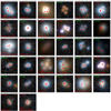 |
Fig. 4. Finding charts of the 17 known GLs and 15 GL candidates contained in our catalogue of clusters (Appendix B). They are ordered according to their ERT probabilities (upper left corner of each subplot). The common name of the known lenses is labelled in red in the lower left corner of each subplot, while the candidates we propose have their probabilities written in green fonts. Images [1], [2], [4–7], [9], [11], [13], [14], [16], [17], [19–23], [25–32] come from the Pan-STARRS survey (Chambers et al. 2016); images [12], [15], [18] come from the Digitized Sky Survey II (Lasker et al. 1996); and images [3], [8], [10], [24] come from the DES (Dark Energy Survey Collaboration et al. 2016). All images were collected from the ALADIN sky atlas (Bonnarel et al. 2000) in a field of view of 10.8″ × 10.8″ centred around the mean coordinates of the GL where east is to the left and north is up. Points are scaled according to the relative flux of the components with respect to the brightest image of each configuration. |
| In the text | |
|
Fig. 5. Distribution of the known and new candidate GLs in Galactic coordinates. The numbers in square brackets refer to the candidate numbers from Table 3 and Fig. 4. |
| In the text | |
Current usage metrics show cumulative count of Article Views (full-text article views including HTML views, PDF and ePub downloads, according to the available data) and Abstracts Views on Vision4Press platform.
Data correspond to usage on the plateform after 2015. The current usage metrics is available 48-96 hours after online publication and is updated daily on week days.
Initial download of the metrics may take a while.