| Issue |
A&A
Volume 622, February 2019
|
|
|---|---|---|
| Article Number | A126 | |
| Number of page(s) | 14 | |
| Section | Stellar structure and evolution | |
| DOI | https://doi.org/10.1051/0004-6361/201833728 | |
| Published online | 07 February 2019 | |
Optical spectroscopic and polarization properties of 2011 outburst of the recurrent nova T Pyxidis⋆
1
Indian Institute of Astrophysics, 560 034 Bangalore, India
e-mail: This email address is being protected from spambots. You need JavaScript enabled to view it.
2
Pondicherry University, R.V. Nagar, Kalapet 605014, Puducherry, India
3
Inter-University Center for Astronomy and Astrophysics, Post Bag 4, Ganeshkhind, 411 007 Pune, India
Received:
28
June
2018
Accepted:
17
December
2018
Abstract
Aims. We aim to study the spectroscopic and ionized structural evolution of T Pyx during its 2011 outburst, and also study the variation in degree of polarization during its early phase.
Methods. Optical spectroscopic data of this system obtained from day 1.28–2415.62 since discovery, and optical, broadband imaging polarimetric observations obtained from day 1.36–29.33 during the early phases of the outburst were used in the study. The physical conditions and the geometry of the ionized structure of the nova ejecta was modelled for a few epochs using the photo-ionization code, CLOUDY in 1D and pyCloudy in 3D.
Results. The spectral evolution of the nova ejecta during its 2011 outburst is similar to that of the previous outbursts. The variation in the line profiles is seen very clearly in the early stages due to good coverage during this period. The line profiles vary from P Cygni (narrower, deeper, and sharper) to emission profiles that are broader and structured, which later become narrower and sharper in the late post-outburst phase. The average ejected mass is estimated to be 7.03 × 10⁻⁶ M⊙. The ionized structure of the ejecta is found to be a bipolar conical structure with equatorial rings, with a low inclination angle of 14.75 ° ±0.65°.
Key words: stars: individual: T Pyxidis / novae, cataclysmic variables / techniques: spectroscopic / techniques: polarimetric
The spectra are only available at the CDS via anonymous ftp to cdsarc.u-strasbg.fr (130.79.128.5) or via http://cdsarc.u-strasbg.fr/viz-bin/qcat?J/A+A/622/A126
© ESO 2019
1. Introduction
Recurrent novae (RNe) are nova systems that have more than one recorded outburst. They play an important role in the understanding of nova outbursts because of their multiple eruptions. Observations during the several eruptions of these systems have led to a better understanding of nova explosions. So far, ten Galactic RNe are known. These are sub-classified based on various observational features, out of which orbital period is one such feature (Anupama 2008). They can be divided into long and short period systems. The long period systems consist of the systems with red giants, RS Oph, T CrB, V3890 Sgr, and V745 Sco. The short period systems are further divided into U Sco and T Pyx groups based on the outburst and quiescent properties. The U Sco group consists of U Sco, V394 CrA, and V2487 Oph, and the T Pyx group consists of T Pyx, CI Aql, and IM Nor.
T Pyx is a well-known RN, whose eruptions were observed in 1890, 1902, 1920, 1945, 1966, and the most recent one in 2011. It was first discovered as a nova by H. Leavitt on the plates of Harvard Map from the 1902 outburst (Duerbeck 1987). The quiescence spectrum of T Pyx is dominated by the accretion disc spectrum (Anupama 2008; Selvelli et al. 2008). The 2011 outburst was discovered by M. Linnolt at 13.0 V magnitude (Schaefer et al. 2013), on April 14.29 UT (JD 2455665.79), and was well studied with multi-wavelength observations.
The spectroscopic and photometric properties of the 2011 eruption have been reported by Chesneau et al. (2011), Shore et al. (2013), Sokoloski et al. (2013), De Gennaro Aquino et al. (2014), Surina et al. (2014), and Joshi et al. (2014). Using the light echoes method, Sokoloski et al. (2013) estimated the distance to T Pyx as 4.8 kpc, while Schaefer (2018) has estimated the distance to be ∼3.1 kpc using the parallax data from Gaia. The optical and IR spectra indicate that T Pyx morphed from a He/N to Fe II type within the first few days, on its rise to the maximum, and transitioned to He/N type during its post-maximum decline. Izzo et al. (2012) suggested that the multiple absorptions seen in the P Cygni profiles during the early phase are due to the presence of a clumpy wind surrounding the white dwarf. Interferometric observations in the broadband and medium spectral resolution Brγ line by Chesneau et al. (2011) indicated a bipolar event with an inclination angle of i = 15°, and a position angle, PA = 110°. Using high resolution optical spectroscopic observations, Shore et al. (2013) modelled the ejecta using an axisymmetric conical, bipolar geometry with an inclination angle of i = 15 ° ±5°, and estimated the ejected mass to be Mej = 2 × 10⁻⁶ M⊙. Using period change during the 2011 eruption, the ejected mass was estimated as 3 × 10⁻⁵ M⊙ or more by Patterson et al. (2017), while Nelson et al. (2014) estimated the ejected mass as (1 − 30)×10−5 M⊙ using the high peak flux densities in the radio emission. Based on the fact the system had a late turn-on time for the supersoft source (SSS) phase, a large ejecta mass ⪆10−5 M⊙ was suggested by Chomiuk et al. (2014). From a study of the IR photometric properties, Evans et al. (2012) found a weak, cool IR excess that was attributed to the heating of pre-outburst dust in the swept-up interstellar environment of the nova. T Pyx was detected as a SSS from day 105 to 349. The X-ray emission peak detected by the Swift satellite was found to be compatible with the occurrence of high ionization lines in the optical spectrum, such as [Ne III], [C III], and N III (4640 Å) around day 144. The occurrence of coronal lines like [Fe VII] and [Fe X] was found to be in line with the peak of radio emission around day 155, and the plateau phase in X-ray (Surina et al. 2014).
T Pyx is the only recurrent nova that has a discernible shell that was first detected by Duerbeck & Seitter (1979). Subsequent observations using the Hubble Space Telescope (Shara et al. 1989, 1997; Schaefer et al. 2010) revealed the shell to be expanding very slowly, and to consist of several knots. Based on 3D gas dynamical simulations of the evolution of the ejecta of T Pyx, Toraskar et al. (2013) predicted the observed expansion of the shell and its morphology. Their simulations demonstrated that the knots are formed due to Richtmyer–Meshkov instabilities that set in when the ejecta from later outbursts collide with the older, swept-up, cold dense shell.
We present in this paper the spectral evolution of the T Pyx 2011 outburst and post-outburst based on spectra obtained from its time since discovery at t = 1.28 (pre-maximum phase) to 2415.62 days (late post-outburst phase). The evolution is studied through 1D and 3D photo-ionization modelling of the observed spectra at different phases. The results of linear polarimetric observations from day 1.36 to 29.33 in the BVRI bands are also discussed.
2. Observations
The optical spectroscopic and polarimetric observations were carried out at the observatories described below.
2.1. Spectroscopy
2.1.1. Indian Astronomical Observatory (IAO)
Low resolution spectroscopic observations were obtained using the Himalayan Faint Object Spectrograph Camera (HFOSC) mounted on the 2 m Himalayan Chandra Telescope (HCT) located at IAO, Hanle, India. Spectra were obtained from 2011 April 15 (JD 2455667.08) to 2017 Nov. 23 (JD 2458081.42) using grism 7 (wavelength range: 3500–8000 Å) with a resolution of R ∼ 1300 and grism 8 (wavelength range: 5200–9200 Å) with R ∼ 2200. The log of observations is given in Table 1. Data reduction was performed in the standard manner using the various tasks in the Image Reduction and Analysis Facility (IRAF)1. All the spectra were bias subtracted and extracted using the optimal extraction method. FeNe and FeAr arc lamp spectra were used for wavelength calibration. The instrumental response was corrected using spectrophotometric standard stars that were observed on the same night. For those nights, where the standard star spectra were not available, standard star spectra from nearby nights were used. The flux calibrated spectra in red and blue regions were combined and scaled to a weighted mean in order to obtain the final spectra. The zero points required to convert the spectra to the absolute flux scale were obtained from American Association of Variable Star Observers (AAVSO) magnitudes in UBVRI filters.
Observational log for low resolution spectra.
2.1.2. IUCAA Girawali Observatory (IGO)
Low resolution spectroscopic observations were also obtained using the IUCAA Faint Object Spectrometer and Camera (IFOSC), on the 2 m IGO telescope located at Girawali, India. Spectra were obtained from 2011 April 15 (JD 2455667.10) to 2011 May 13 (2455694.50) in the wavelength ranges of 3800–6840 Å and 5800–8350 Å using grisms IFOSC C7 with R ∼ 1100 and C8 with R ∼ 1600. HeNe lamp spectra were used for the wavelength calibration and flux calibration was carried out in the standard manner as above. The log of observations is given in Table 1.
2.1.3. Vainu Bappu Observatory (VBO)
Low resolution spectroscopic observations were also obtained using the Opto Mechanics Research (OMR) spectrograph at 2.3 m Vainu Bappu Telescope (VBT) located at VBO, Kavalur, India. Spectra, which cover a range of 3800–8800 Å with R ∼ 1400, were obtained from 2011 May 6 (2455688.09) to 2012 March 17 (2456005.20). The log of observations is given in Table 1. Wavelength calibration was done using the FeNe and FeAr lamp spectra. Spectroscopic standards HD 93521 and Hiltner 600 observed on the same nights as the target were used to correct for the instrumental response.
High resolution spectra were obtained with the fiber-fed Echelle spectrograph at VBT. They cover a wavelength range from 4000–10 000 Å with resolution R = 27 000. Reduction of these spectra was carried out using standard tasks in IRAF like bad pixel removal, scattered light subtraction, bias corrections, flat fielding, and aperture extraction. The thorium-argon (ThAr) lamp was used for the wavelength calibration. The log of observations is given in Table 2.
Observational log for high resolution spectra.
2.2. Polarimetry
Linear polarization data were obtained using IFOSC in imaging polarimetry mode in B, V, R, and I filters covering the wavelength range of 3500–8000 Å. The design is a standard one with a stepped half-wave plate followed by a Wollaston prism; a focal mask is used to prevent the ordinary and extraordinary images overlapping (Ramaprakash et al. 1998). Polarimetric observations were obtained from day 1.36 to 29.33 during the initial phase for eight nights. Polarized standard star HD 160529 was observed on day 2.71 and HD 147084 was observed from day 2.71 to 7.71. The unpolarized standard star, HD 98281 was observed from day 2.71 to 7.71. The instrumental polarization correction obtained from the unpolarized standard star was estimated to be 0.1%, and position angle correction was estimated from polarized standard stars. The observed degree of polarization and position angle for the polarized standard stars are listed in Table 3. Observations were carried out at four different positions (0, 22.5, 45, 67.5) of the half-wave plate. Data were analysed using IRAF. Pre-processing such as bias subtraction was carried out on all the frames. Ordinary and extraordinary image pairs were identified, and aperture photometry was performed on all the frames. The ratio of counts in ordinary and extraordinary images was used to estimate normalized q and u. Interstellar polarization correction has not been applied here.
Polarimetric observations of polarized standard stars.
3. Analysis of the observed data
3.1. Evolution of the spectra
The evolution of the optical spectrum from the pre-maximum to the post-outburst phase is described here. The date of outburst discovery, 2011 April 14.29 UT (JD 2455665.79), is considered as t = 0.
Spectra from days 1.28 to 8.49, that is, the initial optically thick phase before optical maximum shown in Fig. 1 consist of strong hydrogen Balmer, oxygen, helium, neon, carbon, calcium, nitrogen, and a few iron lines. The strength of hydrogen Balmer, Fe II, O I, and N I lines increase with time, while high excitation lines like He I, Ne I, Ne II, O II + N III, and C III drop in intensity and some lines eventually disappear at the end of this phase. Iron lines become prominent towards the end of this phase. A decrease in the ejecta velocity, from ∼2500 km s−1 to ∼1000 km s−1, was observed until day 12.32 (Fig. 2). On day 1.28, hydrogen Balmer, O I (7774 Å) and N II lines have P Cygni profile with blue-shifted absorption components. These lines develop deeper and sharper P Cygni absorption components and narrower emission components and slowly fade away. The other elements that have P Cygni profiles are Fe II and He I. This phase marks the end of the fireball stage (pseudo-photospheric expansion).
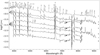 |
Fig. 1. Low resolution optical spectral evolution of optically thick phase of T Pyx from 2011 April 15 to 2011 April 22. The spectra are dominated by P Cygni profiles. The identified lines and time since discovery in days (numbers to the right) are marked. The P Cygni absorption components become sharper and deeper as the system evolves. |
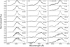 |
Fig. 2. High resolution spectral (R = 27 000) evolution of T Pyx from 2011 April 16 to 2011 June 10. Evolution of Hα, Hβ, and O I (8446 Å) line profiles are shown. We note the variation in the velocity of the lines as the system evolves. There is a decrease in velocity from day 2.31 to 12.32 and then an increase up to ∼2000 km s−1 until day 57.29. |
Fe II multiplets (Fig. 3) are the most dominant non-Balmer lines as the system evolves to its optical maximum, and during the early decline (days 14.31–68.28). The O I (8446 Å) line, which was an emission line until the previous phase, develops a P Cygni profile from day 22.29 to 28.27 (around the optical maximum). The Fe II multiplets, Balmer, and O I lines that have P Cygni profiles slowly evolve into emission lines towards the end of this phase. The Hα line becomes broader with a velocity up to ∼2000 km s−1 with a rounded peak profile near the optical maximum. The full width half maximum (FWHM) of the lines increases from ∼1000 to ∼2000 km s−1 during day 14.31 to 68.28. From day 42.30 to 68.28, the presence of [N II] (5755 Å) and N II lines is clearly seen. The emission component of N II (5679 Å) P Cygni profile, which is weak on ∼day 14, becomes stronger by ∼day 42.
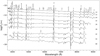 |
Fig. 3. Evolution of the spectra as the T Pyx system passes through its optical maximum and early decline phase from 2011 April 28 to 2011 June 21. The significant development in this phase is the presence and slow evolution of Fe II multiplet profiles from P Cygni to emission lines. The identified lines and time since discovery in days (numbers to the right) are marked. |
The nebular phase (day 223.66–648.80) is marked by dominant, broad [O III] 4959 and 5007 Å lines (Fig. 4). The [N II] line develops a double-peaked profile with wing-like structures on either side, which is similar to the [O III] and the Balmer lines. Other forbidden lines seen are the [Fe VII] (5158, 5276 and 6087 Å), [Fe X] (6375 Å), [O II] (7330 Å), [C III] + [O III] (Blend 4364 Å with H I), and [Ne III] (3869 and 3968 Å) lines. The intensity of the [N II] and [Fe VII] lines slowly decreases and [N II] disappears by day 1064. By day 1064, all the nebular lines disappear, except for the [O III] 4959, 5007 Å lines. The intensity of [O III] lines reduced during the nova’s decline to late post-outburst phase during day 1064.39–2415.62 (Fig. 5).
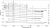 |
Fig. 4. Evolution of the spectra during nebular phase of T Pyx from 2011 Nov. 23 to 2013 Jan. 21. The emission line profiles are double-peaked with wing-like structures on both the sides. Presence of the forbidden lines can clearly be seen during this phase. The identified lines and time since discovery in days (numbers to the right) are marked. |
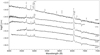 |
Fig. 5. Evolution of the spectra during the late post-outburst phase of T Pyx from 2014 Mar. 13 to 2017 Nov. 23. As the system evolves, the lines develop into narrow emission ones from broader profiles. The [O III] lines are blue-shifted by ∼780 km s−1 beyond day 1721 and the [N II] 6874 Å line can clearly be seen in this phase. The identified lines and time since discovery in days (numbers to the right) are marked. |
Strong helium emission lines are seen during this phase. The [O III] lines show a blueshift by ∼780 km s−1 beyond day 1721, which is not seen in the hydrogen and helium emission lines. This could be due to the fact that while the [O III] lines arise in the fading nova ejecta, the hydrogen and helium lines arise in the accretion disc.
3.2. Polarization of the ejecta
The degree of polarization and position angle values estimated for T Pyx during its 2011 outburst are given in Table 4. During the initial rise phase, the degree of polarization is found to increase in all bands until day 4–5, and decrease subsequently. For example, the degree of polarization in the V increased from a value of 0.69% on day 1.36 to 1.27% on day 5.35, and decreased to 0.37% by day 8.34. The degree of polarization was found to have increased from the estimate on day 8.34 during the next set of observations on days 28.34 and 29.33, with a rising trend. The position angle was found to be 112 ° ±18° during the entire period of observation.
Polarimetric observations of T Pyx during its 2011 outburst.
Intrinsic polarization of the ejecta was detected by Eggen et al. (1967) during the 1967 outburst, which was found to vary with time. Polarization values of T Pyx during its 2011 outburst have been compared with those reported for the 1967 outburst during days 1.96–44.02. In Fig. 6, the epochs of polarization observations made during the two outbursts are highlighted. The variability in degree of polarization values in different filters for both the outbursts is shown in Fig. 7. An identical pattern in the variation of degree of polarization is observed in both the outbursts; there is an initial rise in the values followed by a decrease in the early pre-maximum phase, followed by an increase in the degree of polarization during the optical maximum. While the trend is similar, the degree of polarization is lower in the 2011 outburst compared with the 1967 outburst. The maximum values of polarization in the B filter and V filter are 2.3% and 2.32% respectively for the 1967 outburst, while for the 2011 outburst it is 1.25% and 1.27% in the B and V filters, respectively. Position angles observed during the 2011 outburst are consistent with those of the 1967 outburst (Fig. 7). Although both the 1967 and 2011 values are uncorrected for interstellar polarization, the very similar behaviour during both epochs indicates intrinsic polarization.
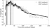 |
Fig. 6. Light curve for T Pyx during its 1967 and 2011 eruptions. The black squares and grey circles correspond to the 2011 and 1967 eruptions, respectively. The black and grey dashed lines correspond to the polarization epochs during the 2011 and 1967 eruptions, respectively. |
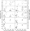 |
Fig. 7. Variability in the degree of polarization and position angle for 2011 and 1967 outbursts. The squares and circles correspond to the 2011 and 1967 outbursts, respectively. |
4. Photo-ionization analysis
The evolution of the emission spectrum during and after the 2011 outburst was modelled to understand the physical conditions and the variation in the physical conditions as the system evolves. The photo-ionization code CLOUDY, C17.00 (Ferland et al. 2017) was used to model the evolution. CLOUDY has been applied to determine the physical characteristics and elemental abundances of novae in a few previous studies (Schwarz et al. 2001, 2007a,b; Schwarz 2002; Vanlandingham et al. 2005; Helton et al. 2010; Das & Mondal 2015; Mondal et al. 2018; Raj et al. 2018). Spectra obtained at epochs of day 68, 224, 252, 336, and 1064 corresponding to different phases were modelled. The modelled synthetic spectrum was compared with the observed spectrum and parameters such as elemental abundances, density, source luminosity, and source temperature were obtained. These parameters were used as inputs to model the 3D ionization structure of the ejecta.
To obtain the 3D ionization structure of the ejecta, pyCloudy (Morisset 2013) was used. Modelling the 3D ionization structure of the ejecta would reveal the spatial distribution of elements at different epochs and also their evolution with time. This would result in understanding the origin of different lines at different phases. This work is an attempt to understand the spatial origin of the ionization lines, which is not well understood. The pyCloudy is a pseudo-3D code that uses the CLOUDY 1D (Ferland et al. 2017) photo-ionization code and Python library to analyse the models. The 3D CLOUDY model can be obtained by generating 1D CLOUDY fits corresponding to different angles and interpolating these runs (radial radiation) to form a 3D coordinate cube. The Python library includes routines that enable tasks such as visualizing the models and integrating masses and fluxes. The photo-ionization models used in pyCloudy are 1D codes and they do not deal with the effect of the diffuse radiation field entirely; also Python codes are limited by symmetry, hence it is referred to as pseudo-3D and not complete 3D code. Using photo-ionization modelling is usually a good enough approximation to study physical conditions in novae. Full 3D codes that use Monte Carlo methods and hydrodynamic calculations will be considered at a later point in a future paper.
Many parameters are used in CLOUDY to define the initial physical conditions of the source and the ejected shell. These parameters include the shape and intensity of the external radiation field striking a cloud, the chemical composition of the gas, and the geometry of the gas, including its radial extent and dependence of density on radius. CLOUDY generates a predicted spectrum using these input parameters by solving the equations of thermal and statistical equilibrium from non-local thermodynamic equilibrium (NLTE), illuminated gas clouds. The density, radii, geometry, distance, covering factor, filling factor, and elemental abundances define the physical conditions of the shell. The density of the shell is defined by hydrogen density. The radial variation of hydrogen density, n(r), and filling factor, f(r), are
 (1)
(1)
where r0 is the inner radius, and α and β are exponents of power laws. Here, α = −3 for a shell undergoing ballistic expansion, and the filling factor power-law exponent is β = 0, similar to previous studies (Schwarz 2002; Vanlandingham et al. 2005; Helton et al. 2010; Das & Mondal 2015).
In the 1D model, the geometry of the shell was assumed to be a spherically symmetric, expanding one illuminated by the central source. Many spectra were generated to obtain the best fit for each epoch by varying free parameters like hydrogen density, effective blackbody temperature, and abundances of the elements that were seen in the observed spectrum, while the remaining elements were fixed at the solar values. The ejecta was assumed to be made of more than one density region in order to fit all the ionized lines. A covering factor was set in all the regions such that the sum was always equal to one. All parameters, except for hydrogen density and the covering factor, were kept constant in all the regions, so that the number of free parameters from the regions was reduced. Modelled line ratios were obtained by adding line ratios of each region after multiplying by its covering factor. The inner and outer radii of the ejected shell were set by the time of observation, and minimum and maximum expansion velocities obtained using full width at half maximum of all the emission lines, similar to the studies by Schwarz (2002), Schwarz et al. (2007b), Helton et al. (2010), and Mondal et al. (2018).
The best-fit model was obtained by calculating χ2 and reduced χ2:
 (2)
(2)
where Mi and Oi are the modelled and observed line ratios, σi is the error in observed flux ratio, n is the number of observed lines, np is the number of free parameters, and ν = n − np are the degrees of freedom.
The ejected mass was determined using the relation (e.g. Schwarz et al. 2001; Schwarz 2002; Das & Mondal 2015)
 (3)
(3)
The ejected mass was calculated for all the regions, then multiplied by the corresponding covering factors and added to obtain the final value. The abundance values and other parameters are obtained from the model. The abundance solutions are sensitive to changing opacity and physical conditions of the ejecta such as temperature.
The initial structure of the cloud for 3D modelling was assumed to be an axisymmetric spheroid. The input parameters for this central source were defined using the best-fit 1D CLOUDY results obtained for each epoch. Parameters adopted were effective blackbody temperature, abundance values, density, filling factor, and inner and outer radii. Six 1D CLOUDY runs at different radial directions were used to build this 3D cube. All the 1D models with their respective radial direction are inclined to the equatorial plane at a specified angle with the inner and outer radii. In every 1D run, the elemental abundances and luminosity were kept constant while temperature, inner and outer radii, and density were varied. In every radial direction (1D run), the emissivity values of every element present in the observed spectrum were interpolated to obtain the 3D emissivity values for every element. The dimension of the 3D cube is 301 × 301 × 301.
4.1. Early decline phase
For this phase, the spectrum of day 68 was modelled. The central ionizing source was set to be at effective temperature 105 K and luminosity 1037 erg s−1. Three different regions were used to obtain the synthetic spectrum: a diffused region with density 4.46 × 108 cm−3 to fit most of the lines like helium, C III, and [N II]; Fe II lines were fit dominantly by a clumpy region with a higher density, 5.62 × 108 cm−3; and N II recombination lines were fit using a region with lower temperature, 3 × 10⁴ K, and a higher density, 5.62 × 108 cm−3.
The relative fluxes of the observed lines, best-fit modelled lines, and corresponding χ2 values are given in Table 5, and the values of best-fit parameters are given in Table 6. The estimated abundance values show that nitrogen and helium abundances are more than solar, while iron, calcium, and carbon abundance values are solar. The best-fit modelled spectrum (dashed line) with the corresponding observed optical spectrum (continuous line) are as shown in Fig. 8. Absorption components of the P Cygni profiles are not modelled here because of the limitations of the code. The best-fit parameters obtained for this epoch are accurate to 65–70% only.
Best-fit CLOUDY model parameters for day 68.
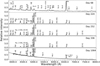 |
Fig. 8. Best-fit CLOUDY model spectra (dashed line) plotted over the observed spectra (continuous line) of T Pyx obtained on day 68, 224, 252, 336, and 1064. The spectra are normalized to Hβ. The identified lines and time since discovery in days (numbers to the right) are marked. |
4.2. Nebular phase
Three epochs, day 224, 252, and 336, were modelled to understand the evolution during the nebular phase. Two regions were used to model the observed spectrum. Most of the lines were fitted by the clump component, except a few forbidden lines like [N II] (5755 Å), [O III] (4959 and 5007 Å), and [Ne III] (3869 and 3968 Å). In order to fit all the lines, a diffuse region (low density) was used, covering 20% of the volume. The central ionizing source was set to be at an effective temperature ∼105 K and luminosity ∼1037 erg s−1. The clump hydrogen density is in the range of (5.6–7.9) × 107 cm−3 and diffuse hydrogen density (1.8–3.2) × 107 cm−3. The relative fluxes of the observed lines, best-fit model predicted lines, and corresponding χ2 values are given in Table 7. The values of best-fit parameters obtained from the model are given in Table 8. The estimated abundance values show that helium, nitrogen, oxygen, and neon are over-abundant compared to solar, while iron and carbon have the solar abundance values. On day 252, nitrogen and helium abundance values are more than that of day 224 and 336. Oxygen abundance values continue to be above the solar values in all the epochs. The best-fit modelled spectra for all the epochs are shown in Fig. 8 together with the corresponding observed spectra.
Observed and best-fit CLOUDY model line flux values for epochs of nebular and late post-outburst phase.
Best-fit CLOUDY model parameters during the nebular phase.
The geometry of the ionized structure during this phase was found to be a bipolar conical one with equatorial rings (Fig. 9). The [O III] emission is dominant in the outermost regions of the cones and equatorial rings. The emissivity increases with time while the structure remains the same (Fig. 10). The nitrogen lines are present in the innermost regions of the equatorial rings and cones. The He II (4686 Å) line is present in the innermost regions of the cones, while hydrogen lines are present in the innermost regions of the equatorial rings. No significant change is seen in the emissivity of these lines.
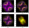 |
Fig. 9. Evolution of the geometry of ejecta on day 224 (top left panel), 252 (top right panel), 336 (bottom left panel), and 1064 (bottom right panel). We note the formation of multiple equatorial rings and also the spatial distribution of the ionized lines as the system evolves. Here, a: [O III] λ5007, b: [O III] λ4959, c: Hα, d: Hβ, e: N III λ4638, f: [N II] λ5755, g: He II λ4686. Only dominant lines are marked. Here, 1 unit of x and y position correspond to x224 = 6.3 × 1012 cm, x252 = 1.41 × 1013 cm, x336 = 2.09 × 1013 cm, and x1064 = 1.66 × 1012 cm. |
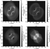 |
Fig. 10. Evolution of [O III] (4959 and 5007 Å lines) on day 224 (top left panel), 252 (top right panel), 336 (bottom left panel), and 1064 (bottom right panel). We note the increase in intensity from day 224 to day 336 and then the drop in intensity on day 1064. Here, one unit of x and y position corresponds to x224 = 6.3 × 1012 cm, x252 = 1.41 × 1013 cm, x336 = 2.09 × 1013 cm, and x1064 = 3.31 × 1011 cm. |
4.3. Late post-outburst phase
During this phase, the spectrum obtained on day 1064 was modelled. The observed spectrum is dominated by hydrogen, helium, and [O III] lines as discussed in Sect. 3.1. A two-component model was considered in order to generate the model spectrum. One component had an ionizing source of luminosity 1035 erg s−1, and disc with density 2 × 109 cm−3 at T = 7.5 × 10⁴ K and cylindrical semi height, 104 cm. The helium and hydrogen lines were dominantly fit by this component. The other component had a similar ionizing source luminosity and lesser density region, 106 cm−3 at T = 9.5 × 10⁴ K. The [O III] and nitrogen lines were fit using this component. The radius, luminosity, and density were calculated by adopting the values of mass of the white dwarf (WD), accretion rate, period, and binary separation from Patterson et al. (2017) and Selvelli et al. (2008). The modelled spectrum was obtained by adding the values generated by the above components (Fig. 8). Best-fit parameters were obtained for these values (Table 9). The estimated abundance values of helium, nitrogen, and oxygen were found to be more than those of the solar abundance values.
Best-fit CLOUDY model parameters for the late post-outburst phase spectrum.
The ionized structures of different lines obtained in this phase have distinct spatial locations unlike previous epochs. The overall geometry of the ionized ejecta is dominantly divided into a nitrogen zone, an oxygen zone, and a helium–hydrogen zone (from outer to inner regions) as shown in Fig. 9. The conical structures appear to have evolved compared to the previous epochs. The outermost regions and the cones are of nitrogen lines and the next inner regions are of [O III] lines indicating that they are coming from a shell ejected by the system. The helium lines are coming from the region of a radius of about 7.4 × 109 cm. If the accretion rate suggested by Godon et al. (2018) is considered, then this radius value would correspond to that of the outermost regions of accretion disc. This suggests that helium lines predominantly come from the accretion disc.
4.4. Results
The best-fit model obtained for day 68 was used to fit only the emission components. The P Cygni profiles and O I (7774 Å) line were not modelled due to the limitations of the code. The N II (5679 Å) line has a high χ2 value, a broad emission component, and a narrow absorption component. The He II (4686 Å) line has higher χ2 values and hence contributes more to the total χ2. In the late post-outburst phase, the [O III] and He I (7065 Å) lines have higher χ2 values. Though the reduced χ2 values suggest that the generated spectrum matches the observed spectrum well, the above contributions from different lines might hinder the calculated abundance values. The higher χ2 values are as a consequence of blending of the lines. The [Fe VII] (6087 Å) line has a higher χ2 value on a few days. It is a coronal line possibly excited by shock interaction, hence resulting in a higher χ2 value. The variation of the best-fit parameters during the system’s evolution is given in Fig. 11.
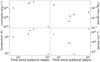 |
Fig. 11. Variation of best-fit parameters obtained from CLOUDY such as luminosity, effective temperature, density, and ejected shell mass are shown. |
The estimate of the ejected mass, averaged over all epochs, is 7.03 × 10⁻⁶ M⊙. This value is similar to that obtained by Shore et al. (2013). Best-fit model parameters suggest the presence of a hot WD source with a roughly constant luminosity of 1037 erg s−1. Helium and nitrogen abundance values are above solar values in all the phases, whereas neon is more only during nebular phase. Oxygen abundance is also found to be more than solar, while the iron and calcium abundances are nearly solar. Though the distance to T Pyx used for analysis is 4.8 kpc, the results were also verified for the distance given by Gaia of ∼3 kpc. The 1D CLOUDY results do not vary as relative intensity is considered for the calculations.
The modelled structure of the ionized ejecta shows that the evolution of the ejecta is consistent with the line profiles observed. The variation in the spatial distribution of the elements as the physical conditions change from one epoch to another is consistent with the observed spectra. The best-fit modelled velocity profile (dashed line) with the corresponding observed optical velocity profile (continuous line) of Hα and [O III] λ5007 are as shown in Fig. 12. The best-fit modelled profiles are symmetric here as the initial geometry was assumed to be spherically symmetric (refer to the introduction of Sect. 4). The inner and outer cone angles found using this method are consistent with that estimated by Shore et al. (2013). The inner conical angles lie in the range of 21.08°–77.86° while the outer conical angles varied from 49.89° to 87.75°. The value of the inclination angle of the ejecta axis to the line of sight was found to be 14.75 ° ±0.65°. This value is consistent with that of the values reported by Patterson et al. (1998), Chesneau et al. (2011), and Shore et al. (2013).
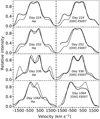 |
Fig. 12. Best-fit pyCloudy model velocity profile (dashed line) at i ∼ 14.75° plotted over the observed profile of Hα and [O III] λ5007 (continuous line) of T Pyx obtained on day 224, 252, 336, and 1064. |
5. Discussion
The optical spectral evolution of T Pyx from its 2011 outburst discovery to the subsequent quiescent phase has been discussed in this paper. This outburst is similar to the previous ones, but many variations in the physical conditions at different epochs that are relevant to the system, including the presence of distinct ionization lines and the evolution of line profiles, were possible to study because of good coverage.
Spectral lines observed have P Cygni profiles with sharp and deep narrow absorption components and narrow emission components until the early decline phase. These slowly evolve into broader double-peaked emission lines with wing-like structures during the nebular phase. Finally, these wing-like structures (left and right) disappear resulting in sharp and narrow emission lines in the late post-outburst phase. There is a decrease in ejecta velocity from ∼2500 km s−1 to ∼1000 km s−1 during the initial pre-maximum phase from t = 1.28 to 12.32, and then velocity increases up to ∼2000 km s−1 on its way to optical maximum and the decline phase. Weak N II lines from day 14.31 are seen, which become stronger towards the decline phase. The transition of the system from He/N to Fe II type occurs when it is rising to its optical maximum. The [O III] 4959 and 5007 Å lines appear to be blue-shifted in the late post-outburst phase while other lines are not shifted. This might be due to the motion of the doubly ionized oxygen shell towards us.
Nearly solar abundances are found for iron and calcium seen during the optically thick Fe II phase, while elements like helium, nitrogen, oxygen, and neon are more than solar during both the Fe II and nebular (He/N) phases. The ejected mass during the decline phase at t = 68 days is estimated to be 2.74 × 10⁻⁵ M⊙. During the nebular phase, it is of the order of 10−6 M⊙. Based on the observed period change before and after the 2011 eruption, Patterson et al. (2017) estimated the ejected mass to be ≥3 × 10⁻⁵ M⊙, while Nelson et al. (2014) estimated the ejected mass as (1 − 30)×10−5 M⊙ using the high peak flux densities in the radio emission. Based on the late turn-on time for the SSS phase, Chomiuk et al. (2014) suggested a large ejecta mass of ⪆10−5 M⊙. Using high resolution optical spectroscopic observations obtained on day 180 and 360, Shore et al. (2013) estimated the ejected mass to be Mej = 2 × 10⁻⁶ M⊙, similar to the values reported here for the nebular phase. The ejected mass estimates for other recurrent novae are ∼10−7 − 10−6 M⊙, while the estimates for classical novae are in general higher, at ∼10−5 − 10−4 M⊙. The ejected mass obtained for the T Pyx system in the early phase (day 68) is similar to classical novae, while for the nebular phase the ejected mass values are similar to recurrent novae. Using accretion disc models, Godon et al. (2018) estimate a mass accretion rate of 10−6 M⊙yr−1 for a distance of 4.8 kpc, or a rate of 10−7 M⊙yr−1 for the Gaia distance estimate of ∼3.3 kpc, for a white dwarf mass of 1.35 M⊙. This indicates the mass accumulated between the 1967 and 2011 outbursts is lower than the ejected mass, for an ejecta mass of ≳10−5 M⊙.
The geometry of the ionized structure of the ejecta is a bipolar conical one with equatorial rings. We note that [O III] and nitrogen lines mainly come from the outer regions, and hydrogen lines from the inner regions. As the shell evolves, expansion of equatorial rings can clearly be seen in the nebular phase. In the late post-outburst phase, a complex structure of [O III] and nitrogen is formed with an inner helium and hydrogen structure, most likely from the accretion disc. From the study of Chesneau et al. (2011), it is known that the system is oriented nearly face-on and it is bipolar. Hence, the outer regions (especially [O III]) are moving away from the central system towards us (nearly face-on) resulting in the blue-shifted [O III] lines from day 1721.
Polarimetric studies of novae have revealed the presence of linear polarization in systems like U Sco (Anupama et al. 2013), V339 Del (Shakhovskoy et al. 2017), RS Oph (Cropper 1990), and also during the 1967 outburst of T Pyx (Eggen et al. 1967). The intrinsic linear polarization during the SSS phase in U Sco was explained as being due to scattering from discs and jets. In the case of V339 Del, variability in the polarization parameters was observed, and interpreted as being due to a non-spherical diffuse shell, with a geometry that was more likely bipolar than disc-shaped. In RS Oph (1985 outburst), the intrinsic linear polarization was suggested as being due to electron scattering in the aspherically expanding nova ejecta. Linear polarized emission has been observed from the T Pyx system in the BVRI bands during the 1967 as well as the 2011 outbursts. The observed polarization in T Pyx is variable, with a very similar trend during both outbursts. Although not corrected for interstellar polarization, the similar trend indicates the polarization to be intrinsic, which can be suggested as being due to a) asymmetry of the ejecta at the time of outburst, and/or b) the presence of silicate grains, as suggested by Svatoš (1983) for the 1967 eruption. IR observations of T Pyx during the 2011 outburst suggest the presence of pre-outburst dust in the system with a mass of ∼10−5 M⊙ (Evans et al. 2012). Asymmetry in the system at the time of outburst can be due to the interaction of the initial ejecta with circumstellar material, also resulting in the decrease in velocity as observed in the spectral data until day 12.32. Coincidentally, there was a marginal detection of hard X-rays during days 14–20, which has been attributed by Chomiuk et al. (2014) to an interaction of the nova ejecta with a pre-existing circumbinary material. Such an interaction has also been shown to result in equatorial rings or regions (Soker 2015; Bode et al. 2007; Livio et al. 1990; Lloyd et al. 1997) similar to those seen in the models presented here.
6. Summary
Evolution of the optical spectrum of the 2011 outburst of the recurrent nova T Pyxidis is presented here based on an extensive dataset over the period day 1.28–2415.62 since discovery of the outburst. Also presented is the polarisation property during the early phase of the outburst. Physical conditions in the outburst ejecta, and the geometry of the ionized structure of the nova ejecta are modelled for a few epochs using the photo-ionization code, CLOUDY in 1D and pyCloudy in 3D. The main results of the analyses are summarised here.
-
The evolution is similar to that of the previous outbursts.
-
The emission lines during the early pre-maximum phase have P Cygni profiles with deep and narrow absorption components and sharp emission peaks, with the ejecta velocity decreasing from 2500 km s−1 to 1000 km s−1 until ∼day 12.
-
The rise to optical maximum and early decline phase have P Cygni profiles with round peaked emission components and slowly fading absorption components, with the ejecta velocity increasing from 1000 km s−1 to 2000 km s−1 until ∼day 68.
-
The emission lines in the nebular phase are broad and double peaked with wing-like structures on both the sides. The emission lines in the late post-outburst phase are narrow, and [O III] lines show a blueshift by ∼780 km s−1 beyond day 1721.
-
The photo-ionization code CLOUDY was used to model the spectra of five epochs, and the modelled spectra match the observational spectra fairly well. From these results, elemental abundances, temperature, luminosity of the WD, and density of the ejecta were estimated at all the epochs. Helium, nitrogen, oxygen, and neon were found to be over abundant compared to solar values.
-
The ejected mass during the Fe II phase of the system is estimated to be 2.74 × 10⁻⁵ M⊙ while during the nebular phase it is ∼2 × 10⁻⁶ M⊙.
-
The pseudo 3D code pyCLOUDY was used to model the ionized structure of ejecta for four epochs. The geometry was found to be bipolar conical with equatorial rings, with an inclination angle of 14.75 ° ±0.65°. At the late post-outburst phase, it appears that the [O III] lines come from an expanding ejecta while the hydrogen and helium lines are from the accretion disc.
-
A variable, intrinsic linear polarization was observed, which could be either due to asymmetry in the initial ejecta and/or the presence of silicate grains.
IRAF is distributed by the National Optical Astronomy Observatories, which are operated by the Association of Universities for Research in Astronomy, Inc., under cooperative agreement with the National Science Foundation.
Acknowledgments
We thank the referee for a critical reading of the manuscript. We thank all the observers of the 2 m HCT at the IAO, 2 m IGO telescope at the IGO and also the 2.3 m VBT at the VBO for accommodating some time for ToO observations. We thank the respective TACs for the allocation of time and support during ToO and regular observations. The IAO and VBO are operated by the Indian Institute of Astrophysics, Bangalore and the IGO by Inter-University Centre for Astronomy and Astrophysics, Pune. We thank Mr. Avinash Singh for the aperture photometry code https://github.com/sPaMFouR/RedPipe that was used for polarization data reduction. We acknowledge with thanks the variable star observations from the AAVSO International Database contributed by observers worldwide and used in this research.
References
- Anupama, G. C. 2008, in RS Ophiuchi (2006) and the Recurrent Nova Phenomenon, eds. A. Evans, M. F. Bode, T. J. O’Brien, & M. J. Darnley, ASP Conf. Ser., 401, 31 [Google Scholar]
- Anupama, G. C., Kamath, U. S., Ramaprakash, A. N., et al. 2013, A&A, 559, A121 [NASA ADS] [CrossRef] [EDP Sciences] [Google Scholar]
- Bode, M. F., Harman, D. J., O’Brien, T. J., et al. 2007, ApJ, 665, L63 [NASA ADS] [CrossRef] [Google Scholar]
- Chesneau, O., Meilland, A., Banerjee, D. P. K., et al. 2011, A&A, 534, L11 [NASA ADS] [CrossRef] [EDP Sciences] [Google Scholar]
- Chomiuk, L., Nelson, T., Mukai, K., et al. 2014, ApJ, 788, 130 [NASA ADS] [CrossRef] [Google Scholar]
- Clarke, D., Smith, R. A., & Yudin, R. V. 1998, A&A, 336, 604 [NASA ADS] [Google Scholar]
- Cropper, M. 1990, MNRAS, 243, 144 [NASA ADS] [CrossRef] [Google Scholar]
- Das, R., & Mondal, A. 2015, New Astron., 39, 19 [NASA ADS] [CrossRef] [Google Scholar]
- De Gennaro Aquino, I., Shore, S. N., Schwarz, G. J., et al. 2014, A&A, 562, A28 [NASA ADS] [CrossRef] [EDP Sciences] [Google Scholar]
- Duerbeck, H. W. 1987, Space Sci. Rev., 45, 1 [NASA ADS] [CrossRef] [Google Scholar]
- Duerbeck, H. W., & Seitter, W. C. 1979, The Messenger, 17, 1 [NASA ADS] [Google Scholar]
- Eggen, O. J., Mathewson, D. S., & Serkowski, K. 1967, Nature, 213, 1216 [NASA ADS] [CrossRef] [Google Scholar]
- Evans, A., Gehrz, R. D., Helton, L. A., et al. 2012, MNRAS, 424, L69 [NASA ADS] [CrossRef] [Google Scholar]
- Ferland, G. J., Chatzikos, M., Guzmán, F., et al. 2017, Rev. Mex. Astron. Astrofis., 53, 385 [NASA ADS] [Google Scholar]
- Godon, P., Sion, E., Williams, R., & Starrfield, S. 2018, AJ, 862, 89 [CrossRef] [Google Scholar]
- Goswami, A., & Karinkuzhi, D. 2013, A&A, 549, A68 [NASA ADS] [CrossRef] [EDP Sciences] [Google Scholar]
- Goswami, A., Kartha, S. S., & Sen, A. K. 2010, ApJ, 722, L90 [NASA ADS] [CrossRef] [Google Scholar]
- Helton, L. A., Woodward, C. E., Walter, F. M., et al. 2010, AJ, 140, 1347 [NASA ADS] [CrossRef] [Google Scholar]
- Izzo, L., Ederoclite, A., Della Valle, M., et al. 2012, Mem. Soc. Astron. It., 83, 830 [NASA ADS] [Google Scholar]
- Joshi, V., Banerjee, D. P. K., & Ashok, N. M. 2014, MNRAS, 443, 559 [NASA ADS] [CrossRef] [Google Scholar]
- Livio, M., Shankar, A., Burkert, A., & Truran, J. W. 1990, ApJ, 356, 250 [NASA ADS] [CrossRef] [Google Scholar]
- Lloyd, H. M., O’Brien, T. J., & Bode, M. F. 1997, MNRAS, 284, 137 [NASA ADS] [CrossRef] [Google Scholar]
- Mondal, A., Anupama, G. C., Kamath, U. S., et al. 2018, MNRAS, 474, 4211 [NASA ADS] [CrossRef] [Google Scholar]
- Morisset, C. 2013, Astrophysics Source Code Library [record ascl:1304.020] [Google Scholar]
- Nelson, T., Chomiuk, L., Roy, N., et al. 2014, ApJ, 785, 78 [NASA ADS] [CrossRef] [Google Scholar]
- Patterson, J., Kemp, J., Shambrook, A., et al. 1998, PASP, 110, 380 [NASA ADS] [CrossRef] [Google Scholar]
- Patterson, J., Oksanen, A., Kemp, J., et al. 2017, MNRAS, 466, 581 [NASA ADS] [CrossRef] [Google Scholar]
- Raj, A., Pavana, M., Kamath, U. S., Anupama, G. C., & Walter, F. M. 2018, Acta Astron., 68, 79 [NASA ADS] [Google Scholar]
- Ramaprakash, A. N., Gupta, R., Sen, A. K., & Tandon, S. N. 1998, A&AS, 128, 369 [NASA ADS] [CrossRef] [EDP Sciences] [Google Scholar]
- Schaefer, B. E. 2018, MNRAS, 481, 3033 [NASA ADS] [CrossRef] [Google Scholar]
- Schaefer, B. E., Landolt, A. U., Linnolt, M., et al. 2013, ApJ, 773, 55 [NASA ADS] [CrossRef] [Google Scholar]
- Schaefer, B. E., Pagnotta, A., & Shara, M. M. 2010, ApJ, 708, 381 [NASA ADS] [CrossRef] [Google Scholar]
- Schwarz, G. J. 2002, ApJ, 577, 940 [NASA ADS] [CrossRef] [Google Scholar]
- Schwarz, G. J., Shore, S. N., Starrfield, S., et al. 2001, MNRAS, 320, 103 [NASA ADS] [CrossRef] [Google Scholar]
- Schwarz, G. J., Shore, S. N., Starrfield, S., & Vanlandingham, K. M. 2007a, ApJ, 657, 453 [NASA ADS] [CrossRef] [Google Scholar]
- Schwarz, G. J., Woodward, C. E., Bode, M. F., et al. 2007b, AJ, 134, 516 [NASA ADS] [CrossRef] [Google Scholar]
- Selvelli, P., Cassatella, A., Gilmozzi, R., & González-Riestra, R. 2008, A&A, 492, 787 [NASA ADS] [CrossRef] [EDP Sciences] [Google Scholar]
- Serkowski, K. 1974, in Planets, Stars and Nebulae Studied with Photopolarimetry, ed. T. Gehrels (Tucson: Univ. of Arizona Press), 135 [Google Scholar]
- Shakhovskoy, D. N., Antonyuk, K. A., & Belan, S. P. 2017, Astrophysics, 60, 19 [NASA ADS] [CrossRef] [Google Scholar]
- Shara, M. M., Moffat, A. F. J., Williams, R. E., & Cohen, J. G. 1989, ApJ, 337, 720 [NASA ADS] [CrossRef] [Google Scholar]
- Shara, M. M., Zurek, D. R., Williams, R. E., et al. 1997, AJ, 114, 258 [NASA ADS] [CrossRef] [Google Scholar]
- Shore, S. N., Schwarz, G. J., De Gennaro Aquino, I., et al. 2013, A&A, 549, A140 [NASA ADS] [CrossRef] [EDP Sciences] [Google Scholar]
- Soker, N. 2015, ApJ, 800, 114 [NASA ADS] [CrossRef] [Google Scholar]
- Sokoloski, J. L., Crotts, A. P. S., Lawrence, S., & Uthas, H. 2013, ApJ, 770, L33 [NASA ADS] [CrossRef] [Google Scholar]
- Surina, F., Hounsell, R. A., Bode, M. F., et al. 2014, AJ, 147, 107 [NASA ADS] [CrossRef] [Google Scholar]
- Svatoš, J. 1983, Astrophys. Space Sci., 93, 347 [NASA ADS] [CrossRef] [Google Scholar]
- Toraskar, J., Mac Low, M.-M., Shara, M. M., & Zurek, D. R. 2013, ApJ, 768, 48 [NASA ADS] [CrossRef] [Google Scholar]
- Vanlandingham, K. M., Schwarz, G. J., Shore, S. N., Starrfield, S., & Wagner, R. M. 2005, ApJ, 624, 914 [NASA ADS] [CrossRef] [Google Scholar]
All Tables
Observed and best-fit CLOUDY model line flux values for epochs of nebular and late post-outburst phase.
All Figures
|
Fig. 1. Low resolution optical spectral evolution of optically thick phase of T Pyx from 2011 April 15 to 2011 April 22. The spectra are dominated by P Cygni profiles. The identified lines and time since discovery in days (numbers to the right) are marked. The P Cygni absorption components become sharper and deeper as the system evolves. |
| In the text | |
|
Fig. 2. High resolution spectral (R = 27 000) evolution of T Pyx from 2011 April 16 to 2011 June 10. Evolution of Hα, Hβ, and O I (8446 Å) line profiles are shown. We note the variation in the velocity of the lines as the system evolves. There is a decrease in velocity from day 2.31 to 12.32 and then an increase up to ∼2000 km s−1 until day 57.29. |
| In the text | |
|
Fig. 3. Evolution of the spectra as the T Pyx system passes through its optical maximum and early decline phase from 2011 April 28 to 2011 June 21. The significant development in this phase is the presence and slow evolution of Fe II multiplet profiles from P Cygni to emission lines. The identified lines and time since discovery in days (numbers to the right) are marked. |
| In the text | |
|
Fig. 4. Evolution of the spectra during nebular phase of T Pyx from 2011 Nov. 23 to 2013 Jan. 21. The emission line profiles are double-peaked with wing-like structures on both the sides. Presence of the forbidden lines can clearly be seen during this phase. The identified lines and time since discovery in days (numbers to the right) are marked. |
| In the text | |
|
Fig. 5. Evolution of the spectra during the late post-outburst phase of T Pyx from 2014 Mar. 13 to 2017 Nov. 23. As the system evolves, the lines develop into narrow emission ones from broader profiles. The [O III] lines are blue-shifted by ∼780 km s−1 beyond day 1721 and the [N II] 6874 Å line can clearly be seen in this phase. The identified lines and time since discovery in days (numbers to the right) are marked. |
| In the text | |
|
Fig. 6. Light curve for T Pyx during its 1967 and 2011 eruptions. The black squares and grey circles correspond to the 2011 and 1967 eruptions, respectively. The black and grey dashed lines correspond to the polarization epochs during the 2011 and 1967 eruptions, respectively. |
| In the text | |
|
Fig. 7. Variability in the degree of polarization and position angle for 2011 and 1967 outbursts. The squares and circles correspond to the 2011 and 1967 outbursts, respectively. |
| In the text | |
|
Fig. 8. Best-fit CLOUDY model spectra (dashed line) plotted over the observed spectra (continuous line) of T Pyx obtained on day 68, 224, 252, 336, and 1064. The spectra are normalized to Hβ. The identified lines and time since discovery in days (numbers to the right) are marked. |
| In the text | |
|
Fig. 9. Evolution of the geometry of ejecta on day 224 (top left panel), 252 (top right panel), 336 (bottom left panel), and 1064 (bottom right panel). We note the formation of multiple equatorial rings and also the spatial distribution of the ionized lines as the system evolves. Here, a: [O III] λ5007, b: [O III] λ4959, c: Hα, d: Hβ, e: N III λ4638, f: [N II] λ5755, g: He II λ4686. Only dominant lines are marked. Here, 1 unit of x and y position correspond to x224 = 6.3 × 1012 cm, x252 = 1.41 × 1013 cm, x336 = 2.09 × 1013 cm, and x1064 = 1.66 × 1012 cm. |
| In the text | |
|
Fig. 10. Evolution of [O III] (4959 and 5007 Å lines) on day 224 (top left panel), 252 (top right panel), 336 (bottom left panel), and 1064 (bottom right panel). We note the increase in intensity from day 224 to day 336 and then the drop in intensity on day 1064. Here, one unit of x and y position corresponds to x224 = 6.3 × 1012 cm, x252 = 1.41 × 1013 cm, x336 = 2.09 × 1013 cm, and x1064 = 3.31 × 1011 cm. |
| In the text | |
|
Fig. 11. Variation of best-fit parameters obtained from CLOUDY such as luminosity, effective temperature, density, and ejected shell mass are shown. |
| In the text | |
|
Fig. 12. Best-fit pyCloudy model velocity profile (dashed line) at i ∼ 14.75° plotted over the observed profile of Hα and [O III] λ5007 (continuous line) of T Pyx obtained on day 224, 252, 336, and 1064. |
| In the text | |
Current usage metrics show cumulative count of Article Views (full-text article views including HTML views, PDF and ePub downloads, according to the available data) and Abstracts Views on Vision4Press platform.
Data correspond to usage on the plateform after 2015. The current usage metrics is available 48-96 hours after online publication and is updated daily on week days.
Initial download of the metrics may take a while.