| Issue |
A&A
Volume 622, February 2019
|
|
|---|---|---|
| Article Number | A92 | |
| Number of page(s) | 59 | |
| Section | Extragalactic astronomy | |
| DOI | https://doi.org/10.1051/0004-6361/201833122 | |
| Published online | 01 February 2019 | |
Global millimeter VLBI array survey of ultracompact extragalactic radio sources at 86 GHz⋆
1
Max-Planck-Institut für Radioastronomie, Auf dem Hügel 69, 53121 Bonn, Germany
e-mail: This email address is being protected from spambots. You need JavaScript enabled to view it.
2
Institut für Experimentalphysik, Universität Hamburg, Luruper Chaussee 149, 22761 Hamburg, Germany
3
Astro Space Center of Lebedev Physical Institute, Profsoyuznaya 84/32, 117997 Moscow, Russia
4
Moscow Institute of Physics and Technology, Dolgoprudny, Institutsky per., 9, Moscow Region 141700, Russia
5
Korea Astronomy and Space Science Institute, Daedeokdae-ro 776, Yuseong-gu, Daejeon 34055, Republic of Korea
6
SRON, Kapteyn Astronomical Institute, Landleven 12, 9747 AD Groningen, The Netherlands
7
Natural Science Laboratory, Toyo University, 5-28-20 Hakusan, Bunkyo-ku, Tokyo, Japan
8
Institut de Radio Astronomie Millimétrique (IRAM), 300 rue de la Piscine, 38406 Saint-Martin-d’Hères, France
9
Department of Space, Earth and Environment, Onsala Space Observatory, Sverige, Observatorievägen 90, Onsala, Sweden
10
Observatorio Astronómico Nacional, Observatorio de Yebes, Cerro de la Palera s/n, 19141 Yebes, Spain
Received:
28
March
2018
Accepted:
5
July
2018
Abstract
Context. Very long baseline interferometry (VLBI) observations at 86 GHz (wavelength, λ = 3 mm) reach a resolution of about 50 μas, probing the collimation and acceleration regions of relativistic outflows in active galactic nuclei (AGN). The physical conditions in these regions can be studied by performing 86 GHz VLBI surveys of representative samples of compact extragalactic radio sources.
Aims. To extend the statistical studies of compact extragalactic jets, a large global 86 GHz VLBI survey of 162 compact radio sources was conducted in 2010–2011 using the Global Millimeter VLBI Array (GMVA).
Methods. The survey observations were made in a snapshot mode, with up to five scans per target spread over a range of hour angles in order to optimize the visibility coverage. The survey data attained a typical baseline sensitivity of 0.1 Jy and a typical image sensitivity of 5 mJy beam−1, providing successful detections and images for all of the survey targets. For 138 objects, the survey provides the first ever VLBI images made at 86 GHz. Gaussian model fitting of the visibility data was applied to represent the structure of the observed sources and to estimate the flux densities and sizes of distinct emitting regions (components) in their jets. These estimates were used for calculating the brightness temperature (Tb) at the jet base (core) and in one or more moving regions (jet components) downstream from the core. These model-fit-based estimates of Tb were compared to the estimates of brightness temperature limits made directly from the visibility data, demonstrating a good agreement between the two methods.
Results. The apparent brightness temperature estimates for the jet cores in our sample range from 2.5 × 10⁹ K to 1.3 × 10¹² K, with the mean value of 1.8 × 10¹¹ K. The apparent brightness temperature estimates for the inner jet components in our sample range from 7.0 × 10⁷ K to 4.0 × 10¹¹ K. A simple population model with a single intrinsic value of brightness temperature, T0, is applied to reproduce the observed distribution. It yields T0 = (3.77−0.14+0.10) × 1011 K for the jet cores, implying that the inverse Compton losses dominate the emission. In the nearest jet components, T0 = (1.42−0.19+0.16) × 1011 K is found, which is slightly higher than the equipartition limit of ∼5 × 10¹⁰ K expected for these jet regions. For objects with sufficient structural detail detected, the adiabatic energy losses are shown to dominate the observed changes of brightness temperature along the jet.
Key words: galaxies: active / galaxies: jets / quasars: general / radio continuum: galaxies / techniques: interferometric / surveys
The reduced images and visibility tables (FITS files) and the full Tables 5–7 are only available at the CDS via anonymous ftp to cdsarc.u-strasbg.fr (130.79.128.5) or via http://cdsarc.u-strasbg.fr/viz-bin/qcat?J/A+A/622/A92
© ESO 2019
1. Introduction
Very long baseline interferometry (VLBI) observations at 86 GHz (wavelength, λ = 3 mm) enable detailed studies to be made of compact radio sources at a resolution of ∼ (40–100) μas. This resolution corresponds to linear scales as small as 103–104 Schwarzschild radii and uncovers the structure of the jet regions where acceleration and collimation of the flow takes place (Vlahakis & Königl 2004; Lee et al. 2008, 2016; Asada et al. 2014; Boccardi et al. 2016; Mertens et al. 2016).
To date, five 86 GHz VLBI surveys have been conducted (Beasley et al. 1997; Lonsdale et al. 1998; Rantakyrö et al. 1998; Lobanov et al. 2000; Lee et al. 2008, see Table 1), with the total number of objects imaged reaching just over a hundred. No complete sample of objects imaged at 86 GHz has been established so far. Recent works (e.g., Homan et al. 2006; Cohen et al. 2007; Lister et al. 2016) have demonstrated that high-resolution studies of complete (or nearly complete) samples of compact jets yield a wealth of information about the intrinsic properties of compact extragalactic flows.
VLBI surveys at 86 GHz.
Measuring brightness temperature in a statistically viable sample enables the performance of detailed investigations of the physical conditions in this region. The distribution of observed brightness temperatures, Tb, derived at 86 GHz can be combined with the Tb distributions measured at lower frequencies (e.g., Kovalev et al. 2005). This can help to constrain the bulk Lorentz factor, Γj, and the intrinsic brightness temperature, T0, of the jet plasma, using different types of population models of relativistic jets (Vermeulen & Cohen 1994; Lobanov et al. 2000; Lister 2003; Homan et al. 2006). Changes of T0 in the compact jets with frequency can be used to distinguish between the emission coming from accelerating or decelerating plasma and from electron-positron or electron-proton plasma. Theoretical models predict T0 ∝ νϵ, with ϵ ≈ 2.8, below a critical frequency νbreak at which energy losses begin to dominate the emission (Marscher 1995). Above νbreak, ϵ can vary from −1 to +1, depending on the jet composition and dynamics. By measuring this break and the power-law slopes above and below, it would be possible to distinguish between different physical situations in the compact jets.
Previous studies (Lobanov et al. 2000; Lee et al. 2008) indicate that the value of νbreak is likely to be below 86 GHz. Indeed, a compilation of brightness temperatures measured at 2, 8, 15, and 86 GHz (Lee et al. 2008) indicates that brightness temperatures measured at 86 GHz are systematically lower and νbreak can be as low as 20 GHz. This needs to be confirmed on a complete sample observed at 86 GHz. If T0 starts to decrease at 86 GHz, there will be only a few sources suitable for VLBI> 230 GHz and higher frequencies. Such a decrease of T0 will also provide a strong argument in favour of the decelerating jet model or particle-cascade models as discussed by Marscher (1995). In view of these arguments, it is important to undertake a dedicated 86 GHz VLBI study of a larger complete sample of extragalactic radio sources.
In this paper, we present results from a large global VLBI survey of compact radio sources carried out in 2010–2011 with the Global Millimeter VLBI Array (GMVA)1. This survey has provided images of 162 unique radio sources, increasing the total number of sources ever imaged with VLBI at 86 GHz by a factor of 1.5. The combined database resulting from this survey and Lee et al. (2008) comprises 256 sources. This information provides a basis for investigations of the collimation and acceleration of relativistic flows and probing the physical conditions in the vicinity of supermassive black holes.
The survey data reach a typical baseline sensitivity of 0.1 Jy and a typical image sensitivity of 5 mJy beam−1. A total of 162 unique compact radio sources have been observed in this survey and all the sources are detected and imaged. With the present survey, the overall sample of compact radio sources imaged with VLBI at 86 GHz is representative down to ∼0.5 Jy for J2000 declinations of δ ≥ 15°.
Section 2 describes the source selection and the survey observations. In Sect. 3, we describe the data processing, amplitude and phase calibration, imaging, model fitting procedures and a method for estimating errors of the model-fit parameters. Section 4 describes the images and derived parameters of the target sources. Examples of images of four selected sources obtained from the survey data are presented in Sect. 4.1 2. Brightness temperatures of the survey sources are derived and discussed in Sect. 4.3. Section 5.1 describes population modelling of the brightness temperature distribution observed at the base (VLBI core) of the jet and in the innermost moving jet components. Evolution of the observed brightness temperature along the jet is studied in Sect. 5.2 for the target sources with sufficient extended emission detected.
2. GMVA survey of compact AGN
Dedicated VLBI observations at 86 GHz are made with the GMVA and with the Very Long Baseline Array (VLBA)3 working in a stand-alone mode (VLBA also takes part in GMVA observations). The GMVA has been operating since 2002, superseding the operations of the Coordinated Millimeter VLBI Array (CMVA; Rogers et al. 1995) and earlier ad hoc arrangements employed since the early 1980s (Readhead et al. 1983). The GMVA carries out regular, coordinated observations at 86 GHz, providing good quality images with a typical angular resolution of ∼(50–70) μas.
The array comprises up to 16 telescopes located in Europe, the USA and Korea operating at a frequency of 86 GHz. The following telescopes took part in the GMVA observations for this survey in 2010 and 2011: eight VLBA antennae equipped with 3 mm receivers, the Institut de Radio Astronomie Millimétrique (IRAM) 30 m telescope on Pico Veleta (Spain), the phased six-element IRAM interferometer on Plateau de Bure (France), the Max-Planck-Institut für Radioastronomie (MPIfR) 100 m radio telescope in Effelsberg (Germany), the Onsala Space Observatory (OSO) 20 m radio telescope at Onsala (Sweden), the 14 m telescope in Metsähovi (Finland), and the Observatorio Astronómico Nacional (OAN) 40 m telescope in Yebes (Spain).
2.1. Source selection
The prime aims of the survey were to establish a complete sample of compact radio sources imaged with VLBI at 86 GHz and to study their morphology and polarization, to study the distribution of brightness temperatures, to investigate collimation and acceleration of relativistic flows and to probe physical conditions in the vicinity of supermassive black holes. To meet these aims, the survey target source list has been compiled from the MOJAVE (Monitoring of Jets in Active Galactic Nuclei with VLBA Experiments) sample (Kellermann et al. 2004; Kovalev et al. 2005; Lister & Homan 2005; Lister et al. 2009), using the following selection criteria: a) 15 GHz correlated flux density, Sc ≥ 0.5 Jy on baselines of ≥400 Mλ; b) compactness at longest spacings, Sc/SVLBA ≥ 0.4 where SVLBA is the 15 GHz total clean flux density; c) declination δ ≥ 15°. With these selection criteria, a total of 162 unique sources have been selected, comprising 89 quasars, 26 BL Lac objects, 22 radio galaxies and 25 unidentified sources. Eight bright sources, 3C 84, OJ 287, 3C 273B, 3C 279, 3C 345, BL Lac, 0716+714 and 3C 454.3 have been added to this list for fringe finding and calibration purposes. The basic information about the selected target sources is summarized in Table 5.
The distribution of the total single dish flux of the sources, measured at 86 GHz at Pico Veleta or Plateau de Bure during the observations, is shown in Fig. 1 and compared with the respective distribution of the source sample observed in Lee et al. (2008). This comparison shows that our survey observations probe objects at about one order of magnitude weaker sources and provide a roughly twofold increase of the total number of objects imaged with VLBI at 3 mm wavelength (see Table 5 for details).
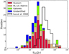 |
Fig. 1. Distribution of the total single dish flux density of the sources, measured at 86 GHz at Pico Veleta or Plateau de Bure during the observations, S86, broken down according to different host galaxy types and compared to the respective distribution for the sources from the sample of Lee et al. (2008). The present survey provides a nearly twofold increase in the number of objects imaged with VLBI at 3 mm. |
2.2. Observations
The survey observations have been made over a total of six days (144 h), scheduled within three separate GMVA sessions. Up to 14 telescopes took part in the observations (see Table 2). The observations were typically scheduled with five scans per hour, each of 300 s in duration. Gaps of five to ten minutes were introduced between the scans for antennae pointing at Effelsberg (Eb) and Pico Veleta (Pv) and for phasing of the Plateau de Bure (Pb) interferometer. This observing scheme yielded the total of 720 scans distributed between 174 observing targets (162 unique radio sources), ensuring that each object was observed with four to five scans distributed over a wide range of hour angles. Despite the rather modest observing time spent on each target, the large number of participating antennae ensured good uv-coverages for all survey sources down to the lowest declinations (see Fig. 2).
Log of survey observations.
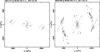 |
Fig. 2. Examples of uv-coverages of the survey observations for a low declination source (left; J1811+1704, δ = +17°) and a high declination source (right; J0642+8811, δ = +88°). |
The observations were performed at a sampling rate of 512 Mbit s−1 and with a two–bit sampling. There were four intermediate frequencies (IFs) in Epoch A and C, and two IFs in Epoch B. The typical baseline sensitivities for a 20 s integration time are ≈0.05 Jy on the Pb–Pv baseline, ≈0.1 Jy on the Eb–Pv baseline, ≈0.2 Jy on the baselines between Eb/Pv and other antennae, and ≈0.4 Jy on the baselines between the VLBA antennae. With such baseline sensitivities and an on-source integration time of about 20 min, the typical point source sensitivity of a survey observation is ∼5 mJy beam−1, which is sufficient to obtain robust images of most of the survey sources.
3. Data processing
3.1. Correlation and fringe fitting
The data were correlated at the DiFX correlator (Deller et al. 2011) of the Max-Planck-Institut für Radioastronomie (MPIfR) at Bonn. After correlation, the data were loaded into AIPS (Astronomical Image Processing System; Greisen et al. 1990). After applying the correlator model, the residual fringe delays and rates were determined and corrected for both within the individual IFs (single-band fringe fitting) and between the IFs (multi-band fringe fitting).
At the first step of the fringe fitting, manual phasecal correction was applied by obtaining the single band delay and delay rate solutions from a scan on a strong source that gives high signal-to-noise ratio (S/N) of the fringe solutions (an S/N ≥ 7 threshold was set) over the typical coherence time (≈20 s) for all the antennae. The resulting fringe solutions were applied to the entire dataset. After the manual phasecal correction, antenna-based global fringe fitting (Schwab & Cotton 1983; Alef & Porcas 1986) was performed, setting the solution interval to the full scan length in order to improve the detection S/N. Pico Veleta was used as the reference antenna for almost all the data. Whenever Pico Veleta was not present in the data, Plateau de Bure or Pie Town were used as the reference antennae. To minimize the chance of false detections, the data were fringe fitted with a S/N threshold of five and a search window width of 200 ns for the fringe delay and 400 mHz for the fringe rate.
Once the global fringe fit was done, the S/N of the fringe solutions were inspected for all the sources, and strong sources which give relatively very high S/N were determined. Whenever feasible, the solutions from those strong sources were interpolated to nearby weak sources, using a procedure similar to that adopted in the similar earlier VLBI survey observations at 86 GHz (cf., Lee et al. 2008). Application of the interpolated solutions has resulted in the detection of amplitude and phase signals for all of the survey targets.
3.2. Amplitude calibration
A priori amplitude calibration was done using the measured values of antenna gain and system temperature. The weather information from each station during the observation was used to correct for the atmospheric opacity. The initial opacity correction was implemented by setting the opacity τ = 0.1 and fitting for the receiver temperatures, Trec. At the second step, the fitted receiver temperatures were used as initial values for fitting simultaneously for τ and Trec.
Participating telescopes.
The accuracy and self-consistency of the amplitude calibration was checked with a procedure developed and used in the earlier 86 GHz survey experiments (Lobanov et al. 2000; Lee et al. 2008). The calibrated visibility data were model fitted for each of the survey targets, using two-dimensional Gaussian components and allowing for scaling the individual antenna gains by a constant factor. The resulting average gain scale corrections are listed in Table 4. The scale offsets are within 25% for most of the antennae, except Metsähovi which had suffered from persistently bad weather during each of the three observing sessions. The averaged offsets are within about 3% of the unity implying that there is no significant bias in the calibration and their rms (root mean square) is less than 10% for each of the three observing epochs. Based on this analysis, we conclude that the a priori amplitude calibration should be accurate to within about 25%, providing a sufficient initial calibration accuracy for the hybrid imaging of the source structure.
Average antenna gain corrections.
List of sources.
3.3. Hybrid imaging and model fitting
After the phase and amplitude calibration was applied on the data, the visibility data were averaged for 10 s for most of the sources and in some cases, the data were averaged for 30 s. The data were then processed in the the Caltech DIFMAP software package (Shepherd et al. 1994), modelling them with circular Gaussian patterns (model fitting; Fomalont 1999) and obtaining hybrid images. The data were not uv-tapered and the imaging was performed using the natural weighting.
The initial model fitting was performed on the calibrated data and was used, in some cases, to facilitate the hybrid imaging. The final model fitting was done on the self-calibrated data resulting from the hybrid imaging. The total number of Gaussian components used for model fitting a given source was determined using the χ2 statistics of the fits. The final models were obtained when the addition of another Gaussian component did not provide a statistically significant change of the χ2 agreement factors (Schinzel et al. 2012).
The hybrid imaging procedure comprised the CLEAN deconvolution (Clark 1980) and self calibration (Cornwell & Fomalont 1999; Cornwell 1995). For most of the objects, the hybrid imaging procedure was initiated with a point source model. For objects with sparse visibility data, the initial Gaussian model fits were used as the initial models. Only visibility phases were allowed to be modified during the initial iterations of the hybrid imaging. At the last step, a single time constant antenna gain correction factor was applied to the visibility amplitudes (hence not allowing for time variable antenna gains in order to avoid the imprint of model errors into data). The parameters of the final images are listed in Table 6, together with the correlated flux densities measured on short and long baselines.
Image parameters.
The quality of the residual noise in the final images, which ideally should have a zero-mean Gaussian distribution, was checked by calculating the expectation value for the maximum absolute flux density |Sr, exp| in a residual image (Lee et al. 2008),
 (1)
(1)
where Npix is the total number of pixels in the image. The quality of the residual noise is given by ξr = Sr/Sr, exp, where Sr is the maximum flux density in the residual image and σr is the rms noise in the residual image. When the residual noise approaches Gaussian noise, ξr tends to 1. If ξr > 1, not all the structure has been adequately recovered; if ξr < 1, the image model has an excessively large number of degrees of freedom (Lobanov et al. 2006). Figure 3 shows the overall distribution of ξr for the residual maps of all the sources in this survey. Column 14 in Table 6 shows the quality factor, ξr obtained for all the 3 mm images implying that the images adequately represent the source structure detected in the visibility data. The Gaussianity of the residual noise is also reflected in the median and the mean of the ξr distributions, which are within 10% of the unity factor.
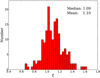 |
Fig. 3. Distribution of the noise quality factor ξr for the residual images of all the sources in the survey. |
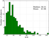 |
Fig. 4. Distribution of the imaging S/N of all the sources in the survey calculated from the ratio of the peak flux density of the map, Sp, to the rms noise in the map, σrms. |
In order to check the effect of the amplitude (antenna gain) corrections applied during the final self calibration step, we compared the visibility amplitudes obtained without and with it. This was done by comparing the ratios of the visibility amplitudes obtained without and with the antenna gain correction on short BS and long BL baselines (see Table 6). The average of the ratios are found to be (1.24 ± 0.18) and (1.01 ± 0.14) for the short and long baselines, respectively. These ratios imply that the amplitude self-calibration did not introduce substantial gain corrections, thus further indicating the overall good quality of the a priori amplitude calibration of the survey data.
3.4. Gaussian models of the source structure
The final self calibrated data were fitted with circular Gaussian components, using the initial model fits as a starting guess. The resulting models were used to obtain the total, Stot, and peak flux density, Speak, the size, d, and the positional offset, (in polar coordinates r,θ) of the component from the brightest region (core) at the base of the jet, taken to be at the coordinate origin. The uncertainties of the model parameters were estimated analytically, based on the S/N of detection of individual components, following Fomalont (1999) and Schinzel et al. (2012):
 (2)
(2)
where σrms is the rms noise in the residual image after substraction of the Gaussian model fit. To assess whether a given component is extended (resolved), the minimum resolvable size of the component was also calculated and compared with the size obtained with the model fitting. The minimum resolvable size, dmin of a Gaussian component is given in Lobanov (2005) as
![Mathematical equation: $$ \begin{aligned} d_\mathrm{min} = \frac{2^{\left(1+\beta /2\right)}}{\pi } \left[ \pi \, a \, b \, \log \left( \frac{S/N+1}{S/N} \right) \right] ^{1/2}, \end{aligned} $$](/articles/aa/full_html/2019/02/aa33122-18/aa33122-18-eq5.gif) (3)
(3)
where a and b are the axes of the restoring beam, S/N is the signal-to-noise ratio, and β is the weighing function that is 0 for natural weighting or 2 for uniform weighting. For components that have size estimates < dmin, the latter is taken as an upper limit of the size and used for estimating the uncertainties of the other model fit parameters of the respective component (see Table 7).
Model fit parameters.
3.5. Brightness temperature estimates
We use the total flux density Stot and size d of the model fit components to estimate the brightness temperature, Tb = Iνc2/2kBν (with ν, kB, and c denoting the observing frequency, the Boltzmann constant, and the light speed, respectively) of the individual emitting regions in the jets.
For a circular Gaussian component, Iν = (4 log2/2)Stot/d2, and the respective brightness temperature can be obtained from
![Mathematical equation: $$ \begin{aligned} T_\mathrm{b} \mathrm{[K]} = 1.22 \times 10^{12} \left(\frac{S_\mathrm{tot} }{\mathrm{Jy} }\right) \left(\frac{d}{\mathrm{mas} }\right)^{-2} \left(\frac{\nu }{\mathrm{GHz} }\right)^{-2} (1+z). \end{aligned} $$](/articles/aa/full_html/2019/02/aa33122-18/aa33122-18-eq6.gif) (4)
(4)
The factor (1 + z) reflects the effect of the cosmological redshift z on the observed brightness temperature. For the sources with unknown redshift, we calculated the brightness temperature simply in the observer’s frame of reference. If the size of the Gaussian component d is less than dmin, given by Eq. (3), the latter is used for estimating the lower limit on Tb.
In addition to this estimate, we also use visibility-based estimates of brightness temperature (Lobanov 2015) and calculate the minimum brightness temperature,
![Mathematical equation: $$ \begin{aligned} T_\mathrm{b,min} \mathrm{[K]} = 3.09 \left(\frac{V_{\mathrm{q} }}{\mathrm{mJy} }\right) \left(\frac{B_{\mathrm{L} }}{\mathrm{km} }\right)^{2}, \end{aligned} $$](/articles/aa/full_html/2019/02/aa33122-18/aa33122-18-eq7.gif) (5)
(5)
and limiting resolved brightness temperature,
![Mathematical equation: $$ \begin{aligned} T_\mathrm{b,lim} \mathrm{[K]} = 1.14 \left(\frac{V_{\mathrm{q} }+\sigma _\mathrm{q} }{\mathrm{mJy} }\right)\left(\frac{B_{\mathrm{L} }}{\mathrm{km} }\right)^{2} \left(\ln \frac{V_\mathrm{q} +\sigma _\mathrm{q} }{V_\mathrm{q} }\right)^{-1}, \end{aligned} $$](/articles/aa/full_html/2019/02/aa33122-18/aa33122-18-eq8.gif) (6)
(6)
directly from the visibility amplitude, Vq, and its error, σq, measured at a given long baseline, BL, in the survey data.
4. Results
4.1. Images
Using the procedures described above, we have made hybrid maps of all 174 observations of 162 unique sources in this survey. For 138 objects, the survey provides the first ever VLBI images made at 86 GHz. Most of the imaged sources show extended radio emission, revealing the jet morphology down to sub-parsec scales. For a small number of weaker sources with poor uv-coverages, only the brightest core at the base of the jet could be imaged. To illustrate our results, we present images of four weak target radio sources J1130+3815, J0700+1709, J1044+8054 and J0748+2400 in Fig. 6 (a total of 174 contour maps of 162 unique sources imaged at 3 mm in this survey are available in Appendix A).
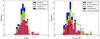 |
Fig. 5. Distribution of the correlated flux densities corresponding to the longest baselines, SL (left) and the total clean image flux density, SCLEAN of the survey targets broken down according to different host galaxy types (right). The distribution of SCLEAN for the sources in this survey is also compared with the respective distribution for the sources from the sample of Lee et al. (2008) on the right panel. |
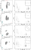 |
Fig. 6. GMVA maps of J1130+3815, J0700+1709, J1044+8054, and J0748+2400 (left panel), shown together with the respective radial amplitude distributions (right panel) and uv-coverages (inset in the right panel) of the respective visibility datasets. The contouring of images is made at |
Figure 5 illustrates the properties of the survey sample by plotting the distributions of the correlated flux density, SL, measured on long baselines and the total flux density, SCLEAN, in the CLEAN images of the observed sources. Both distributions indicate that objects with flux densities ≳80 mJy can be successfully detected and imaged with the survey data, signifying the sensitivity improvement by a factor of approximately two compared to the observations presented in Lee et al. (2008). The mean of the correlated flux density at the longest baseline, SL, is 0.2 Jy. Amongst 157 sources whose SL can be measured at projected baselines longer than 2000 Mλ, 135 sources have an SL greater than 0.1 Jy.
In Table 6, we present the basic parameters of the images, listing (1) source name, (2) observing epoch, (3) single dish 86 GHz flux density, S86, measured at Pico Veleta or Plateau de Bure, (4) correlated flux density on the shortest baseline, SS, (5) shortest baseline, BS, (6) correlated flux density on the longest baseline, SL, (7) longest baseline, BL, (8) major axis, Ba, (9) minor axis, Bb, and (10) position angle, BPA of the major axis of the restoring beam, (11) total CLEAN flux density, Stot, and (12) peak flux density, Speak, in the image, (13) image rms noise, σrms, and (14) the quality factor of the residual noise in the image, ξr.
Table 7 summarizes the model fits obtained for all of the survey sources providing (1) the source name, (2) observing epoch, (3) sequential number of the Gaussian component, (4) total flux density, St, and (5) peak flux density, Speak, of the component, (6) size, d, of the component, (7) separation, r, and (8) position angle, θ of the component with respect to the brightest feature in the model (core, taken to be located at the coordinate origin), (9) brightness temperature, Tb, mod, estimated from the model fit, and (10) minimum, Tb, min and (11) limiting resolved, Tb, lim, brightness temperatures estimated from the visibility amplitudes (Lobanov 2015) at the longest baselines given in Col. 7 in Table 6.
Table 7 contains the model fit parameters for a total 174 VLBI cores and 205 jet components, with 42 and 37 of these unresolved, as reflected also in the lower limits of the model-fit-based brightness temperature estimates, Tb, mod, listed for these components.
4.2. Source compactness
Compactness of the source structure can be evaluated by comparing the single dish flux density, S86, listed in Table 6, to the total clean flux density, SCLEAN, listed in Table 6 and the core flux density, SCORE, listed in Table 7, to the total clean flux density, SCLEAN. These comparisons are presented in Fig. 7.
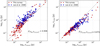 |
Fig. 7. Compactness parameters, S86/SCLEAN and Score/SCLEAN are shown on the left and right panel respectively, where S86 is the single dish 86 GHz flux density measured at Pico Veleta or Plateau de Bure. The Pearson correlation coefficients = 0.908 and = 0.874 are obtained for the combined data from this survey and Lee et al. (2008). |
To study the relation between the total and VLBI flux densities, we apply the Pearson correlation test. The Pearson correlation coefficient calculated for S86 and SCLEAN gives a significant value of 0.924 for this survey and 0.908 for this survey combined with the results from Lee et al. (2008). The respective plot in the left panel of Fig. 7 indicates that almost all the flux measured by a single dish (here Pv or PdB) is recovered in the VLBI clean flux. The median of the core dominance index defined as SCORE/SCLEAN is 0.84, and the two are also correlated, as demonstrated in the right panel of Fig. 7.
Figure 7 shows that the stronger sources have more structures (right panel) some of which are completely resolved out even on the shortest baselines of the survey observations (left panel). A small number of cases for which SCLEAN > S86 or SCORE > SCLEAN are observed for the weaker objects. These can be reconciled with the errors in the measurements, and they essentially imply very compact objects, with S86 ≃ SCLEAN and SCORE ≃ SCLEAN, respectively.
4.3. Brightness temperatures
In our further analysis, we use the model-fit-based and visibility-based estimates of the brightness temperature of the VLBI bright core (base) and the inner (rproj < 1 pc) jet components, taking into account the resolution limits of the data at 3 mm. The brightness temperature estimates for the jet cores in our sample range from 2.5 × 10⁹ K to 1.3 × 10¹² K. The brightness temperature estimates for the inner jet components in our sample range from 7.0 × 10⁷ K to 4.0 × 10¹¹ K. The median and mean of the brightness temperature distribution for the core regions are 8.6 × 10¹⁰ K and 1.8 × 10¹¹ K, respectively. For the inner jet components, the respective figures are 7.2 × 10⁹ K and 2.2 × 10¹⁰ K. This shows that the brightness temperature drops by approximately an order of magnitude already on sub-parsec scales in the jets, with inverse Compton, synchrotron, and adiabatic losses subsequently dominating the energy losses (cf. Marscher 1995; Lobanov & Zensus 1999). Only 8% of the jet cores show a brightness temperature greater than 5 × 10¹¹ K and only 3% have a brightness temperature greater than 1012 K.
We also inspect the distribution of the minimum and maximum limiting brightness temperature of the core components (using averaged values of brightness temperature for objects with multiple observations) in the sample, making these estimates from the visibility amplitudes on the longest baselines (Lobanov 2015). The minimum, Tb, min, and limiting, Tb, lim, brightness temperatures are given in Table 7, in Cols. 10 and 11, respectively.
The median and mean of the maximum limiting brightness temperature distribution for the core regions is 1.06 × 10¹¹ K and 3.0 × 10¹¹ K, respectively. We find that the limiting Tb, lim correlates well with Tb, mod estimated from imaging method as seen in Fig. 8, supporting the fidelity of Tb, mod measurements obtained from model fitting. The residual logarithmic distribution of the Tb, mod/Tb, lim ratio is well approximated by the Gaussian PDF, with mean value, μ = 0.001 and standard deviation, σ = 0.46.
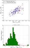 |
Fig. 8. Comparison of Tb, mod measured from circular Gaussian representation of source structure and Tb, lim estimated from the interferometric visibilities at uv-radii within 10% of the maximum baseline Bmax in the data for a given source (top panel). Correlation between the two distributions is illustrated by the residual logarithmic distribution of the Tb, mod/Tb, limit ratio (bottom panel), which is well approximated by the Gaussian distribution with μ = 0.001 and σ = 0.46. |
5. Discussion
5.1. Modelling the observed brightness temperatures
The brightness temperature distribution can be used for obtaining estimates of the conditions in the extra galactic radio sources and to test the models proposed for the inner jets (Marscher 1995; Lobanov et al. 2000; Homan et al. 2006; Lee et al. 2008). A basic population model (Lobanov et al. 2000) can be used for representing the observed brightness temperature distribution under the assumption that the jets have the same intrinsic brightness temperature, T0, Lorentz factor, Γj, and synchrotron spectral index, α (Sν ∝ να), and they are randomly oriented in space (within the limits of viewing angles, θ, required by Doppler boosting bias). The jets are also assumed to remain straight within the spatial scales (∼0.5−10 pc) probed by the observations.
The assumptions of single values of T0 and Γj describing the whole sample are clearly simplified, as jets are known to feature a range of Lorentz factors (see Lister et al. 2016, and references therein). However, as has been shown earlier (Lobanov et al. 2000), factoring a distribution of Lorentz factors into the present model is not viable without amending the brightness temperature measurements with additional information, preferably about the apparent speeds of the target sources. We are currently compiling such a combined database, and will engage in a more detailed modelling of the compact jets after the completion of this database.
In a population of jets described by the settings summarized above, the measured brightness temperature, Tb, is determined solely by the relativistic Doppler boosting of the jet emission. Therefore, the observed brightness temperature, Tb, can be related to the intrinsic brightness temperature, T0, so that Tb = T0 δ1/ϵ, where the power index ϵ is 1/(2 − α) for a continuous jet (steady state jet) and 1/(3 − α) for a jet with spherical blobs (or optically thin “plasmoids”), and δ is the Doppler factor.
The probability of finding a radio source with the brightness temperature Tb in such a population of sources is
![Mathematical equation: $$ \begin{aligned} p(T_\mathrm{b} ) \propto \Bigg [ \frac{2\,\Gamma _{j}\left(T_\mathrm{b} /{T_\mathrm{0} }\right)^\epsilon - \left(T_\mathrm{b} /{T_\mathrm{0} }\right)^{2\epsilon } - 1}{\Gamma _\mathrm{j} ^{2} - 1}\Bigg ]^{\frac{1}{2}}. \end{aligned} $$](/articles/aa/full_html/2019/02/aa33122-18/aa33122-18-eq10.gif) (7)
(7)
The lower end of the observed distribution of brightness temperatures depends on the sensitivity of VLBI data since the flux of the observed sample is biased by Doppler boosting (Lobanov et al. 2000). The lowest brightness temperature that can be measured from our data, Tb, sens, can be obtained from
![Mathematical equation: $$ \begin{aligned} T_{\mathrm{b,sens} }{\mathrm{[K]} } = 1.65 \times 10^{5} \left(\frac{\sigma _{\rm rms}}{\mathrm{mJy\,beam^{-1}}}\right) \left(\frac{b}{\mathrm{mas}}\right)^{-2}, \end{aligned} $$](/articles/aa/full_html/2019/02/aa33122-18/aa33122-18-eq11.gif) (8)
(8)
where σrms is the array sensitivity in mJy beam−1 and b is the average size of the resolving beam. In this survey, the typical observation time on a target source Δt is 20 min and bandwidth is 128 MHz. Therefore, the value of beam size for the sources in this survey is 0.12 mas and the σrms of the array is 0.54 mJy beam−1. Thus, we have obtained a 3σ level estimation of Tb, sens as 2.0 × 10⁸ K using Eq. (8), which is set as the lowest brightness temperature in modelling.
We normalize the results obtained from Eq. (7) to the number of objects in the lowest bin of the histogram. For our modelling, we first make a generic assumption of α = −0.7 (homogeneous synchrotron source) and use Γj ≈ 10 implied from the kinematic analysis of the MOJAVE VLBI survey data (Lister et al. 2016). We assume that the jet is continuous, so ϵ = 0.37 is taken. For the population modelling analysis, we have included the data from Lobanov et al. (2000), Lee et al. (2008), and the present survey, yielding a final database of 271 VLBI core components and 344 jet components. For objects with multiple measurements, we have used the median of the measurements. The resulting model distributions obtained for various values of T0 are shown in Figs. 9–10 for the VLBI cores and the inner jet components, respectively.
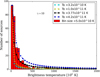 |
Fig. 9. Distribution of the brightness temperatures, Tb, measured in the core components and represented by the population models calculated for Γj = 10 and different values of T0. The best approximation of the observed Tb distribution is obtained with To, core = |
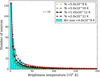 |
Fig. 10. Distribution of the brightness temperatures, Tb, measured in the inner jet components and represented by the population models calculated for Γj = 10 and different values of T0. The best approximation of the observed Tb distribution is obtained with |
This approach yields T0, core =  for the VLBI cores and
  for the inner jet components. The estimated T0, core is in good agreement with the inverse Compton limit of ≃5.0 × 10¹¹ K (Kellermann & Pauliny-Toth 1969), beyond which the inverse Compton effect causes rapid electron energy losses and extinguishes the synchrotron radiation. The inferred T0, jet of jet components are about a factor of three higher than the equipartition limit of ≃5 × 10¹⁰ K (Readhead et al. 1983) for which the magnetic field energy and particle energy are in equilibrium. This may indicate that opacity is still non-negligible in these regions of the flow. The intrinsic brightness temperature obtained for the cores is within the upper limit 5.0 × 10¹¹ K predicted for the population modelling of the cores (Lobanov et al. 2000).
A simultaneous fit for T0 and Γj is impeded by the implicit correlation,  (with a ≈ 2–3), between these two parameters, as implied by Eq. (7). This is also illustrated in Fig. 11, from which a dependence
 ![Mathematical equation: $ {T_{\rm{0}}}[{\rm{K}}] \approx (7.7 \times {10^8}){\mkern 1mu} \Gamma _{\rm{j}}^{2.7} $](/articles/aa/full_html/2019/02/aa33122-18/aa33122-18-eq17.gif) can be inferred for the fit to the brightness temperatures measured in the VLBI cores. This correlation between T0 and Γj precludes simultaneously fitting for both these parameters, and hence the Lorentz factor has to be constrained (or assumed) separately. One should also keep in mind that this correlation results from the model description and does not have an immediate physical implication. Equation (7) clearly shows that the predicted distribution of Tb is valid within the range
can be inferred for the fit to the brightness temperatures measured in the VLBI cores. This correlation between T0 and Γj precludes simultaneously fitting for both these parameters, and hence the Lorentz factor has to be constrained (or assumed) separately. One should also keep in mind that this correlation results from the model description and does not have an immediate physical implication. Equation (7) clearly shows that the predicted distribution of Tb is valid within the range
 (9)
(9)
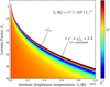 |
Fig. 11. Two-dimensional χ2 distribution plot in the Γj – T0 space, calculated for the brightness temperatures measured in the VLBI cores. The blank area shows the ranges of the parameter space disallowed by the observed distribution. The distribution of the χ2 values indicates a (Γj–T0) correlation, with |
![Mathematical equation: $ {T_{\rm{0}}}[{\rm{K}}] \approx (7.7 \times {10^8}){\mkern 1mu} \Gamma _{\rm{j}}^{2.7} $](/articles/aa/full_html/2019/02/aa33122-18/aa33122-18-eq19.gif)
The region outside this range is represented by the blank area in Fig. 11.
The intrinsic brightness temperature we obtained is higher than the mean and median observed brightness temperature Tb. This is readily explained by the Doppler deboosting. For a given viewing angle, θ, sources with Γj > 1/θ would be deboosted so that the observed brightness temperature will be reduced below its intrinsic value. It can be easily shown that the observed and intrinsic brightness temperatures are equal if the jet viewing angle is given by
![Mathematical equation: $$ \begin{aligned} \theta _\mathrm{eq} = \mathrm{arc\,cos} \left[ \frac{1- (1/\Gamma _\mathrm{j} )\,\,(T_\mathrm{0} /T_\mathrm{b} )^{\epsilon }}{\sqrt{1-\Gamma _\mathrm{j} ^{-2}}} \right]\cdot \end{aligned} $$](/articles/aa/full_html/2019/02/aa33122-18/aa33122-18-eq20.gif) (10)
(10)
For the VLBI cores, the mean of the observed Tb is 1.8 × 10¹¹ K and intrinsic T0, core is 3.77 × 10¹¹ K, therefore, the resulting θeq = 29° for Γj = 10 and ϵ = 0.37. In this case any object observed at a larger viewing angle would be deboosted resulting in a lower observed Tb than intrinsic T0.
5.2. Testing the adiabatic expansion of jets
As discussed in Sects. 4.3 and 5.1, intrinsic T0 and the observed Tb in core and jets show that the brightness temperature drops by approximately a factor of two to ten already on sub-parsec scales in the jets. This evolution might occur with the inverse Compton, synchrotron, and adiabatic losses subsequently dominating the energy losses (cf., Marscher 1995; Lobanov & Zensus 1999).
For four objects in our data (3C84, 0716+714, 3C454.3, and J2322+507) for which multiple jet components have been identified during the model fitting, it is possible to use the brightness temperatures of the jet components to test whether the evolution of the jet brightness on sub parsec scales could be explained by adiabatic energy losses (Marscher & Gear 1985). For this analysis, we assume that the jet components are independent relativistic shocks embedded in the jet plasma, which has a power-law distribution N(E) dE ∝ E−sdE, where s is the energy spectral index that depends on spectral index α as α = (1 − s)/2, and is pervaded by the magnetic field B ∝ d−a, where d is the width of the jet and a depends on the type of magnetic field (a = 1 for poloidal magnetic field and 2 for toroidal magnetic field). With these assumptions, we can relate the brightness temperatures, Tb, J, of the jet components to the brightness temperature, Tb, C, of the core (Lobanov et al. 2000; Lee et al. 2008),
 (11)
(11)
where dJ and dC are the measured sizes of the jet component and core, respectively, and
 (12)
(12)
Assuming the synchrotron emission with spectral index α = −0.5, we use s = 2.0 and adopt a = 1.0 for the description of the magnetic field in the jet. With these assumptions, we calculate the predicted Tb, J for individual jet components and compare them in Fig. 12 to the measured brightness temperatures. The measured and predicted values of brightness temperature agree well, and this suggests that the jet components can be viewed as adiabatically expanding relativistic shocks (cf., Kadler et al. 2004; Pushkarev & Kovalev 2012; Kravchenko et al. 2016).
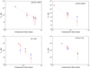 |
Fig. 12. Changes of the brightness temperature as a funcion of jet width for four sources – J2322+5037, J1033+6051, 3C 345, and 0716+714 from this survey. Blue squares denote the measured Tb from this survey. The red circles connected with a dotted line represent theoretically expected Tb under the assumption of adiabatic jet expansion. The initial brightness temperature in each jet is assumed to be the same as that measured in the VLBI core. |
6. Summary
We have used the Global Millimeter VLBI Array (GMVA) to conduct a large global 86 GHz VLBI survey comprising 174 snapshot observations of 162 unique targets selected from a sample of compact radio sources. The survey observations have reached a typical baseline sensitivity of 0.1 Jy and a typical image sensitivity of 5 mJy beam−1, owing to the increased recording bandwidth of the GMVA observations and the participation of very sensitive European antennae at Pico Veleta and Plateau de Bure. All of the 162 objects have been detected and imaged, thereby increasing the total number of AGN imaged with VLBI at 86 GHz by a factor of ∼1.5. We imaged 138 sources for the first time with VLBI at 86 GHz through this survey.
We have used Gaussian model fitting to represent the structure of the observed sources and estimate the flux densities and sizes of the core and jet components. We used the model fit parameters and visibility data on the longest baselines to make independent estimates of brightness temperatures at the jet base as described by the most compact and bright “VLBI core” component. These estimates are consistent with each other. For sources with extended structure detected, the model fit parameters have been also used to calculate brightness temperature in the jet components downstream from the core. The apparent brightness temperature estimates for the jet cores in our sample range from 2.5 × 10⁹ K to 1.3 × 10¹² K, with the mean value of 1.8 × 10¹¹ K. The brightness temperature estimates for the inner jet components in our sample range from 7.0 × 10⁷ K to 4.0 × 10¹¹ K. The overall amplitude calibration error for the observations is about 25%.
We describe the observed brightness temperature distributions by a basic population model which assumes that all jets are intrinsically similar and can be described by a single value of the intrinsic brightness temperature, T0, and Lorentz factor, Γj. The population modelling shows that our data are consistent with a population of sources that has  in the VLBI cores and
  in the jets, both obtained for Γj = 10 adopted from the kinematic analysis of the MOJAVE VLBI survey of AGN jets (Lister et al. 2016). A correlation between T0 and Γj inherent to the model description precludes fitting for these two parameters simultaneously. We find that a relation T0[K] ≈ (7.7 × 10⁸) Γj2.7 is implied for this modelling framework by the survey data. For sources with sufficient structural detail, there is an agreement between the brightness temperatures measured in multiple components along the jet and the predicted brightness temperatures for relativistic shocks with adiabatic losses dominating the emission.
The results of the survey can be combined with brightness temperature measurements made from VLBI observations at lower frequencies (e.g., Kovalev et al. 2005; Petrov et al. 2007) to study the evolution of T0 with frequency and along the jet (Lee et al. 2008, 2016). This approach can be used to better constrain the bulk Lorentz factor and the intrinsic brightness temperature, to distinguish between the acceleration and deceleration scenario for the flow (cf., Marscher 1995), and to test several alternative acceleration scenarios including hydrodynamic acceleration (Bodo et al. 1985), acceleration by tangled magnetic field (Heinz & Begelman 2000), and magnetohydrodynamics acceleration (Vlahakis & Königl 2004).
The complete set of images of all the target sources are presented in Appendix A.
Very Long Baseline Array of the National Radioastronomy Observatory, Socorro, NM; https://www.lbo.us/
Acknowledgments
We thank the staff of the observatories participating in the GMVA, the MPIfR Effelsberg 100 m telescope, the IRAM Plateau de Bure Interferometer, the IRAM Pico Veleta 30 m telescope, the Metsähovi Radio Observatory, the Onsala Space Observatory, and the VLBA. The VLBA is an instrument of the National Radio Astronomy Observatory, which is a facility of the National Science Foundation operated under cooperative agreement by Associated Universities, Inc. This research has made use of the NASA/IPAC Extragalactic Database (NED) which is operated by the Jet Propulsion Laboratory, California Institute of Technology, under contract with the National Aeronautics and Space Administration. This research has made use of the SIMBAD database, operated at CDS, Strasbourg, France and also the Sloan Digital Sky Survey (SDSS). This research has made use of data obtained with the Global Millimeter VLBI Array (GMVA), which consists of telescopes operated by the MPIfR, IRAM, Onsala, Metsahovi, Yebes, and the VLBA. The VLBA is an instrument of the National Radio Astronomy Observatory. The National Radio Observatory is a facility of the National Science Foundation operated under the cooperative agreement by Associated Universities. The data were correlated at the MPIfR in Bonn, Germany. Dhanya G. Nair is a member of the International Max Planck Research School (IMPRS) for Astronomy and Astrophysics at the Universities of Bonn and Cologne. Thanks to Biagina Boccardi, Jun Liu, Laura Vega García, Jae-Young Kim, Ioannis Myserlis, Vassilis Karamanavis, Jeff Hodgson, Shoko Koyama, Bindu Rani and Karl M. Menten for their valuable suggestions and support in this research. The author also thanks Walter Alef and Alessandra Bertarini for helping in the correlation of the 86 GHz VLBI data used in this research. Thanks to Uwe Bach and Salvador Sánchez who have helped in the observation and calibration at Effelsberg radio telescope and IRAM Pico Veleta radio telescope, respectively. Sang-Sung Lee was supported by the National Research Foundation of Korea (NRF) grant funded by the Korea government (MSIP) (No. NRF-2016R1C1B2006697). Yuri Y. Kovalev was supported in part by the government of the Russian Federation (agreement 05.Y09.21.0018) and by the Alexander von Humboldt Foundation.
References
- Alef, W., & Porcas, R. W. 1986, A&A, 168, 365 [NASA ADS] [Google Scholar]
- Asada, K., Nakamura, M., Doi, A., Nagai, H., & Inoue, M. 2014, ApJ, 781, L2 [NASA ADS] [CrossRef] [Google Scholar]
- Beasley, A. J., Dhawan, V., Doeleman, S., & Phillips, R. B. 1997, in Millimeter-VLBI Science Workshop, eds. R. Barvainis, & R. B. Phillips, 53 [Google Scholar]
- Boccardi, B., Krichbaum, T. P., Bach, U., Bremer, M., & Zensus, J. A. 2016, A&A, 588, L9 [NASA ADS] [CrossRef] [EDP Sciences] [Google Scholar]
- Bodo, G., Ferrari, A., Massaglia, S., & Tsinganos, K. 1985, A&A, 149, 246 [NASA ADS] [Google Scholar]
- Clark, B. G. 1980, A&A, 89, 377 [NASA ADS] [Google Scholar]
- Cohen, M. H., Lister, M. L., Homan, D. C., et al. 2007, ApJ, 658, 232 [NASA ADS] [CrossRef] [Google Scholar]
- Cornwell, T. 1995, in Very Long Baseline Interferometry and the VLBA, eds. J. A. Zensus, P. J. Diamond, & P. J. Napier, ASP Conf. Ser., 82, 39 [NASA ADS] [Google Scholar]
- Cornwell, T., & Fomalont, E. B. 1999, in Synthesis Imaging in Radio Astronomy II, eds. G. B. Taylor, C. L. Carilli, & R. A. Perley, ASP Conf. Ser., 180, 187 [NASA ADS] [Google Scholar]
- Deller, A. T., Brisken, W. F., Phillips, C. J., et al. 2011, PASP, 123, 275 [NASA ADS] [CrossRef] [Google Scholar]
- Fomalont, E. B. 1999, in Synthesis Imaging in Radio Astronomy II, eds. G. B. Taylor, C. L. Carilli, & R. A. Perley, ASP Conf. Ser., 180, 301 [NASA ADS] [Google Scholar]
- Greisen, E. W. 1990, in Acquisition, Processing and Archiving of Astronomical Images, eds. G. Longo, & G. Sedmak, 125 [Google Scholar]
- Heinz, S., & Begelman, M. C. 2000, ApJ, 535, 104 [NASA ADS] [CrossRef] [Google Scholar]
- Homan, D. C., Kovalev, Y. Y., Lister, M. L., et al. 2006, ApJ, 642, L115 [NASA ADS] [CrossRef] [Google Scholar]
- Kadler, M., Ros, E., Lobanov, A. P., Falcke, H., & Zensus, J. A. 2004, A&A, 426, 481 [NASA ADS] [CrossRef] [EDP Sciences] [Google Scholar]
- Kellermann, K. I., & Pauliny-Toth, I. I. K. 1969, ApJ, 155, L71 [NASA ADS] [CrossRef] [Google Scholar]
- Kellermann, K. I., Lister, M. L., Homan, D. C., et al. 2004, ApJ, 609, 539 [NASA ADS] [CrossRef] [Google Scholar]
- Kovalev, Y. Y., Kellermann, K. I., Lister, M. L., et al. 2005, AJ, 130, 2473 [NASA ADS] [CrossRef] [Google Scholar]
- Kravchenko, E. V., Kovalev, Y. Y., Hovatta, T., & Ramakrishnan, V. 2016, MNRAS, 462, 2747 [NASA ADS] [CrossRef] [Google Scholar]
- Lee, S.-S., Lobanov, A. P., Krichbaum, T. P., et al. 2008, AJ, 136, 159 [NASA ADS] [CrossRef] [Google Scholar]
- Lee, S.-S., Lobanov, A. P., Krichbaum, T. P., & Zensus, J. A. 2016, ApJ, 826, 135 [Google Scholar]
- Lister, M. L. 2003, ApJ, 599, 105 [NASA ADS] [CrossRef] [Google Scholar]
- Lister, M. L., & Homan, D. C. 2005, AJ, 130, 1389 [NASA ADS] [CrossRef] [Google Scholar]
- Lister, M. L., Cohen, M. H., Homan, D. C., et al. 2009, AJ, 138, 1874 [NASA ADS] [CrossRef] [Google Scholar]
- Lister, M. L., Aller, M. F., Aller, H. D., et al. 2016, AJ, 152, 12 [NASA ADS] [CrossRef] [Google Scholar]
- Lobanov, A. P. 2005, ArXiv e-prints [arXiv:astro-ph/0503225] [Google Scholar]
- Lobanov, A. P. 2015, A&A, 574, A84 [NASA ADS] [CrossRef] [EDP Sciences] [Google Scholar]
- Lobanov, A. P., & Zensus, J. A. 1999, ApJ, 521, 509 [NASA ADS] [CrossRef] [Google Scholar]
- Lobanov, A. P., Krichbaum, T. P., Graham, D. A., et al. 2000, A&A, 364, 391 [NASA ADS] [Google Scholar]
- Lobanov, A. P., Krichbaum, T. P., Witzel, A., & Zensus, J. A. 2006, PASJ, 58, 253 [NASA ADS] [CrossRef] [Google Scholar]
- Lonsdale, C. J., Doeleman, S. S., & Phillips, R. B. 1998, AJ, 116, 8 [NASA ADS] [CrossRef] [Google Scholar]
- Marscher, A. P. 1995, Proc. Nat. Acad. Sci., 92, 11439 [NASA ADS] [CrossRef] [Google Scholar]
- Marscher, A. P., & Gear, W. K. 1985, ApJ, 298, 114 [NASA ADS] [CrossRef] [Google Scholar]
- Mertens, F., Lobanov, A. P., Walker, R. C., & Hardee, P. E. 2016, A&A, 595, A54 [NASA ADS] [CrossRef] [EDP Sciences] [Google Scholar]
- Petrov, L., Hirota, T., Honma, M., et al. 2007, AJ, 133, 2487 [NASA ADS] [CrossRef] [Google Scholar]
- Pushkarev, A. B., & Kovalev, Y. Y. 2012, A&A, 544, A34 [NASA ADS] [CrossRef] [EDP Sciences] [Google Scholar]
- Rantakyrö, F. T., Baath, L. B., Backer, D. C., et al. 1998, A&AS, 131, 451 [NASA ADS] [CrossRef] [EDP Sciences] [Google Scholar]
- Readhead, A. C. S., Mason, C. R., Mofett, A. T., et al. 1983, Nature, 303, 504 [NASA ADS] [CrossRef] [Google Scholar]
- Rogers, A. E. E., Phillips, R. B., & Lonsdale, C. J. 1995, BAAS, 27, 1300 [NASA ADS] [Google Scholar]
- Schinzel, F. K., Lobanov, A. P., Taylor, G. B., et al. 2012, A&A, 537, A70 [NASA ADS] [CrossRef] [EDP Sciences] [Google Scholar]
- Schwab, F. R., & Cotton, W. D. 1983, AJ, 88, 688 [NASA ADS] [CrossRef] [Google Scholar]
- Shepherd, M. C., Pearson, T. J., & Taylor, G. B. 1994, BAAS, 26, 987 [NASA ADS] [Google Scholar]
- Vermeulen, R. C., & Cohen, M. H. 1994, ApJ, 430, 467 [NASA ADS] [CrossRef] [Google Scholar]
- Vlahakis, N., & Königl, A. 2004, ApJ, 605, 656 [NASA ADS] [CrossRef] [Google Scholar]
- Wenger, M., Ochsenbein, F., Egret, D., et al. 2000, A&AS, 143, 9 [NASA ADS] [CrossRef] [EDP Sciences] [Google Scholar]
Appendix A: Images, visibility amplitude distributions, and uv-coverages of the survey targets
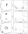 |
Fig. A.1. A total of 174 contour maps of 162 unique sources imaged at 3 mm in this survey (left panel), shown together with the respective radial amplitude distributions (right panel) and uv-coverages (inset in the right panel) of the respective visibility datasets. The contouring of images is made at |

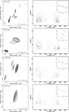 |
Fig. A.1. continued. |
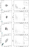 |
Fig. A.1. continued. |
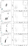 |
Fig. A.1. continued. |
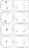 |
Fig. A.1. continued. |
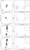 |
Fig. A.1. continued. |
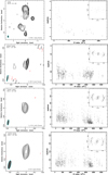 |
Fig. A.1. continued. |
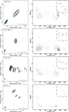 |
Fig. A.1. continued. |
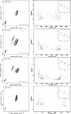 |
Fig. A.1. continued. |
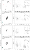 |
Fig. A.1. continued. |
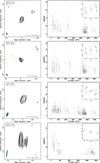 |
Fig. A.1. continued. |
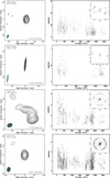 |
Fig. A.1. continued. |
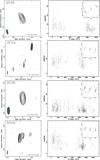 |
Fig. A.1. continued. |
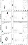 |
Fig. A.1. continued. |
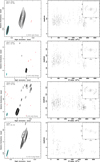 |
Fig. A.1. continued. |
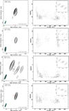 |
Fig. A.1. continued. |
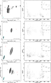 |
Fig. A.1. continued. |
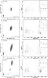 |
Fig. A.1. continued. |
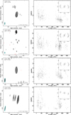 |
Fig. A.1. continued. |
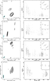 |
Fig. A.1. continued. |
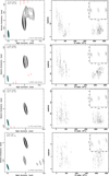 |
Fig. A.1. continued. |
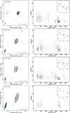 |
Fig. A.1. continued. |
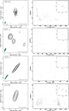 |
Fig. A.1. continued. |
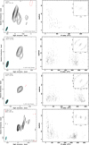 |
Fig. A.1. continued. |
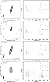 |
Fig. A.1. continued. |
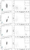 |
Fig. A.1. continued. |
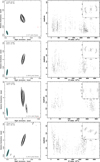 |
Fig. A.1. continued. |
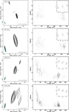 |
Fig. A.1. continued. |
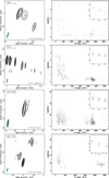 |
Fig. A.1. continued. |
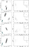 |
Fig. A.1. continued. |
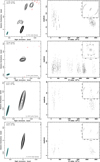 |
Fig. A.1. continued. |
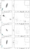 |
Fig. A.1. continued. |
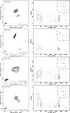 |
Fig. A.1. continued. |
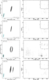 |
Fig. A.1. continued. |
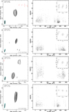 |
Fig. A.1. continued. |
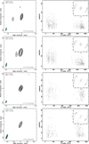 |
Fig. A.1. continued. |
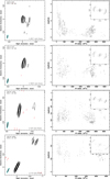 |
Fig. A.1. continued. |
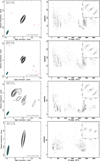 |
Fig. A.1. continued. |
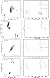 |
Fig. A.1. continued. |
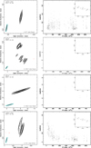 |
Fig. A.1. continued. |
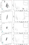 |
Fig. A.1. continued. |
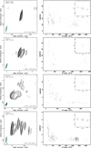 |
Fig. A.1. continued. |
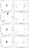 |
Fig. A.1. continued. |
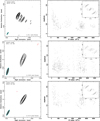 |
Fig. A.1. continued. |
All Tables
All Figures
|
Fig. 1. Distribution of the total single dish flux density of the sources, measured at 86 GHz at Pico Veleta or Plateau de Bure during the observations, S86, broken down according to different host galaxy types and compared to the respective distribution for the sources from the sample of Lee et al. (2008). The present survey provides a nearly twofold increase in the number of objects imaged with VLBI at 3 mm. |
| In the text | |
|
Fig. 2. Examples of uv-coverages of the survey observations for a low declination source (left; J1811+1704, δ = +17°) and a high declination source (right; J0642+8811, δ = +88°). |
| In the text | |
|
Fig. 3. Distribution of the noise quality factor ξr for the residual images of all the sources in the survey. |
| In the text | |
|
Fig. 4. Distribution of the imaging S/N of all the sources in the survey calculated from the ratio of the peak flux density of the map, Sp, to the rms noise in the map, σrms. |
| In the text | |
|
Fig. 5. Distribution of the correlated flux densities corresponding to the longest baselines, SL (left) and the total clean image flux density, SCLEAN of the survey targets broken down according to different host galaxy types (right). The distribution of SCLEAN for the sources in this survey is also compared with the respective distribution for the sources from the sample of Lee et al. (2008) on the right panel. |
| In the text | |
|
Fig. 6. GMVA maps of J1130+3815, J0700+1709, J1044+8054, and J0748+2400 (left panel), shown together with the respective radial amplitude distributions (right panel) and uv-coverages (inset in the right panel) of the respective visibility datasets. The contouring of images is made at |
| In the text | |
|
Fig. 7. Compactness parameters, S86/SCLEAN and Score/SCLEAN are shown on the left and right panel respectively, where S86 is the single dish 86 GHz flux density measured at Pico Veleta or Plateau de Bure. The Pearson correlation coefficients = 0.908 and = 0.874 are obtained for the combined data from this survey and Lee et al. (2008). |
| In the text | |
|
Fig. 8. Comparison of Tb, mod measured from circular Gaussian representation of source structure and Tb, lim estimated from the interferometric visibilities at uv-radii within 10% of the maximum baseline Bmax in the data for a given source (top panel). Correlation between the two distributions is illustrated by the residual logarithmic distribution of the Tb, mod/Tb, limit ratio (bottom panel), which is well approximated by the Gaussian distribution with μ = 0.001 and σ = 0.46. |
| In the text | |
|
Fig. 9. Distribution of the brightness temperatures, Tb, measured in the core components and represented by the population models calculated for Γj = 10 and different values of T0. The best approximation of the observed Tb distribution is obtained with To, core = |
| In the text | |
|
Fig. 10. Distribution of the brightness temperatures, Tb, measured in the inner jet components and represented by the population models calculated for Γj = 10 and different values of T0. The best approximation of the observed Tb distribution is obtained with |
| In the text | |
|
Fig. 11. Two-dimensional χ2 distribution plot in the Γj – T0 space, calculated for the brightness temperatures measured in the VLBI cores. The blank area shows the ranges of the parameter space disallowed by the observed distribution. The distribution of the χ2 values indicates a (Γj–T0) correlation, with |
| In the text | |
|
Fig. 12. Changes of the brightness temperature as a funcion of jet width for four sources – J2322+5037, J1033+6051, 3C 345, and 0716+714 from this survey. Blue squares denote the measured Tb from this survey. The red circles connected with a dotted line represent theoretically expected Tb under the assumption of adiabatic jet expansion. The initial brightness temperature in each jet is assumed to be the same as that measured in the VLBI core. |
| In the text | |
|
Fig. A.1. A total of 174 contour maps of 162 unique sources imaged at 3 mm in this survey (left panel), shown together with the respective radial amplitude distributions (right panel) and uv-coverages (inset in the right panel) of the respective visibility datasets. The contouring of images is made at |
| In the text | |
|
Fig. A.1. continued. |
| In the text | |
|
Fig. A.1. continued. |
| In the text | |
|
Fig. A.1. continued. |
| In the text | |
|
Fig. A.1. continued. |
| In the text | |
|
Fig. A.1. continued. |
| In the text | |
|
Fig. A.1. continued. |
| In the text | |
|
Fig. A.1. continued. |
| In the text | |
|
Fig. A.1. continued. |
| In the text | |
|
Fig. A.1. continued. |
| In the text | |
|
Fig. A.1. continued. |
| In the text | |
|
Fig. A.1. continued. |
| In the text | |
|
Fig. A.1. continued. |
| In the text | |
|
Fig. A.1. continued. |
| In the text | |
|
Fig. A.1. continued. |
| In the text | |
|
Fig. A.1. continued. |
| In the text | |
|
Fig. A.1. continued. |
| In the text | |
|
Fig. A.1. continued. |
| In the text | |
|
Fig. A.1. continued. |
| In the text | |
|
Fig. A.1. continued. |
| In the text | |
|
Fig. A.1. continued. |
| In the text | |
|
Fig. A.1. continued. |
| In the text | |
|
Fig. A.1. continued. |
| In the text | |
|
Fig. A.1. continued. |
| In the text | |
|
Fig. A.1. continued. |
| In the text | |
|
Fig. A.1. continued. |
| In the text | |
|
Fig. A.1. continued. |
| In the text | |
|
Fig. A.1. continued. |
| In the text | |
|
Fig. A.1. continued. |
| In the text | |
|
Fig. A.1. continued. |
| In the text | |
|
Fig. A.1. continued. |
| In the text | |
|
Fig. A.1. continued. |
| In the text | |
|
Fig. A.1. continued. |
| In the text | |
|
Fig. A.1. continued. |
| In the text | |
|
Fig. A.1. continued. |
| In the text | |
|
Fig. A.1. continued. |
| In the text | |
|
Fig. A.1. continued. |
| In the text | |
|
Fig. A.1. continued. |
| In the text | |
|
Fig. A.1. continued. |
| In the text | |
|
Fig. A.1. continued. |
| In the text | |
|
Fig. A.1. continued. |
| In the text | |
|
Fig. A.1. continued. |
| In the text | |
|
Fig. A.1. continued. |
| In the text | |
|
Fig. A.1. continued. |
| In the text | |
Current usage metrics show cumulative count of Article Views (full-text article views including HTML views, PDF and ePub downloads, according to the available data) and Abstracts Views on Vision4Press platform.
Data correspond to usage on the plateform after 2015. The current usage metrics is available 48-96 hours after online publication and is updated daily on week days.
Initial download of the metrics may take a while.