| Issue |
A&A
Volume 622, February 2019
|
|
|---|---|---|
| Article Number | A195 | |
| Number of page(s) | 14 | |
| Section | Astrophysical processes | |
| DOI | https://doi.org/10.1051/0004-6361/201732519 | |
| Published online | 19 February 2019 | |
Magnetic and rotational quenching of the Λ effect
1
Georg-August-Universität Göttingen, Institut für Astrophysik, Friedrich-Hund-Platz 1, 37077 Göttingen, Germany
e-mail: This email address is being protected from spambots. You need JavaScript enabled to view it.
2
Leibniz-Institut für Astrophysik, An der Sternwarte 16, 14482 Potsdam, Germany
3
ReSoLVE Centre of Excellence, Department of Computer Science, Aalto University, PO Box 15400 00076 Aalto, Finland
4
Max-Planck-Institut für Sonnensystemforschung, Justus-von-Liebig-Weg 3, 37077 Göttingen, Germany
5
NORDITA, KTH Royal Institute of Technology and Stockholm University, Roslagstullsbacken 23, 10691 Stockholm, Sweden
Received:
21
December
2017
Accepted:
6
January
2019
Abstract
Context. Differential rotation in stars is driven by the turbulent transport of angular momentum.
Aims. Our aim is to measure and parameterize the non-diffusive contribution to the total (Reynolds plus Maxwell) turbulent stress, known as the Λ effect, and its quenching as a function of rotation and magnetic field.
Methods. Simulations of homogeneous, anisotropically forced turbulence in fully periodic cubes are used to extract their associated turbulent Reynolds and Maxwell stresses. The forcing is set up such that the vertical velocity component dominates over the horizontal ones, as in turbulent stellar convection. This choice of the forcing defines the vertical direction. Additional preferred directions are introduced by the imposed rotation and magnetic field vectors. The angle between the rotation vector and the vertical direction is varied such that the latitude range from the north pole to the equator is covered. Magnetic fields are introduced by imposing a uniform large-scale field on the system. Turbulent transport coefficients pertaining to the Λ effect are obtained by fitting. The results are compared with analytic studies.
Results. The numerical and analytic results agree qualitatively at slow rotation and low Reynolds numbers. This means that vertical (horizontal) transport is downward (equatorward). At rapid rotation the latitude dependence of the stress is more complex than predicted by theory. The existence of a significant meridional Λ effect is confirmed. Large-scale vorticity generation is found at rapid rotation when the Reynolds number exceeds a threshold value. The Λ effect is severely quenched by large-scale magnetic fields due to the tendency of the Reynolds and Maxwell stresses to cancel each other. Rotational (magnetic) quenching of Λ occurs at more rapid rotation (at lower field strength) in the simulations than in the analytic studies.
Conclusions. The current results largely confirm the earlier theoretical results, and also offer new insights: the non-negligible meridional Λ effect possibly plays a role in the maintenance of meridional circulation in stars, and the appearance of large-scale vortices raises the question of their effect on the angular momentum transport in rapidly rotating stellar convective envelopes. The results regarding magnetic quenching are consistent with the strong decrease in differential rotation in recent semi-global simulations and highlight the importance of including magnetic effects in differential rotation models.
Key words: hydrodynamics / turbulence / Sun: rotation / stars: rotation
© ESO 2019
1. Introduction
Understanding the causes of solar and stellar differential rotation is of prime astrophysical interest due to the crucial role that shear flows play in the generation of large-scale magnetic fields (e.g. Moffatt 1978; Krause & Rädler 1980). The commonly accepted view is that the turbulent transport of angular momentum is responsible for the generation of differential rotation in stellar convective envelopes via the interaction of global rotation and anisotropic turbulence (e.g. Rüdiger 1989; Miesch & Toomre 2009; Rüdiger et al. 2013, and references therein). The key players in this respect are the Reynolds and Maxwell stresses that are correlations of turbulent velocity and magnetic field components, respectively. Analytic mean-field theories of Reynolds stress driving of differential rotation in stars have a long history that dates back to the ideas of Lebedinski (1941), Wasiutynski (1946), Biermann (1951), Kippenhahn (1963), and Köhler (1970); see also the discussion in Chapter 2 of Rüdiger (1989).
Much of the current theoretical understanding of solar and stellar differential rotation is based on the studies of Kichatinov & Rüdiger (1993) and Kitchatinov & Rüdiger (2005) who considered the effects of density stratification and turbulence anisotropy on turbulent angular momentum transport using the second-order correlation approximation (SOCA). They derived turbulent transport coefficients relevant for the non-diffusive contribution to the Reynolds stress (Λ effect). It can generate differential rotation in a manner similar to the turbulent α effect, which generates large-scale magnetic fields (e.g. Steenbeck et al. 1966).
With an appropriate choice of parameters, two-dimensional axisymmetric mean-field models that make use of analytic or simplified descriptions, which in turn are based on heuristic arguments such as the mixing-length approximation, can reproduce the solar differential rotation (e.g. Schou et al. 1998) with good accuracy (e.g. Brandenburg et al. 1992; Kitchatinov & Rüdiger 2005; Rempel 2005; Pipin & Kosovichev 2016; Bekki & Yokoyama 2017). Furthermore, studies of other late-type stars and the dependence on the rotation rate and spectral type (Küker & Rüdiger 2005a,b; Küker et al. 2011; Kitchatinov & Olemskoy 2011, 2012) are in reasonable agreement with observations (e.g. Hall 1991; Henry et al. 1995; Reinhold et al. 2013).
Most of these studies neglect magnetic fields, which are very likely to have a significant impact on turbulent transport in real stars. The influence of large-scale magnetic fields on the Λ effect and the consequences of the ensuing magnetic quenching of differential rotation have been studied by several authors in the mean-field framework (Kitchatinov et al. 1994b; Küker et al. 1996; Pipin 2017, 2018). An additional complication arises from the fact that turbulent viscosity also depends on rotation and large-scale magnetic fields (e.g. Rüdiger 1989; Kitchatinov et al. 1994a; Kitchatinov 2016). Arguably, however, the biggest caveat of the analytic studies is that current approaches cannot be used to derive turbulent transport coefficients rigorously beyond the validity range of SOCA which requires that min(ul/ν, τcu/l)=min(Re,St), where u and l are the typical velocity and length scale, τc is the correlation time of the turbulence, and Re and St are the Reynolds and Strouhal numbers, respectively (e.g. Rüdiger 1980; Krause & Rädler 1980). The constraint on the Reynolds number is far removed from the parameter regimes of real astrophysical objects (e.g. Brandenburg & Subramanian 2005a). Although numerical simulations fall short in comparison to real astrophysical systems in terms of the Reynolds number, they still typically have Re ≫1. Furthermore, estimates of the Strouhal number from simulations suggest that St ≈1 (e.g. Brandenburg et al. 2004; Brandenburg & Subramanian 2005b).
Extracting turbulent transport coefficients from numerical simulations appears to be an obvious remedy to the restrictions of SOCA. Several authors have used three-dimensional simulations of turbulent convection in local Cartesian (e.g. Hathaway 1984; Pulkkinen et al. 1993; Brummell et al. 1998; Chan 2001; Käpylä et al. 2004; Rüdiger et al. 2005) and in global and semi-global set-ups in spherical coordinates to compute the turbulent angular momentum transport (e.g. Rieutord et al. 1994; Käpylä et al. 2011b, 2014; Guerrero et al. 2013; Hotta et al. 2015; Warnecke et al. 2016). However, a unique separation of the contributions from different effects is currently not possible. This is already apparent from a truncated expression of the Reynolds stress in rotating and anisotropic turbulence
 (1)
(1)
where  is the Reynolds stress (the velocity fluctuations
  are the differences between the total (Ui) and mean (
 ) velocities) and Ωi is the rotation vector. Furthermore, the overbar denotes suitable averaging, and the dots on the right-hand side indicate the possibility of terms proportional to higher-order derivatives. The coefficients Λijk and 𝒩ijkl are third- and fourth-rank tensors, respectively, and describe the Λ effect and turbulent viscosity. It is immediately clear that in the general case, the right-hand side of Eq. (1) contains more unknowns than the simulations provide in the form of Qij.
A way to circumvent the lack of constraints on Eq. (1) is to make simplifying assumptions, for example employing a turbulent viscosity to compute the components of Λ (e.g. Käpylä et al. 2010, 2014; Karak et al. 2015; Warnecke et al. 2016). Another possibility is to perform fitting that, for example, involves truncating Eq. (1) at the desired order and forming a sufficient number of moments with other large-scale quantities such that the number of equations and the components of Λijk and 𝒩ijkl are equal (e.g. Käpylä et al. 2018; see also Brandenburg & Sokoloff 2002). The coefficients from the truncated Eq. (1) are then obtained by inverting a simple matrix. This procedure effectively uses the turbulent transport coefficients as fit parameters. However, the accuracy of these methods has not been thoroughly studied. In mean-field electrodynamics a similar issue appears in conjunction with the electromotive force and its expansion in terms of large-scale magnetic fields and their gradients (e.g. Krause & Rädler 1980). There the situation is significantly simpler in that a linear relation between the electromotive force and the mean magnetic field exists in the kinematic regime where the field is weak. In this case it is possible to extract all relevant turbulent transport coefficients by solving a sufficient amount of independent problems with imposed test fields within the framework of the test-field method (e.g. Schrinner et al. 2005, 2007). Furthermore, the method has been shown to produce results consistent with mean-field theory even in the non-kinematic regime (Brandenburg et al. 2008a; Rheinhardt & Brandenburg 2010). Formulating a similar procedure for the Navier–Stokes equations is, however, much more challenging due to their inherent non-linearity.
Currently the most reliable option for extracting turbulent transport coefficients relevant for angular momentum transport is to reduce the system to the fewest possible ingredients in order to minimize the ambiguity in the interpretation. This approach was adopted in an earlier work by Käpylä & Brandenburg (2008) who examined the Λ effect in anisotropically forced homogeneous turbulence under the influence of rotation in triply periodic cubes. In the current study the same model is used and the primary interest is to further refine the picture of the Λ effect in the case where the minimum requirements for its existence are present. Here the rotational quenching and Reynolds number dependence of the Λ effect are studied in detail with significantly extended coverage of the respective parameter ranges in comparison to Käpylä & Brandenburg (2008). Furthermore, motivated by recent global and semi-global convection simulations where the differential rotation is severely affected by magnetic fields (Varela et al. 2016; Käpylä et al. 2017), the task of measuring the quenching of the Λ effect as a function of an imposed large-scale magnetic fields is undertaken for the first time. The numerical results are compared in detail with analytic SOCA expressions derived by Kitchatinov & Rüdiger (2005) and Kitchatinov et al. (1994b). The current study is a step toward building a mean-field framework of differential rotation modelling in parameter regimes no longer restricted by the limitations of SOCA.
2. Turbulent angular momentum transport and Λ effect
2.1. Theoretical considerations
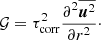
The azimuthally averaged angular momentum in the z direction in spherical polar coordinates is governed by the equation
![Mathematical equation: $$ \begin{aligned}&\frac{\partial }{\partial t} (\overline{\rho } \varpi ^2 \Omega ) + {\boldsymbol{\nabla }}{\boldsymbol{\cdot }}\{\varpi [\varpi \overline{\rho {\boldsymbol{U}}}\Omega + \overline{\rho }\ {Q_{\phi i}} - 2\nu \overline{\rho } \overline{\boldsymbol{\mathsf{S }}}{\boldsymbol{\cdot }}{\hat{\phi }} \nonumber \\&\qquad -\mu _0^{-1}\overline{B}_\phi {\overline{\boldsymbol{B}}} - {M_{\phi i}}] \}=0, \end{aligned} $$](/articles/aa/full_html/2019/02/aa32519-17/aa32519-17-eq5.gif) (2)
(2)
where ρ is the density, ϖ = r sin θ is the lever arm, Ω is the angular velocity, ν is the kinematic viscosity, S is the rate of strain tensor defined below, and  is a unit vector in the azimuthal direction. The velocity and the magnetic field have been decomposed into their mean and fluctuating parts, such that
  and
and  , respectively. In addition to the Reynolds stress defined above, Eq. (2) includes the Maxwell stress
  . Here the correlations of density fluctuations with the velocity have been omitted, which is valid for incompressible flows. In the current study the flows are weakly compressible with Mach number of the order of 0.1, and so this omission should only play a minor role.
In stars, turbulent Reynolds and Maxwell stresses are the main contributors to the angular momentum transport (e.g. Miesch & Toomre 2009; Rüdiger et al. 2013). Much of mean-field theory deals with the task of representing the turbulent correlations in terms of large-scale quantities, as in Eq. (1). Here the relation between the turbulent stress and the large-scale quantities is assumed to be local and instantaneous. Spatial and temporal non-locality are in general non-negligible in turbulent flows (e.g. Brandenburg et al. 2008b; Hubbard & Brandenburg 2009). However, dealing with this generalization will be saved for a future study. The first term on the right-hand side of Eq. (1) describes the Λ effect, or the non-diffusive contribution, to the Reynolds stress in rotating anisotropic turbulence. In addition, a term proportional to large-scale velocities ( ) can also appear on the right-hand side of Eq. (1) (see Frisch et al. 1987). This corresponds to the anisotropic kinetic alpha (AKA) effect which arises in non-Galilean invariant flows (e.g. Frisch et al. 1987; Brandenburg & Rekowski 2001; Käpylä et al. 2018). The forcing used in the present study is Galilean invariant, and thus the contributions from the AKA effect are likely to be negligible. Even so, the current data analysis method cannot detect the AKA effect.
In spherical coordinates the Reynolds stress components  and
and  enter the angular momentum equation directly and correspond to radial and latitudinal fluxes of angular momentum. The third off-diagonal component,
  , contributes to the maintenance of meridional flows and thus influences the angular momentum balance indirectly (e.g. Rüdiger 1989). The non-diffusive part of this stress component, the “meridional” Λ effect, is typically omitted in models of solar and stellar differential rotation. However, numerical simulations indicate that this contribution is non-negligible (Pulkkinen et al. 1993; Rieutord et al. 1994; Käpylä & Brandenburg 2008), and that it may be important in driving the meridional flows in the near-surface layers of the Sun (Hotta et al. 2015; Warnecke et al. 2016). When approximated with an isotropic and homogeneous (constant) turbulent viscosity, the corresponding components of the Λ effect can be formulated as
 (3)
(3)
 (4)
(4)
 (5)
(5)
where νt is the turbulent viscosity, 𝒱 = V sin θ, ℋ = H cos θ, and ℳ = M sin θ cos θ. The factor νtΩ is used for normalization, whereas V, H, and M are dimensionless. These three factors are often expanded in powers of sin2θ (e.g. Brandenburg et al. 1990)
 (6)
(6)
 (7)
(7)
 (8)
(8)
where the dots indicate the possibility of higher-order terms1. We also note that in general the coefficients are functions of position, that is V = V(x), V(i) = V(i)(x), and so on. These coefficients can be written more compactly as
 (9)
(9)
 (10)
(10)
 (11)
(11)
In stellar convection zones, buoyancy drives the convective instability, which can be considered a large-scale anisotropic forcing of turbulence (e.g. Yakhot 1992). This forcing is expected to lead to turbulence dominated by the radial velocity (e.g. Käpylä et al. 2011a). With turbulence of this kind in the slow rotation limit, only the vertical Λ effect is expected to survive. More specifically, the “fundamental” mode of the vertical Λ effect, with the corresponding coefficient V(0), is expected to tend to a constant value, that is V(0) → const. for Ω → 0 (e.g. Rüdiger 1989; Kichatinov & Rüdiger 1993). A corresponding horizontal effect, described by H(0), does not arise in the hydrodynamic case because it would require another preferred direction to be present in the system (Rüdiger 1989). Large-scale magnetic fields can provide this additional anisotropy in which case H(0) ≠ 0 (Kitchatinov et al. 1994b). The higher-order components of the vertical and horizontal Λ coefficients are expected to be proportional to higher (even) powers of Ω due to the symmetry properties of Λijk (Rüdiger 1989; Rüdiger et al. 2014). The theory of the meridional Λ effect is much less well developed2.
2.2. Observational evidence
Traditionally the most often used argument in favour of the existence of the Λ effect has been the observed cross-correlation of horizontal proper motions of sunspots, which have been interpreted as the Qθϕ component of the Reynolds stress (e.g. Ward 1965; Pulkkinen & Tuominen 1998). These studies yield a value of the order of 103 m2 s−1 which is positive (negative) in the northern (southern) hemisphere of the Sun. If the Reynolds stress is assumed to result from the shear stress alone (Boussinesq ansatz),
 (12)
(12)
the Qθϕ component in spherical coordinates is
 (13)
(13)
This implies that νt < 0 given that sin θ > 0 and  in the northern hemisphere of the Sun (see the discussions in Tuominen & Rüdiger 1989; Pulkkinen et al. 1993). A more recent result from giant cells, obtained from supergranulation tracking, suggests the same sign but two orders of magnitude lower amplitude for Qθϕ (Hathaway et al. 2013). Although a negative νt has been reported to occur in certain cases of two-dimensional turbulence (e.g. Krause & Rüdiger 1974), there is no evidence for νt < 0 for more general three-dimensional flows. Negative turbulent viscosity would also lead to a pile-up of energy at small scales which is considered unphysical. A more plausible explanation is that Eq. (13) is incomplete and that a non-diffusive term (Λ effect) has to be present. In this case, a positive Qθϕ in the northern hemisphere can occur when the rotational influence on the flow is sufficiently large, such that the contribution of the Λ effect to the Reynolds stress dominates over that from turbulent viscosity (Rüdiger et al. 2014). Thus, sunspots and giant cells are likely to probe these deeper, and more rotationally constrained, parts of the convection zone. However, due to the vanishing horizontal Λ effect near the surface (Rüdiger et al. 2014), the viscous term, Eq. (12), is expected to dominate there and to produce a negative Qθϕ. This detection from helioseismology of supergranulation has been reported recently by Hanasoge et al. (2016).
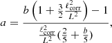
On the other hand, near the solar surface, where the rotational influence is weak (e.g. Greer et al. 2015, 2016), only the fundamental mode of the Λ effect is expected to be non-zero. This coincides with the near-surface shear layer where the angular velocity has a uniform radial gradient of Ω independent of latitude (Barekat et al. 2014). This can be explained with a simple model where the meridional flows are neglected and where only the fundamental mode of the Λ effect is taken into account (e.g. Gailitis & Rüdiger 1982; Kitchatinov 2016), yielding
 (14)
(14)
where the latter is the observational result of Barekat et al. (2014). No direct observational data for the behaviour of Qrϕ in the deep parts or of Qrθ anywhere in the solar convection zone are currently available. Using a combination of theoretical arguments and helioseismic measurements, Miesch & Hindman (2011) infer that the radial angular momentum transport attributed to turbulent convection in the near-surface shear layer is radially inward. The Boussinesq ansatz,  , would again imply νt < 0 in the absence of a radial Λ effect.
3. Model
Compressible turbulent fluid flow is modelled in a triply periodic cube with or without magnetic fields. The gas is assumed to obey an isothermal equation of state  , where p is the pressure and cs is the constant speed of sound. Gravity is neglected for simplicity as it would necessarily introduce inhomogeneity in a compressible system, and because the minimal requirements for the appearance of the Λ effect can be achieved by a homogeneous forcing. The system is governed by the induction, continuity, and Navier–Stokes equations
![Mathematical equation: $$ \begin{aligned}&\frac{\partial {\boldsymbol{A}}}{\partial t} = {\boldsymbol{U}}\times [ {\boldsymbol{B}} + {\boldsymbol{B}}^{(0)}] - \eta \mu _0{\boldsymbol{J}}, \end{aligned} $$](/articles/aa/full_html/2019/02/aa32519-17/aa32519-17-eq29.gif) (15)
(15)
 (16)
(16)
 (17)
(17)
where A is the magnetic vector potential, U is the velocity, B = ∇ × A is the magnetic field, B(0) is the uniform imposed external magnetic field, η is the magnetic diffusivity, μ0 is the permeability of vacuum,  is the current density, D/Dt = ∂/∂t − U⋅∇ is the advective time derivative, ρ is the density, Ω is the rotation vector, and Fvisc and Fforce respectively describe the viscous force and external forcing.
The viscous force reads
 (18)
(18)
where ν is the constant kinematic viscosity and  is the traceless rate of strain tensor where the commas denote differentiation.
The external forcing is given by
![Mathematical equation: $$ \begin{aligned} {\boldsymbol{F}}^\mathrm{force}({\boldsymbol{x}},t) = \mathrm{Re}\{{\boldsymbol{\mathsf{N }}}{\boldsymbol{\cdot }}{\boldsymbol{f}}_{{\boldsymbol{k}}(t)} \exp [\mathrm{i} {\boldsymbol{k}}(t){\boldsymbol{\cdot }} {\boldsymbol{x}} - \mathrm{i}\phi (t)]\}, \end{aligned} $$](/articles/aa/full_html/2019/02/aa32519-17/aa32519-17-eq35.gif) (19)
(19)
where x is the position vector and N = fcs(kcs/δt)1/2 is a tensorial normalization factor. Here f contains the non-dimensional amplitudes of the forcing (see below), k = |k|, δt is the length of the time step, and −π < ϕ(t) < π is a random delta-correlated phase. The vector fk describes non-helical transversal waves, and is given by
 (20)
(20)
where  is an arbitrary unit vector, and where the wavenumber k is randomly chosen. The PENCIL CODE3 was used to produce the numerical simulations.
3.1. Units and system parameters
The units of length, time, density, and magnetic field are
![Mathematical equation: $$ \begin{aligned}[x] = k_1^{-1}, [t]=({c_{\rm s}} k_1)^{-1}, [\rho ] = \rho _0, [B] = \sqrt{\mu _0\rho _0} c_{\rm s}, \end{aligned} $$](/articles/aa/full_html/2019/02/aa32519-17/aa32519-17-eq38.gif) (21)
(21)
where ρ0 is the initially uniform value of density. The forcing amplitude is given by
 (22)
(22)
where f0 and f1 are the amplitudes of the isotropic and anisotropic parts, respectively. Furthermore, δij is the Kronecker delta, and Θk is the angle between the vertical direction and k. The forcing wavenumber is chosen from a narrow range 9.9 ≤ kf/k1 ≤ 10.1. The set of wavenumbers consists of 318 unique combinations of k = (kx, ky, kz), which are uniformly distributed (for more details about the forcing, see Brandenburg 2001). The amplitude of the forcing is chosen such that the Mach number, Ma = urms/cs, where urms is the volume-averaged rms velocity, is of the order of 0.1.
The remaining system parameters in the hydrodynamic cases are the kinematic viscosity ν, and the rotation vector Ω = Ω0(−sin θ, 0, cos θ)T, where θ is the angle that the rotation vector makes with the vertical (z) direction. An angle of θ = 0 (90°) corresponds to the north pole (equator). Viscosity and rotation can be combined into the Taylor number
 (23)
(23)
where Ld = 2π/k1 corresponds to the size of the computational domain and where k1 is the wavenumber corresponding to the box size.
In magnetohydrodynamic (MHD) cases the magnetic diffusivity is an additional control parameter. This is quantified by the magnetic Prandtl number, which is the ratio of the kinematic viscosity and magnetic diffusivity:
 (24)
(24)
All of the simulations in the present study use Pm =1. The imposed magnetic field strength is measured by the Lundquist number
 (25)
(25)
where vA = B0/( μ0ρ0) is the Alfvén speed and B0 is the amplitude of the imposed field. The choice of a purely toroidal imposed field comes from turbulent mean-field models of the solar dynamo (e.g. Käpylä et al. 2006; Pipin & Kosovichev 2013) and three-dimensional global simulations which suggest that the strong differential rotation produces a dominant toroidal field in the bulk of the convection zone (e.g. Ghizaru et al. 2010; Käpylä et al. 2012; Nelson et al. 2013).
3.2. Diagnostics quantities
The following quantities are outcomes of the simulations that can only be determined a posteriori. The fluid and magnetic Reynolds numbers are given by
 (26)
(26)
The rotational influence on the flow is quantified by the Coriolis number based on the forcing scale
 (27)
(27)
where ℓ = Ldk1/kf = 2π/kf. The Strouhal number is given by
 (28)
(28)
where τ is the correlation time of the flow.
The magnetic field strength is often quoted in terms of the equipartition value
 (29)
(29)
Finally, the parameters
 (30)
(30)
characterize the vertical and horizontal anisotropy of turbulence.
3.3. Modelling and data analysis strategies
Numerous sets of simulations were performed where a single physical ingredient (rotation, imposed magnetic field, viscosity) was varied and the other system parameters were kept fixed. In most cases each set of simulations consisted of ten runs in which the colatitude θ was varied in steps of 10° from the north pole to the equator. The only exceptions to this are Sets AI1–AI4 and AI1h, which were done at a fixed colatitude of θ = 45°. The simulations are summarized in Tables 1–4. The grid resolution of the bulk of the simulations is low (1443) in order to cover large parameter ranges with a reasonable computational cost. Higher resolutions were used in cases with a larger scale-separation ratio (Set AI1h) and in those cases with a higher Reynolds number (Sets RE7 and RE8).
Summary of runs with varying rotation and turbulence anisotropy at θ = 45°.
Summary of runs with varying Ω⋆.
Summary of runs where Re was varied.
Summary of runs with magnetic fields.
The simulations were made in the f–plane approximation in Cartesian coordinates. For the off-diagonal Reynolds stresses this means moving from spherical polar coordinates to local Cartesian ones, implying (r, θ, ϕ)→(z, x, y). Combining this with Eqs. (3)–(11) and Eq. (27), and using the estimate  for the turbulent viscosity (Kitchatinov et al. 1994a), yields
 (31)
(31)
 (32)
(32)
 (33)
(33)
where the tilde refers to normalization by  , and where
 (34)
(34)
Furthermore, in the local domain approximation in the absence of gravity the coefficients 𝒱, ℋ, and ℳ are independent of position. It is useful to parameterize the Reynolds stress in terms of the coefficients Eqs. (6)–(8) to make the results more readily comparable with theory and usable in mean-field modelling. The numerical data from Eqs. (31)–(33) is thus fitted with Eqs. (9)–(11) with varying number of terms included. The issues related to fitting (Sect. 1) are alleviated by the fact that no large scale flows are present in the current simulations, and the off-diagonal components of the Reynolds stress can be considered to arise solely due to the Λ effect. However, the choice of the θ-dependence of the fit for the coefficients V(i), H(i), and M(i) still leads to non-uniqueness of the extracted coefficients.
The following procedure was used in the present study: the coefficients V(i), H(i), and M(i) were obtained from fits to Eqs. (9)–(11) for each set of simulations corresponding to a fixed Taylor number. Three criteria were considered in evaluating the adequacy of the fit:
-
The fit is considered acceptable if the rms deviation of the fit from the numerical data,
![Mathematical equation: $$ \begin{aligned} \delta {Q_{ij}^\mathrm{fit}}=\sqrt{\frac{1}{N+1}\sum \limits _{k=1}^N \left[{Q_{ij}^\mathrm{fit}}(\theta _k) - {Q_{ij}}(\theta _k) \right]^2}, \end{aligned} $$](/articles/aa/full_html/2019/02/aa32519-17/aa32519-17-eq58.gif) (35)
(35)is smaller than the rms error of the data
![Mathematical equation: $$ \begin{aligned} \delta {Q_{ij}^\mathrm{data}}=\sqrt{\frac{1}{N+1}\sum \limits _{k=1}^N \left[\delta {Q_{ij}^\mathrm{data}}(\theta _k)\right]^2}, \end{aligned} $$](/articles/aa/full_html/2019/02/aa32519-17/aa32519-17-eq59.gif) (36)
(36)where N + 1 = 10 is the number of data points in each set, θk = k ⋅ 10°, and where
 are the errors of the individual data points. The latter were computed by dividing the time series in three parts and averaging over each part. The greatest deviation of these from the average over the full data set was taken to represent the error.
 -
Independent from criterion 1, an additional constraint is imposed on
 : the expansions in Eqs. (9)–(11) are truncated if an additional term does not decrease
  by more than 10%.
 -
In some cases, when the latitudinal profile of the stress changes as a function of Ω⋆, equally good fits may be found for a higher- and lower-order expansion. In these cases, the higher-order term was taken into account if it made the Ω⋆ dependence of the coefficient smoother.
In practice, Criterion 1 cannot be fulfilled on many occasions. In these cases, Criterion 2 becomes decisive, as is demonstrated in the left and middle panels on the lower row of Fig. 2. Criterion 3 was invoked twice: in Set E the fits with ℋ(1) and ℋ(2), and ℳ(1) and ℳ(2), respectively, were roughly equally good but the latter choices lead to a smoother rotational dependence of H(i) and M(i) (see Sect. 4.3.1).
Once a higher-order term in the expansion is included, it is retained for all subsequent sets at higher Taylor numbers. Examples of the different fits are shown for a representative selection of runs in Fig. 1, where the solid lines indicate the accepted fit according to the procedure outlined above and the dotted lines indicate discarded fits.
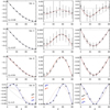 |
Fig. 1. From left to right panels: 𝒱, ℋ, and ℳ from Eqs. (31)–(33), along with the fits to Eqs. (9)–(11) where one (black), two (red), or three (blue) first terms of the expansions are retained. Data from Sets A (top row), C, E, and H (bottom panel). |
4. Results
4.1. Reynolds stress in the slow rotation limit
Quasi-linear theory of the Λ effect predicts that for vertically dominated turbulence only the fundamental mode of the vertical Λ effect, corresponding to V(0) in Eq. (6), is present in the limit of slow rotation (Rüdiger 1989; Kichatinov & Rüdiger 1993). This implies that vertical Reynolds stress is linearly proportional to Ω in this regime, or
 (37)
(37)
The other off-diagonal components are predicted to be at least second order in Ω (Rüdiger 1989). The theoretical predictions are tested by five sets of simulations where θ = 45° is fixed and the rotation rate is varied such that the Coriolis number covers the range 0.01…0.47 (see Table 1).
Figure 2 shows that the horizontal stress Qxy is positive and the meridional stress Qxz is negative, indicating H > 0 and M < 0, respectively. The numerical results are consistent with the analytic results of Rüdiger (1989), that is  and
and  . However, due to the relatively large error of
  , it is also compatible with an
  -dependence. The magnitude of the horizontal stress in this parameter regime is
  and the error estimates are substantial, although the simulations with the smallest Taylor numbers were integrated for several tens of thousands eddy turnover times. This is due to the fact that in the slow rotation limit the horizontal Λ effect is proportional to AH (Rüdiger 1980), which is rotation-induced and which remains small in comparison to AV in this regime (see Table 1). It is noteworthy that the meridional stress Qxz has a clearly greater magnitude in comparison to Qxy. This is due to the stronger Ω⋆ dependence of the latter (Rüdiger 1989). The vertical stress Qyz is significantly stronger than the other two components and shows a linear dependence on Co in accordance with the theoretical prediction (see Fig. 2c).
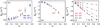 |
Fig. 2. Normalized Reynolds stress components Qxy, Qxz, and Qyz, panels a–c, respectively, from θ = 45° as functions of Ω⋆. In panels a and b data from Sets AI1 and AI1h is shown, whereas in panel c additional data from Sets AI2–4 is included. The dotted lines in panel c are proportional to AVΩ⋆. |
4.2. Dependence of ΛV on turbulence anisotropy
The Λ effect depends not only on rotation, but also on the properties of turbulence (Rüdiger 1989). More specifically, analytic theories predict that the anisotropy of turbulence plays a crucial role (Rüdiger 1980, 1989). Here the rotation-induced Reynolds stress is estimated from the Navier-Stokes equations using a minimal τ approach (for a more complete derivation, see Käpylä & Brandenburg 2008). The time derivative of the Reynolds stress is given by
 (38)
(38)
where
 (39)
(39)
where Ni encompasses viscous and non-linear terms. Using Eq. (39) in Eq. (38) yields
 (40)
(40)
where 𝒯ij contains triple and higher-order correlations. Assuming a stationary state with  , and approximating the triple correlations as 𝒯ij = −Qij/τ in accordance with the τ approximation (e.g. Blackman & Field 2002, 2003), where τ is a relaxation time, gives
 (41)
(41)
Numerical simulations of turbulent passive scalar and magnetic field transport have yielded support for the validity of the τ approximation (e.g. Brandenburg et al. 2004; Brandenburg & Subramanian 2005b; Snellman et al. 2012). However, one must bear in mind that this is a rather simplistic approach to the turbulence closure problem and that the results should not be considered exact. Associating this with the Λ effect, that is assuming  , the vertical (yz) component of the stress is
 (42)
(42)
The last term on the right-hand side can be omitted in the slow rotation limit where |Qxz|≪|Qzz − Qyy|. Furthermore, the relaxation time can be related to the turnover time ℓ/urms via τ = Stℓ/urms, where St is the Strouhal number. Inserting this into Eq. (42) and dividing by  yields
 (43)
(43)
Four sets of simulations (Sets AI1–4) were made where the anisotropy of the turbulence was systematically reduced in comparison to the maximum case by reducing the ratio of the forcing amplitudes f1/f0. Set AI1h has otherwise similar parameters to those of AI1, but was done with forcing wavenumber  (see Table 1). The runs in Sets AI2–4 were not integrated as long as those in Sets AI1 and AI1h, leading to poor convergence of the stress components Qxy and Qxz. Thus, these results are not shown here. The vertical stress Qyz is shown as a function of Ω⋆ from Sets AI1–4 in Fig. 2c. The numerical results indicate that the stress, and thus the vertical Λ effect, is linearly proportional to the turbulence anisotropy in the slow rotation regime. Comparison of the stress with Eq. (43) shows good agreement for all sets of runs with St =0.13.
4.3. Reynolds stress and Λ effect as functions of rotation
In a stellar convective envelope the rotational influence on the flow can vary by several orders of magnitude as a function of radius due to the strong density stratification. This can be seen from the Coriolis number for the Sun
 (44)
(44)
where Ω⊙ = 2.7 × 10⁻⁶ s−1 is the mean solar rotation rate, τ = Hp/uconv is an estimate convective turnover time, Hp = −(∂lnp/∂r)−1 is the pressure scale height, and uconv is the convective rms-velocity. Mixing length models of the solar convection zone (e.g. Stix 2002) yield values of uconv and Hp such that Co⊙ ranges from 10−3 in the photosphere to roughly unity at r = 0.95R⊙, while reaching values of more than ten at the base of the CZ (e.g. Käpylä et al. 2005). At least this range in Coriolis numbers needs to be probed for the results to be usable in mean-field models of solar and stellar differential rotation.
4.3.1. Latitudinal dependence of the Reynolds stress
The runs probing the rotation dependence are listed in Table 2. The Reynolds numbers in these runs are relatively modest4 (Re =5.5…24). However, the Reynolds number is the ratio of the viscous (τν) to turbulent turnover (τu) times, that is  . Thus, the viscous timescale is always significantly longer than the characteristic flow timescale in the current simulations. The values of Ω⋆ in Sets A–I range from 0.09 to 9, which roughly corresponds to the range expected in the solar convection zone. However, for the fiducial value of the Reynolds number (Re =14), the flow develops a large-scale vortex at θ = 0 when the Taylor number is increased from 1.56 × 10⁹ to 6.23 × 10⁹ corresponding to 4.5 ≲ Ω⋆ ≲ 9.0 (see Fig. 3). Similar vortices have been obtained in the rapid rotation regime in other settings where the turbulence is driven either by compressible or Boussinesq convection (e.g. Chan 2003, 2007; Käpylä et al. 2011c; Guervilly et al. 2014; Rubio et al. 2014) or isotropic forcing similar to the current study (e.g. Biferale et al. 2016). These structures dominate the flow in the statistically saturated state which explains the extreme values of AV, H, Ω⋆, and Re in Set I (see Table 2). In cases where the rotation vector is inclined with the direction of anisotropy, mesoscale flow structures with modes such as (kx, ky, 0)=(3, 0, 0) for Uy appear. Similar structures also dominate the Reynolds stress and overwhelm the turbulent contributions. Thus, Set I is disregarded from further analysis and higher rotation rates were not explored with Re =14. Instead, a series of runs were made with Re =5.5 (Sets AA–GG in Table 2), roughly overlapping with Sets D–H, to study the rapid rotation regime. Vortices do not appear in these runs even at substantially higher rotation rates (up to Ω⋆ ≈ 45). This is consistent with the finding of Käpylä et al. (2011c) that a critical Reynolds number has to be exceeded for the vortices to form. The study of large-scale vorticity generation and its effects on angular momentum transport will be presented elsewhere.
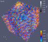 |
Fig. 3. Vertical component of vorticity ωz = (∇ × U)z in units of csk1 (colour contours) and flow vectors (black and white streamlines) in terms of the local Mach number Ma = |u|/cs from Run I0. |
Figure 4 shows the off-diagonal stresses Qyz, Qxy, and Qxz from a representative selection of runs. In the case of slowest rotation (Set A, Ω⋆ = 0.09), the horizontal stress Qxy is not statistically significant, whereas the meridional stress Qxz is barely so (see also Fig. 1). The vertical stress Qyz is well-defined due to the strong anisotropy of the turbulence already at the lowest rotation rate considered here. At more rapid rotations the horizontal (meridional) stress acquires consistently positive (negative) values at all latitudes (Set E with Ω⋆ = 0.91; Fig. 4b). The latitude at which the horizontal and meridional stresses peak shifts toward the equator as a function of Ω⋆. In the regime of rapid rotation, the maximum of Qxy continues to move to lower latitudes, but this trend is not as extreme as in local simulations of rapidly rotating convection (e.g. Käpylä et al. 2004; Rüdiger et al. 2005; Hupfer et al. 2005). The reason is that in convection simulations large-scale flow structures, also known as banana cells (Busse 1970), develop near the equator and enhance the horizontal stress (Käpylä et al. 2011b). However, such flow structures are absent in the current simplified models. In Sets FF and GG, with Ω⋆ = 23 and 45, Qxy shows indications of a sign change at high latitudes, which was not found by Käpylä & Brandenburg (2008)5. The meridional stress Qxz reaches a maximum around θ = 45° at intermediate rotation (Ω⋆ = 0.5…10) and no clear sign change is observed even at higher Ω⋆. Also, this differs from the results of Käpylä & Brandenburg (2008) where a sign change occurred near the equator for Ω⋆ ≈ 34 in the current units. In the most rapidly rotating runs (Set GG), some indication of a sign change at high latitudes is present. Formally, the differences of the current Sets A–I to the runs of Käpylä & Brandenburg (2008) are minor: the grid resolution is roughly twice as high in the current simulations, and the forcing is applied at  instead of
  . Finally, the Mach number is roughly a factor of three smaller in the current simulations. It is unclear which of the differences is causing the results to diverge at rapid rotation. The results at slow and intermediate rotation (0.09 ≲ Ω⋆ ≲ 20) are, however, in good agreement with those of Käpylä & Brandenburg (2008).
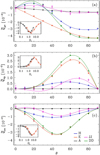 |
Fig. 4. Off-diagonal stresses from a representative set of runs. Diamonds: normalized Reynolds stress components |


The vertical stress Qyz is clearly the dominant component in the current models. In the slow rotation regime it shows a stable configuration such that the values are consistently negative, and the latitude dependence experiences only minor changes until around Ω⋆ ≈ 0.9 (see Fig. 4). This is consistent with theory of the vertical Λ effect at slow rotation (Rüdiger 1989). In the rapid rotation regime a sign change occurs at high latitudes and the magnitude is drastically reduced near the equator in accordance with the results of Käpylä & Brandenburg (2008; see the inset in Fig. 4a). A low latitude sign change of the vertical stress is not observed in contrast to local and global convection simulations where also the vertical turbulence anisotropy changes sign (e.g. Käpylä et al. 2004, 2014). The magnitudes of both Qxy and Qxz increase until Ω⋆ ≈ 5 with the latter being somewhat larger at all rotation rates (see the insets in Figs. 4b and c). The decrease in the stress at rapid rotation is associated with rotational quenching of the Λ effect (Kichatinov & Rüdiger 1993), which is likely due to the reduced anisotropy in that regime (see Table 2). Differences with convection simulations may be explained by the missing contributions from the heat flux in the present models (Kleeorin & Rogachevskii 2006).
4.3.2. Parameterization in terms of the Λ effect
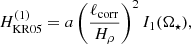
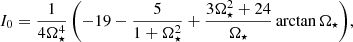
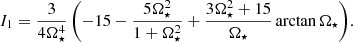
The procedure outlined in Sect. 3.3 was used to extract the coefficients pertaining to the Λ effect. Figure 5 shows the results obtained from Sets A–H and AA–GG. The fundamental mode of the Λ effect is recovered in the slow rotation limit (Ω⋆ ≲ 0.5), manifested by V(0) tending to a constant value of ≈ − 0.5 with V(1) and V(2) being negligible. The vertical stress is well described by V(0) until Ω⋆ ≈ 1, beyond which the higher-order components are needed. In the fits obtained, V(1) and V(2) have different signs with the former having roughly twice the absolute magnitude of the latter. Reasonable agreement is found between the overlapping sets of runs with different values of Re (Sets D–H and AA–DD) in the regime of intermediate rotation (0.5 ≲ Ω⋆ ≲ 5). In the rapid rotation regime all of the V(i) coefficients are quenched and tend to almost zero at the highest value of Ω⋆. The value of V(0) found in the slow rotation regime is almost exactly half that indicated by helioseismology (Barekat et al. 2014). The current results, however, depend crucially on the adopted value of νt, see Eqs. (31)–(34). By using  (e.g. Rüdiger 1989), the observational result V(0) ≈ −1 would be recovered. This highlights the arbitrariness of the choice of νt and the need for methods to estimate it independently.
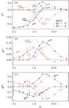 |
Fig. 5. Coefficients V(i), H(i), and M(i) as functions of Ω⋆ from Sets A–H (solid lines) and AA–GG (dashed). The dash-dotted lines in panel a and panel b correspond to analytic results Eqs. (45) and (46) as indicated by the legends. Here a = 1.75 was used to match |

The coefficients H(1) and H(2), corresponding to the horizontal Λ effect, are always positive in Sets A–H. The results from Sets AA–CC agree qualitatively with the higher-Re runs although the values are generally lower. This is due to the fact that the coefficients are not yet in an asymptotic regime with respect to the Reynolds number (see Sect. 4.4 and Fig. 6). In the lower-Re runs H(1) turns negative around Ω⋆ ≈ 11. For Ω⋆ ≳ 5 a strong rotational quenching is observed and the H(i) coefficients also tend to very small values at the highest rotation rates corresponding to Ω⋆ = 23 and 45.
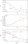 |
Fig. 6. Coefficients pertaining to the Λ effect as functions of Re: V(0) (panel a), H(1) (panel b), and M(0, 1) (panel c) for Sets RE1–RE8 with Ω⋆ = 1.0 and AV ≈ −0.3. The dashed lines are proportional to Re. |
The hitherto poorly studied meridional Λ coefficients are shown in Fig. 5c). The simple cos θ sin θ dependence of the stress is well described by M(0) alone at slow rotation (Ω⋆ ≲ 0.5). For Ω⋆ ≳ 0.5, this behaviour gives way to a stronger concentration at mid-latitudes. This is manifested by a diminishing M(0) with increasing M(1) and M(2) with almost equal absolute magnitudes but opposite signs for Ω⋆ ≳ 1. As with the vertical and horizontal Λ effects, a strong rotational quenching is observed for Ω⋆ ≳ 5. The correspondence between the lower and higher Reynolds number runs is again reasonably good.
4.3.3. Comparison to analytic results
In the studies of Kitchatinov (2004) and Kitchatinov & Rüdiger (2005) a distinction is made between the contributions from density stratification and anisotropy of turbulence to the Λ effect. The latter is dominant in the slowly rotating regime which corresponds to the upper layers of the solar convection zone and the current simulations. The analytic model of Kitchatinov & Rüdiger (2005) predicts the following functional forms for V(0) and H(1) (with V(1) = H(1)) in the case where the Λ effect is solely due to turbulence anisotropy
 (45)
(45)
 (46)
(46)
where a is an anisotropy parameter (see below), ℓcorr is the correlation length of turbulence, and Hρ = −(∂lnρ/∂r)−1 is the density scale height. The correlation length ℓcorr is taken to equal the mixing length by Kitchatinov (2004) and Kitchatinov & Rüdiger (2005), that is ℓcorr = αMLTHp, where αMLT = 1.7 is the mixing length parameter and Hp is the pressure scale height. In the present case ℓcorr is taken to correspond to the forcing scale of turbulence ℓ = 2π/kf, but no scale corresponding to Hρ can be identified due to the homogeneity of the system under consideration. Furthermore, Hρ = Ld is assumed for simplicity. The quenching functions I0 and I1 are given by
 (47)
(47)
 (48)
(48)
The analytic results  and
and  are compared with the numerically obtained coefficients V(i) and H(1) in Fig. 5. The analytic and numerical results are in rough qualitative agreement for slow rotation (Co ≲ 1), but several differences are immediately apparent. First, the numerical data is at odds with the analytic result indicating that V(1) = H(1). An obvious candidate for the discrepancy is that the numerical values are obtained by fitting where V(1) and H(1) are considered independent. The second major difference is that the numerical data for sufficiently rapid rotation (Ω⋆ ≳ 1) is incompatible with expressions of V and H which consider only terms proportional to sin2θ.
Furthermore, in the foregoing analysis the anisotropy parameter a was kept as a free parameter and tuned such that  in the slow rotation limit. It is also possible to compute a directly using Eq. (A14) in Appendix A of Kitchatinov & Rüdiger (2005) by substituting
  and
and  , and defining
  :
:
 (49)
(49)
where L is a length scale corresponding to large-scale inhomogeneity. Assuming L = Ld and ℓcorr = ℓ gives ℓcorr/Ld = ℓ/L = k1/kf ≈ 0.1, allowing Eq. (49) to be solved with b as an input from simulations. The maximum anisotropy used in the bulk of the simulations is AV ≈ 0.52, which yields b ≈ 2.1 and a ≈ 2.7. This is somewhat greater than the values used in the fitting above. However, this discrepancy is mostly due to the freedom in choosing the value of νt.
4.4. Dependence of Λ effect on Reynolds number
The simulations in the preceding sections were made at low Reynolds numbers in comparison to the astrophysically relevant regime. Figure 6 shows the Λ coefficients for a representative case where the Coriolis number (Ω⋆ ≈ 1.0) and turbulence anisotropy (AV ≈ 0.3) were fixed in the range Re ≈ 0.6…99. The Coriolis number was chosen such that the higher-order coefficients V(1), V(2), H(2), and M(2) did not appear according to the criteria in Sect. 3.3. At low Reynolds numbers Re = 0.6…2 all of the coefficients are proportional to Re as expected from mean-field theory. At low Re the error bars for H(1) and M(0, 1) increase because the mean values of Qxy and Qxz are small. Furthermore, the coefficients level off beyond Re ≳ 10 where they are consistent with constants although with large error bars in particular for H(1). These results suggest that the results obtained at Re ≈10 are representative of what can be expected in more turbulent cases.
4.5. Influence of large-scale magnetic fields
Dynamically significant magnetic fields are ubiquitous in astrophysical objects where the Λ effect is thought to be important. In particular, stars with convection zones harbour dynamos that produce magnetic fields on various scales. The effects of large-scale magnetic fields on the Λ effect have been studied analytically by Kitchatinov et al. (1994b) and Kitchatinov (2016). These studies indicate that large-scale magnetic fields tend to quench the Λ effect, but also that an additional H(0) effect arises in the presence of a horizontal mean magnetic field. Here the study of Kitchatinov et al. (1994b) is followed where the quenching formulae for V(0) and H(0) were calculated as functions of the magnetic field assuming the field to be horizontal. They found that
 (50)
(50)
 (51)
(51)
where
 (52)
(52)
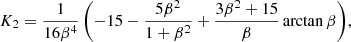 (53)
(53)
β = B0/Beq, and
 (54)
(54)
These equations correspond to the case where the anisotropy is due to the density stratification and where 𝒢 is describing this. These equations indicate that V(0) is monotonically quenched by magnetic fields, whereas H(0) vanishes as β → 0 and obtains a maximum for β ≈ 0.94. Direct comparison to the analytic study is not possible since the turbulence intensity is homogeneous in the current simulations. Thus, 𝒢 is treated here as a free parameter.
Here the dependence of the Λ effect on large-scale magnetic fields is studied systematically with controlled numerical experiments, where either a uniform horizontal (Sets LSFH1-9) or a vertical (Sets LSFV1-9) large-scale imposed magnetic field is present (see Table 4). The magnetic Reynolds number (ReM ≈ 14) is chosen such that it does not exceed the critical value ReM ≈ 30 for a small-scale dynamo to be excited (Brandenburg 2001). The same analysis as above in the hydrodynamic case is performed on the total turbulent stress,
 (55)
(55)
where  is the Maxwell stress. In the current fully periodic and homogeneous case no large-scale magnetic fields, apart from the imposed field
  , are present. Lundquist numbers ranging from 0.1 to 50 are studied for both field geometries (see Table 4). This range corresponds to 7 × 10⁻³…3.5 in terms of the equipartition strength Beq.
The Λ coefficients obtained from the numerical models are shown in Fig. 7. The effect of the large-scale magnetic field begins to be noticeable for Lu = 1 corresponding to roughly 0.1Beq, although M(1) and M(2) are affected already by weaker fields. For stronger fields the magnitude of all coefficients, except H(0) in the runs with a horizontal field, start to decrease. The existence of a non-zero H(0) was predicted analytically by Kitchatinov et al. (1994b) and the current simulations confirm this finding numerically for the first time. This part of the Λ effect arises not only due to a negative contribution from the Maxwell stress, but also from a gradual sign change of the Reynolds stress starting from the poles (see Fig. 8). In the case of the strongest imposed field (Set LSFH9 with β ≈ 3.5) the horizontal stress is negative at all latitudes apart from the equator. In reality, the stress must vanish at the poles because  in spherical polar coordinates (corresponding to
  in the current coordinates) also vanishes. The analytic results, where 𝒢 is tuned to match the numerical results of V(0) at β = 0 and the maximum amplitude of H(0), are shown alongside the numerical results in Fig. 7.
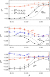 |
Fig. 7. Coefficients V(i) (panel a), H(i) (panel b), and M(i) (panel c) as functions of β. Solid (dashed) lines correspond to runs with an imposed horizontal (vertical) field. The dotted horizontal line denotes the zero level. The open circles on the left axis indicate the hydrodynamic values from Set E. The dash-dotted lines show analytic results according to Eq. (50) (panel a) and Eq. (51) (panel b). |
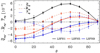 |
Fig. 8. Normalized horizontal (xy), Reynolds (dashed), Maxwell (dash-dotted), and total (thick solid) stress from Sets LSFH1 (black), LSFH5 (red), and LSFH9 (blue) as functions of θ. |
Significant magnetic quenching is apparent for all coefficients except H(0) clearly before equipartition strength is reached. The behaviour of the Λ coefficients is similar in the vertical and horizontal field cases (compare the solid and dashed lines in Fig. 7). However, noticeable quenching occurs at somewhat lower magnetic field strengths in the LSFV runs. The analytic and numerical results show qualitatively similar behaviour. The magnetic quenching occurs at somewhat lower magnetic fields in the simulations in comparison to theory. For magnetic fields near equipartition, the Λ coefficients have diminished to roughly 10–20% of their hydrodynamic values. The absolute maximum value for H(0) is obtained for Lu = 10 (Set LSFH7) corresponding to B0 ≈ 0.8Beq, after which its magnitude also decreases. This is somewhat lower than the analytically predicted value of β ≈ 0.94. The apparently deviating behaviour, i.e. increasing magnitude for β ≳ 0.3 of V(1), H(2), and M(0), is due to the change in latitude distribution of the stress as a function of  . The magnetic quenching comes about because the Maxwell stress has a similar latitude distribution, but is of opposite sign to the Reynolds stress. Moreover, the Maxwell stress increases monotonically as a function of the imposed magnetic field (see Fig. 9). However, the Reynolds stress also increases for β ≳ 1. The tendency of the Reynolds and Maxwell contributions to cancel is reminiscent of the behaviour of the total turbulent stress in semi-global convection simulations where small- and large-scale dynamos are simultaneously excited (Käpylä et al. 2017).
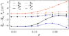 |
Fig. 9. Normalized vertical (yz, solid) and meridional (xz, dashed) Reynolds (blue), Maxwell (red), and total (thick black) stresses as functions of the normalized magnetic field strength β. Data from θ = 90° (50°) for the vertical (meridional) stress is shown. |
5. Conclusions
The non-diffusive contribution to the Reynolds stress, or the Λ effect, from numerical simulations of homogeneous anisotropically forced turbulence was found to agree with analytic theory derived under the second-order correlation approximation. This includes the scaling of the off-diagonal Reynolds stress for slow rotation and the proportionality of the vertical Λ on the vertical turbulence anisotropy AV. Furthermore, the Reynolds stress is proportional to the Reynolds number at low Re. At more rapid rotation (Ω⋆ ≳ 1) the numerical results indicate more complex latitude dependences than predicted by theory. This entails a higher than second power of sin θ for adequate fits of the data. At rapid rotation (Ω⋆ ≳ 3…5 depending on the stress component), a strong rotational quenching was observed. This quenching is predicted by theory (e.g. Kichatinov & Rüdiger 1993; Kitchatinov & Rüdiger 2005), but occurs at more rapid rotation in the simulations.
The bulk of the current results are restricted to low values of the Reynolds number (Re =6…14). Current results indicate that the Reynolds stress and the deduced Λ effect become independent of Re between 10 < Re < 20 at slow rotation. At rapid rotation the system develops large-scale flows in the form of vortices that have a profound influence on the dynamics. Such vortices are ubiquitous in rapidly rotating turbulent systems (e.g. Yeung & Zhou 1998; Chan 2003; Favier et al. 2014) at sufficiently rapid rotation and Reynolds numbers. Thus it would appear to be logical to assume that large-scale vortices would dominate the dynamics in rapidly rotating astrophysical objects where the Reynolds numbers are much higher than in the current simulations. However, the vortices are also known to turn into jets in systems with horizontal aspect ratios unequal to one (Guervilly & Hughes 2017) and to promote large-scale dynamo action (Bushby et al. 2018). Strong magnetic fields, however, can also quench the vortices (Käpylä et al. 2013).
A strong quenching of the Λ effect was found in the case where an imposed vertical or horizontal uniform magnetic field was introduced into the system. This is manifested by a decreasing total stress, which is due to the Reynolds and Maxwell contributions having opposite signs. This is reminiscent of recent convection-driven dynamo simulations where a strong quenching of differential rotation was attributed to a magnetically quenched Λ effect (Käpylä et al. 2017). The current results also confirm the analytic prediction (Kitchatinov et al. 1994a) of an H(0) component which is due to an additional anisotropy introduced by an imposed horizontal field. Another remarkable aspect is that despite the low Reynolds numbers of the current simulations, they are still well outside the formal validity range of second-order correlation approximation (e.g. Krause & Rädler 1980), yet the numerical results are at least in qualitative agreement with SOCA predictions.
The current results regarding the slow rotation regime and magnetic quenching of the Λ effect possibly open a window to the estimation of the subsurface magnetic field in the Sun via the solar cycle dependent near-surface shear (Kitchatinov 2016; Barekat et al. 2016). The missing piece of this puzzle is the magnetic field dependence of the turbulent viscosity, that is  . Another pressing issue is the role of the large-scale vortices in the angular momentum transport in the rapidly rotating regime. Such studies are, however, likely to require more sophisticated methods to extract the turbulent transport coefficients.
Sometimes V is also expanded in terms of powers of cos2 θ (e.g. Kitchatinov & Rüdiger 2005).
See, however, p. 117 of Rüdiger (1989) and Tuominen & Rüdiger (1989).
The Reynolds number based on kf is a factor of 2π smaller than the usually adopted definition with a length scale ℓ = 2π/kf.
The Coriolis number in Käpylä & Brandenburg (2008) differs from the current definition by a factor of 2π, that is Ω⋆ = 2πCo.
Acknowledgments
We thank the anonymous referee for the constructive comments. Atefeh Barekat, Axel Brandenburg, Maarit Käpylä, Igor Rogachevskii, Günther Rüdiger, and Jörn Warnecke are acknowledged for their valuable comments on the manuscript. The simulations were performed using the supercomputers hosted by CSC – IT Center for Science Ltd. in Espoo, Finland, administered by the Finnish Ministry of Education. Financial support from the Academy of Finland Centre of Excellence ReSoLVE (Grant No. 307411) and the Deutsche Forschungsgemeinschaft Heisenberg programme (Grant No. KA 4825/1-1) is acknowledged.
References
- Barekat, A., Schou, J., & Gizon, L. 2014, A&A, 570, L12 [NASA ADS] [CrossRef] [EDP Sciences] [Google Scholar]
- Barekat, A., Schou, J., & Gizon, L. 2016, A&A, 595, A8 [NASA ADS] [CrossRef] [EDP Sciences] [Google Scholar]
- Bekki, Y., & Yokoyama, T. 2017, ApJ, 835, 9 [NASA ADS] [CrossRef] [Google Scholar]
- Biermann, L. 1951, Z. Astrophys., 28, 304 [NASA ADS] [Google Scholar]
- Biferale, L., Bonaccorso, F., Mazzitelli, I. M., et al. 2016, Phys. Rev. X, 6, 041036 [Google Scholar]
- Blackman, E. G., & Field, G. B. 2002, Phys. Rev. Lett., 89, 265007 [NASA ADS] [CrossRef] [Google Scholar]
- Blackman, E. G., & Field, G. B. 2003, Phys. Fluids, 15, L73 [NASA ADS] [CrossRef] [Google Scholar]
- Brandenburg, A. 2001, ApJ, 550, 824 [NASA ADS] [CrossRef] [Google Scholar]
- Brandenburg, A., & Rekowski, B. V. 2001, A&A, 379, 1153 [NASA ADS] [CrossRef] [EDP Sciences] [Google Scholar]
- Brandenburg, A., & Sokoloff, D. 2002, Geophys. Astrophys. Fluid Dynam., 96, 319 [Google Scholar]
- Brandenburg, A., & Subramanian, K. 2005a, Phys. Rep., 417, 1 [NASA ADS] [CrossRef] [Google Scholar]
- Brandenburg, A., & Subramanian, K. 2005b, A&A, 439, 835 [NASA ADS] [CrossRef] [EDP Sciences] [Google Scholar]
- Brandenburg, A., Tuominen, I., Moss, D., & Rüdiger, G. 1990, Sol. Phys., 128, 243 [NASA ADS] [CrossRef] [Google Scholar]
- Brandenburg, A., Moss, D., & Tuominen, I. 1992, A&A, 265, 328 [NASA ADS] [Google Scholar]
- Brandenburg, A., Käpylä, P. J., & Mohammed, A. 2004, Phys. Fluids, 16, 1020 [NASA ADS] [CrossRef] [Google Scholar]
- Brandenburg, A., Rädler, K.-H., Rheinhardt, M., & Subramanian, K. 2008a, ApJ, 687, L49 [NASA ADS] [CrossRef] [Google Scholar]
- Brandenburg, A., Rädler, K.-H., & Schrinner, M. 2008b, A&A, 482, 739 [NASA ADS] [CrossRef] [EDP Sciences] [Google Scholar]
- Brummell, N. H., Hurlburt, N. E., & Toomre, J. 1998, ApJ, 493, 955 [NASA ADS] [CrossRef] [Google Scholar]
- Bushby, P. J., Käpylä, P. J., Masada, Y., et al. 2018, A&A, 612, A97 [NASA ADS] [CrossRef] [EDP Sciences] [Google Scholar]
- Busse, F. H. 1970, ApJ, 159, 629 [NASA ADS] [CrossRef] [Google Scholar]
- Chan, K. L. 2001, ApJ, 548, 1102 [NASA ADS] [CrossRef] [Google Scholar]
- Chan, K. L. 2003, in 3D Stellar Evolution, eds. S. Turcotte, S. C. Keller, & R. M. Cavallo, ASP Conf. Ser., 293, 168 [NASA ADS] [Google Scholar]
- Chan, K. L. 2007, Astron. Nachr., 328, 1059 [NASA ADS] [CrossRef] [Google Scholar]
- Favier, B., Silvers, L. J., & Proctor, M. R. E. 2014, Phys. Fluids, 26, 096605 [NASA ADS] [CrossRef] [Google Scholar]
- Frisch, U., She, Z. S., & Sulem, P. L. 1987, Phys. D Nonlinear Phenom., 28, 382 [NASA ADS] [CrossRef] [Google Scholar]
- Gailitis, A., & Rüdiger, G. 1982, Astrophys. Lett., 22, 89 [NASA ADS] [Google Scholar]
- Ghizaru, M., Charbonneau, P., & Smolarkiewicz, P. K. 2010, ApJ, 715, L133 [NASA ADS] [CrossRef] [Google Scholar]
- Greer, B. J., Hindman, B. W., Featherstone, N. A., & Toomre, J. 2015, ApJ, 803, L17 [NASA ADS] [CrossRef] [Google Scholar]
- Greer, B. J., Hindman, B. W., & Toomre, J. 2016, ApJ, 824, 4 [Google Scholar]
- Guerrero, G., Smolarkiewicz, P. K., Kosovichev, A. G., & Mansour, N. N. 2013, ApJ, 779, 176 [NASA ADS] [CrossRef] [Google Scholar]
- Guervilly, C., & Hughes, D. W. 2017, Phys. Rev. Fluids, 2, 113503 [NASA ADS] [CrossRef] [Google Scholar]
- Guervilly, C., Hughes, D. W., & Jones, C. A. 2014, J. Fluid Mech., 758, 407 [NASA ADS] [CrossRef] [Google Scholar]
- Hall, D. S. 1991, in IAU Colloq. 130: The Sun and Cool Stars. Activity, Magnetism, Dynamos, eds. I. Tuominen, D. Moss, & G. Rüdiger (Berlin: Springer Verlag), Lect. Notes Phys., 380, 353 [NASA ADS] [CrossRef] [Google Scholar]
- Hanasoge, S., Gizon, L., & Sreenivasan, K. R. 2016, Annu. Rev. Fluid Mech., 48, 191 [Google Scholar]
- Hathaway, D. H. 1984, ApJ, 276, 316 [NASA ADS] [CrossRef] [Google Scholar]
- Hathaway, D. H., Upton, L., & Colegrove, O. 2013, Science, 342, 1217 [NASA ADS] [CrossRef] [Google Scholar]
- Henry, G. W., Eaton, J. A., Hamer, J., & Hall, D. S. 1995, ApJS, 97, 513 [NASA ADS] [CrossRef] [Google Scholar]
- Hotta, H., Rempel, M., & Yokoyama, T. 2015, ApJ, 798, 51 [NASA ADS] [CrossRef] [Google Scholar]
- Hubbard, A., & Brandenburg, A. 2009, ApJ, 706, 712 [NASA ADS] [CrossRef] [Google Scholar]
- Hupfer, C., Käpylä, P., & Stix, M. 2005, Astron. Nachr., 326, 223 [NASA ADS] [CrossRef] [Google Scholar]
- Käpylä, P. J., & Brandenburg, A. 2008, A&A, 488, 9 [NASA ADS] [CrossRef] [EDP Sciences] [Google Scholar]
- Käpylä, P. J., Korpi, M. J., & Tuominen, I. 2004, A&A, 422, 793 [NASA ADS] [CrossRef] [EDP Sciences] [Google Scholar]
- Käpylä, P. J., Korpi, M. J., Stix, M., & Tuominen, I. 2005, A&A, 438, 403 [NASA ADS] [CrossRef] [EDP Sciences] [Google Scholar]
- Käpylä, P. J., Korpi, M. J., & Tuominen, I. 2006, Astron. Nachr., 327, 884 [NASA ADS] [CrossRef] [Google Scholar]
- Käpylä, P. J., Brandenburg, A., Korpi, M. J., Snellman, J. E., & Narayan, R. 2010, ApJ, 719, 67 [NASA ADS] [CrossRef] [Google Scholar]
- Käpylä, P. J., Mantere, M. J., & Brandenburg, A. 2011a, Astron. Nachr., 332, 883 [NASA ADS] [CrossRef] [Google Scholar]
- Käpylä, P. J., Mantere, M. J., Guerrero, G., Brandenburg, A., & Chatterjee, P. 2011b, A&A, 531, A162 [NASA ADS] [CrossRef] [EDP Sciences] [Google Scholar]
- Käpylä, P. J., Mantere, M. J., & Hackman, T. 2011c, ApJ, 742, 34 [NASA ADS] [CrossRef] [Google Scholar]
- Käpylä, P. J., Mantere, M. J., & Brandenburg, A. 2012, ApJ, 755, L22 [NASA ADS] [CrossRef] [Google Scholar]
- Käpylä, P. J., Mantere, M. J., & Brandenburg, A. 2013, Geophys. Astrophys. Fluid Dynam., 107, 244 [Google Scholar]
- Käpylä, P. J., Käpylä, M. J., & Brandenburg, A. 2014, A&A, 570, A43 [NASA ADS] [CrossRef] [EDP Sciences] [Google Scholar]
- Käpylä, P. J., Käpylä, M. J., Olspert, N., Warnecke, J., & Brandenburg, A. 2017, A&A, 599, A4 [Google Scholar]
- Käpylä, M. J., Gent, F. A., Väisälä, M. S., & Sarson, G. R. 2018, A&A, 611, A15 [NASA ADS] [CrossRef] [EDP Sciences] [Google Scholar]
- Karak, B. B., Käpylä, P. J., Käpylä, M. J., et al. 2015, A&A, 576, A26 [NASA ADS] [CrossRef] [EDP Sciences] [Google Scholar]
- Kichatinov, L. L., & Rüdiger, G. 1993, A&A, 276, 96 [NASA ADS] [Google Scholar]
- Kippenhahn, R. 1963, ApJ, 137, 664 [NASA ADS] [CrossRef] [Google Scholar]
- Kitchatinov, L. L. 2004, Astron. Rep., 48, 153 [NASA ADS] [CrossRef] [Google Scholar]
- Kitchatinov, L. L. 2016, Astron. Lett., 42, 339 [NASA ADS] [CrossRef] [Google Scholar]
- Kitchatinov, L. L., & Olemskoy, S. V. 2011, MNRAS, 411, 1059 [NASA ADS] [CrossRef] [Google Scholar]
- Kitchatinov, L. L., & Olemskoy, S. V. 2012, MNRAS, 423, 3344 [NASA ADS] [CrossRef] [Google Scholar]
- Kitchatinov, L. L., & Rüdiger, G. 2005, Astron. Nachr., 326, 379 [NASA ADS] [CrossRef] [Google Scholar]
- Kitchatinov, L. L., Pipin, V. V., & Rüdiger, G. 1994a, Astron. Nachr., 315, 157 [NASA ADS] [CrossRef] [Google Scholar]
- Kitchatinov, L. L., Rüdiger, G., & Küker, M. 1994b, A&A, 292, 125 [NASA ADS] [Google Scholar]
- Kleeorin, N., & Rogachevskii, I. 2006, Phys. Rev. E, 73, 046303 [NASA ADS] [CrossRef] [Google Scholar]
- Köhler, H. 1970, Sol. Phys., 13, 3 [NASA ADS] [CrossRef] [Google Scholar]
- Krause, F., & Rädler, K. H. 1980, Mean-field Magnetohydrodynamics and Dynamo Theory (Oxford: Pergamon Press) [Google Scholar]
- Krause, F., & Rüdiger, G. 1974, Astron. Nachr., 295, 185 [NASA ADS] [CrossRef] [Google Scholar]
- Küker, M., & Rüdiger, G. 2005a, A&A, 433, 1023 [NASA ADS] [CrossRef] [EDP Sciences] [Google Scholar]
- Küker, M., & Rüdiger, G. 2005b, Astron. Nachr., 326, 265 [NASA ADS] [CrossRef] [Google Scholar]
- Küker, M., Rüdiger, G., & Pipin, V. V. 1996, A&A, 312, 615 [NASA ADS] [Google Scholar]
- Küker, M., Rüdiger, G., & Kitchatinov, L. L. 2011, A&A, 530, A48 [NASA ADS] [CrossRef] [EDP Sciences] [Google Scholar]
- Lebedinski, A. I. 1941, Astron. Zh., 18, 10 [Google Scholar]
- Miesch, M. S., & Hindman, B. W. 2011, ApJ, 743, 79 [NASA ADS] [CrossRef] [Google Scholar]
- Miesch, M. S., & Toomre, J. 2009, Ann. Rev. Fluid Mech., 41, 317 [NASA ADS] [CrossRef] [Google Scholar]
- Moffatt, H. K. 1978, Magnetic Field Generation in Electrically Conducting Fluids (Cambridge: Cambridge University Press) [Google Scholar]
- Nelson, N. J., Brown, B. P., Brun, A. S., Miesch, M. S., & Toomre, J. 2013, ApJ, 762, 73 [NASA ADS] [CrossRef] [Google Scholar]
- Pipin, V. V. 2017, MNRAS, 466, 3007 [NASA ADS] [CrossRef] [Google Scholar]
- Pipin, V. V. 2018, J. Atmos. Sol. Terr. Phys., 179, 185 [NASA ADS] [CrossRef] [Google Scholar]
- Pipin, V. V., & Kosovichev, A. G. 2013, ApJ, 776, 36 [NASA ADS] [CrossRef] [Google Scholar]
- Pipin, V. V., & Kosovichev, A. G. 2016, Adv. Space Res., 58, 1490 [NASA ADS] [CrossRef] [Google Scholar]
- Pulkkinen, P., & Tuominen, I. 1998, A&A, 332, 755 [NASA ADS] [Google Scholar]
- Pulkkinen, P., Tuominen, I., Brandenburg, A., Nordlund, A., & Stein, R. F. 1993, A&A, 267, 265 [NASA ADS] [Google Scholar]
- Reinhold, T., Reiners, A., & Basri, G. 2013, A&A, 560, A4 [NASA ADS] [CrossRef] [EDP Sciences] [Google Scholar]
- Rempel, M. 2005, ApJ, 622, 1320 [NASA ADS] [CrossRef] [Google Scholar]
- Rheinhardt, M., & Brandenburg, A. 2010, A&A, 520, A28 [NASA ADS] [CrossRef] [EDP Sciences] [Google Scholar]
- Rieutord, M., Brandenburg, A., Mangeney, A., & Drossart, P. 1994, A&A, 286, 471 [NASA ADS] [Google Scholar]
- Rubio, A. M., Julien, K., Knobloch, E., & Weiss, J. B. 2014, Phys. Rev. Lett., 112, 144501 [NASA ADS] [CrossRef] [Google Scholar]
- Rüdiger, G. 1980, Geophys. Astrophys. Fluid Dynam., 16, 239 [Google Scholar]
- Rüdiger, G. 1989, Differential Rotation and Stellar Convection. Sun and Solar-type Stars (Berlin: Akademie Verlag) [Google Scholar]
- Rüdiger, G., Egorov, P., & Ziegler, U. 2005, Astron. Nachr., 326, 315 [NASA ADS] [CrossRef] [Google Scholar]
- Rüdiger, G., Kitchatinov, L. L., & Hollerbach, R. 2013, Magnetic Processes in Astrophysics: Theory, Simulations, Experiments (Wiley-VCH) [CrossRef] [Google Scholar]
- Rüdiger, G., Küker, M., & Tereshin, I. 2014, A&A, 572, L7 [NASA ADS] [CrossRef] [EDP Sciences] [Google Scholar]
- Schou, J., Antia, H. M., Basu, S., et al. 1998, ApJ, 505, 390 [NASA ADS] [CrossRef] [Google Scholar]
- Schrinner, M., Rädler, K.-H., Schmitt, D., Rheinhardt, M., & Christensen, U. 2005, Astron. Nachr., 326, 245 [NASA ADS] [CrossRef] [Google Scholar]
- Schrinner, M., Rädler, K.-H., Schmitt, D., Rheinhardt, M., & Christensen, U. R. 2007, Geophys. Astrophys. Fluid Dynam., 101, 81 [CrossRef] [Google Scholar]
- Snellman, J. E., Rheinhardt, M., Käpylä, P. J., Mantere, M. J., & Brandenburg, A. 2012, Phys. Scr., 86, 018406 [NASA ADS] [CrossRef] [Google Scholar]
- Steenbeck, M., Krause, F., & Rädler, K.-H. 1966, Z. Naturforsch. Teil A, 21, 369 [Google Scholar]
- Stix, M. 2002, The Sun: An Introduction (Berlin: Springer) [Google Scholar]
- Tuominen, I., & Rüdiger, G. 1989, A&A, 217, 217 [NASA ADS] [Google Scholar]
- Varela, J., Strugarek, A., & Brun, A. S. 2016, Adv. Space Res., 58, 1507 [NASA ADS] [CrossRef] [Google Scholar]
- Ward, F. 1965, ApJ, 141, 534 [NASA ADS] [CrossRef] [Google Scholar]
- Warnecke, J., Käpylä, P. J., Käpylä, M. J., & Brandenburg, A. 2016, A&A, 596, A115 [NASA ADS] [CrossRef] [EDP Sciences] [Google Scholar]
- Wasiutynski, J. 1946, Astrophys. Norvegica, 4, 1 [NASA ADS] [Google Scholar]
- Yakhot, V. 1992, Phys. Rev. Lett., 69, 769 [NASA ADS] [CrossRef] [Google Scholar]
- Yeung, P. K., & Zhou, Y. 1998, Phys. Fluids, 10, 2895 [NASA ADS] [CrossRef] [Google Scholar]
All Tables
All Figures
|
Fig. 1. From left to right panels: 𝒱, ℋ, and ℳ from Eqs. (31)–(33), along with the fits to Eqs. (9)–(11) where one (black), two (red), or three (blue) first terms of the expansions are retained. Data from Sets A (top row), C, E, and H (bottom panel). |
| In the text | |
|
Fig. 2. Normalized Reynolds stress components Qxy, Qxz, and Qyz, panels a–c, respectively, from θ = 45° as functions of Ω⋆. In panels a and b data from Sets AI1 and AI1h is shown, whereas in panel c additional data from Sets AI2–4 is included. The dotted lines in panel c are proportional to AVΩ⋆. |
| In the text | |
|
Fig. 3. Vertical component of vorticity ωz = (∇ × U)z in units of csk1 (colour contours) and flow vectors (black and white streamlines) in terms of the local Mach number Ma = |u|/cs from Run I0. |
| In the text | |
|
Fig. 4. Off-diagonal stresses from a representative set of runs. Diamonds: normalized Reynolds stress components |
| In the text | |
|
Fig. 5. Coefficients V(i), H(i), and M(i) as functions of Ω⋆ from Sets A–H (solid lines) and AA–GG (dashed). The dash-dotted lines in panel a and panel b correspond to analytic results Eqs. (45) and (46) as indicated by the legends. Here a = 1.75 was used to match |
| In the text | |
|
Fig. 6. Coefficients pertaining to the Λ effect as functions of Re: V(0) (panel a), H(1) (panel b), and M(0, 1) (panel c) for Sets RE1–RE8 with Ω⋆ = 1.0 and AV ≈ −0.3. The dashed lines are proportional to Re. |
| In the text | |
|
Fig. 7. Coefficients V(i) (panel a), H(i) (panel b), and M(i) (panel c) as functions of β. Solid (dashed) lines correspond to runs with an imposed horizontal (vertical) field. The dotted horizontal line denotes the zero level. The open circles on the left axis indicate the hydrodynamic values from Set E. The dash-dotted lines show analytic results according to Eq. (50) (panel a) and Eq. (51) (panel b). |
| In the text | |
|
Fig. 8. Normalized horizontal (xy), Reynolds (dashed), Maxwell (dash-dotted), and total (thick solid) stress from Sets LSFH1 (black), LSFH5 (red), and LSFH9 (blue) as functions of θ. |
| In the text | |
|
Fig. 9. Normalized vertical (yz, solid) and meridional (xz, dashed) Reynolds (blue), Maxwell (red), and total (thick black) stresses as functions of the normalized magnetic field strength β. Data from θ = 90° (50°) for the vertical (meridional) stress is shown. |
| In the text | |
Current usage metrics show cumulative count of Article Views (full-text article views including HTML views, PDF and ePub downloads, according to the available data) and Abstracts Views on Vision4Press platform.
Data correspond to usage on the plateform after 2015. The current usage metrics is available 48-96 hours after online publication and is updated daily on week days.
Initial download of the metrics may take a while.