| Issue |
A&A
Volume 622, February 2019
|
|
|---|---|---|
| Article Number | A136 | |
| Number of page(s) | 6 | |
| Section | Cosmology (including clusters of galaxies) | |
| DOI | https://doi.org/10.1051/0004-6361/201732468 | |
| Published online | 08 February 2019 | |
First detection of a virial shock with SZ data: implication for the mass accretion rate of Abell 2319
1
Centro de Estudios de Física del Cosmos de Aragón (CEFCA), Plaza de San Juan 1, planta 2, 44001 Teruel, Spain
e-mail: This email address is being protected from spambots. You need JavaScript enabled to view it.
2
Physics department, Ben-Gurion University of the Negev, POB 653, Be’er Sheva 84105, Israel
Received:
15
December
2017
Accepted:
12
December
2018
Abstract
Shocks produced by the accretion of infalling gas in the outskirts of galaxy clusters are expected in the hierarchical structure formation scenario, as found in cosmological hydrodynamical simulations. Here, we report the detection of a shock front at a large radius in the pressure profile of the galaxy cluster A2319 at a significance of 8.6σ, using Planck thermal Sunyaev-Zel’dovich data. The shock is located at (2.93 ± 0.05) × R500 and is not dominated by any preferential radial direction. Using a parametric model of the pressure profile, we derive a lower limit on the Mach number of the infalling gas, ℳ > 3.25 at 95% confidence level. These results are consistent with expectations derived from hydrodynamical simulations. Finally, we use the shock location to constrain the accretion rate of A2319 to Ṁ ≃ (1.4 ± 0.4) × 1014 M⊙ Gyr−1 for a total mass of M200 ≃ 1015 M⊙.
Key words: cosmic background radiation / galaxies: clusters: intracluster medium / galaxies: clusters: individual: A2319
© ESO 2019
1. Introduction
The structural properties of the hot ionized gas in galaxy clusters reflect their formation history through the merging of smaller substructures, but also from the continuous accretion of surrounding material from which they grow. On large scales, the conversion from the infalling gas kinetic energy to thermal energy is expected to produce accretion shocks, as expected from hydrodynamical simulations (see, e.g., Molnar et al. 2009). Such shocks are excepted to produce a significant discontinuity in the pressure distribution of galaxy clusters around the virial radius and to generate high-energy photons and cosmic rays via charged particle acceleration (e.g., Bell 1978a,b; Sarazin 1999; Loeb & Waxman 2000; Totani & Kitayama 2000; Miniati et al. 2001; Keshet et al. 2003). The properties of accretion shocks provide valuable information about the mass accretion rate of galaxy clusters (see, e.g., Lau et al. 2015), and in addition, they can be used to infer the gas equation of state when combined with the mass profile of the galaxy clusters (e.g., Shi 2016).
Preliminary detection of accretion shocks in the outskirts of galaxy clusters has recently been achieved in γ-rays in the case of the Coma cluster (Keshet et al. 2017; Keshet & Reiss 2017) and for a stacked sample of galaxy clusters (Reiss & Keshet 2017). However, the direct detection of the pressure drop in the intracluster medium (ICM) around the virial radius is particularly challenging. X-ray observations, which play a fundamental role in the measurement of the ICM properties, are usually limited to the internal part of galaxy clusters (≲R500, Planck Collaboration Int. V 2013) because the X-ray surface brightness is proportional to the gas density squared.
The thermal Sunyaev-Zel’dovich (tSZ, Sunyaev & Zeldovich 1972) effect is seen as a spectral distortion of the cosmic microwave background (CMB) blackbody radiation through the inverse Compton scattering on hot ionized electrons (a few keV) in the ICM (see, e.g., Birkinshaw 1999; Carlstrom et al. 2002, for reviews). The tSZ effect offers a direct and linear probe of the electron pressure, Pe, allowing us to explore the intracluster gas up to large radius if sufficient resolution and sensitivity are available. The tSZ is expected to show a cutoff at the virial radius, as described by Kocsis et al. (2005). Its intensity is quantified by the Compton parameter, y, which is related to the integrated electronic pressure, Pe, along the line of sight dℓ, as
 (1)
(1)
When expressed in units of CMB temperature, neglecting relativistic corrections (see Hurier 2016, for a detailed analysis of relativistic corrections), the tSZ signal is given by ΔTCMB/TCMB = g(ν) y, where the CMB temperature is TCMB = 2.726 K (Fixsen 2009), and g(ν) is the spectral dependence of the tSZ effect at the frequency ν,
![Mathematical equation: $$ \begin{aligned} \textit{g}(\nu ) = \left[x\coth \left(\frac{x}{2}\right) - 4 \right] \quad \mathrm{with} \quad x=\frac{h \nu }{k_{\rm {B}} \, T_{\rm {CMB}}}\cdot \end{aligned} $$](/articles/aa/full_html/2019/02/aa32468-17/aa32468-17-eq2.gif) (2)
(2)
The tSZ signal is negative (positive) below (above) 217 GHz, regardless of the cluster redshift (Hurier et al. 2014).
During the past few years, a large number of tSZ experiments, both ground-based (e.g., Hasselfield et al. 2013; Adam et al. 2014; Perrott et al. 2015; Bleem et al. 2015; Kitayama et al. 2016) and satellite missions (Bennett 2013; Planck Collaboration I 2016), have proved the tSZ effect to be an excellent observable to trace shocks inside galaxy clusters (see, e.g., Planck Collaboration Int. X 2013; Adam et al. 2018). However, ground-based observations are limited in frequency coverage by the available atmospheric windows, such that the separation of the tSZ signal from other sky emissions (i.e., the CMB) is not always possible, which significantly increases the noise level on large scales. In addition, the large-scale filtering required by the observing strategy, the sky-noise subtraction in the case of single-dish observations, or the limited coverage of the uv plane for interferometers degrade the recovered astrophysical signal. Satellite-based missions are affected by their relatively low angular resolution (∼7′ FWHM for Planck, Planck Collaboration IV 2016), which limits the amount of resolved galaxy clusters in the sky. These observational constraints make a detailed study of the pressure in clusters on very large scales challenging.
We here focus on a tSZ analysis of the outskirts of A2319, at redshift z = 0.056 with a mass of M200 = (9.76 ± 0.16)×1014 M⊙ and a typical radius R500 = 1323 ± 7 kpc (Ghirardini et al. 2018). This object is one of the brightest galaxy clusters observed by the Planck satellite mission through its tSZ signal and is well resolved (R500 ≃ 18′, Piffaretti et al. 2011), allowing us to search for pressure discontinuities at the cluster periphery. This cluster is also thought to be a major merger on smaller scales (O’Hara et al. 2004). In Sect. 2 we model the pressure distribution of the cluster, including a shock component that is motivated by the discontinuity seen in the tSZ profile. The tSZ data processing and the fitting procedure are presented in Sect. 3. In Sect. 4 we derive constraints on the Mach number of the infalling gas and the mass accretion rate of A2319. Finally, we combine these results with the galaxy density profile of A2319 to derive constraints on the gas equation of state.
2. Modeling the pressure profile
In a hierarchical scenario of structure formation purely driven by gravitational collapse, the halo population is self-similar in scale and structure. The pressure profile of the galaxy clusters is well described by the parametric formulation given by Nagai et al. (2007), referred to as the GNFW model:
![Mathematical equation: $$ \begin{aligned} P(x) = \frac{P_0 P_{500}}{(c_{500}x)^\gamma \left[ 1 + (c_{500}x)^\alpha \right]^{(\beta -\gamma )/\alpha }}, \end{aligned} $$](/articles/aa/full_html/2019/02/aa32468-17/aa32468-17-eq3.gif) (3)
(3)
where x = R/R500 is the scaled radius, and P500 is the characteristic pressure. We refer to Arnaud et al. (2010) and Planck Collaboration Int. V (2013) for previous fits to this parametric pressure profile description on a large sample of galaxy clusters using X-ray and tSZ data.
Motivated by the deviation observed from the GNFW model for A2319 beyond 2.5 × R500 (see Sect. 3 and Fig. 1), we also used two different models to account for a discontinuity in the pressure profile at large radii. First, we included a change in the outer slope (parameter δ) of the pressure profile beyond xSh = RSh/R500, and we refer to this model as GNFW+δ:
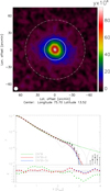 |
Fig. 1. Top panel: MILCA tSZ map of A2319. The solid and dashed white circles show the typical radius of the cluster, R500, and the shock radius, RSh, detected in the azimuthal profile. The beam FWHM is given by the white circle in the bottom left corner, and the black contours provide the S/N in units of 2σ. The gray thin lines present the profiles for each quadrant of A2319. Bottom panel: tSZ azimuthal profile of A2319. The black samples show the measured tSZ signal in the MILCA map, while the green, red, and blue solid lines plot the GNFW, GNFW+δ (extra outer slope), and GNFW+Sh (shock) best-fit models, respectively. The vertical dashed gray line corresponds to Rsh = (2.93 ± 0.05) R500. The residual, normalized by the error bars, χ, is also shown for all the models. |
![Mathematical equation: $$ \begin{aligned} P(x) = \left\{ \begin{array}{ll} \frac{P_0 P_{500}}{(c_{500}x)^\gamma \left[ 1 + (c_{500}x)^\alpha \right]^{(\beta -\gamma )/\alpha }}&x < x_{\rm Sh} \\ \frac{P_0 P_{500}}{(c_{500}x_{\rm Sh})^\gamma \left[ 1 + (c_{500}x_{\rm Sh})^\alpha \right]^{(\beta -\gamma )/\alpha }}\left(\frac{x}{x_{\rm Sh}}\right)^{-\delta }&x > x_{\rm Sh} \end{array}\!. \right. \end{aligned} $$](/articles/aa/full_html/2019/02/aa32468-17/aa32468-17-eq4.gif) (4)
(4)
Then, we used a GNFW model to which we added a jump in the pressure at radius xSh. We parameterized the pressure drop with the parameter QSh. We refer to this model as GNFW+Sh:
![Mathematical equation: $$ \begin{aligned} P(x) = \left\{ \begin{array}{ll} \frac{P_0 P_{500}}{(c_{500}x)^\gamma \left[ 1 + (c_{500}x)^\alpha \right]^{(\beta -\gamma )/\alpha }}&x < x_{\rm Sh} \\ \frac{P_0 P_{500}}{(c_{500}x_{\rm Sh})^\gamma \left[ 1 + (c_{500}x_{\rm Sh})^\alpha \right]^{(\beta -\gamma )/\alpha }}Q_{\rm Sh}\left(\frac{x}{x_{\rm Sh}}\right)^{-\delta }&x > x_{\rm Sh} \end{array}\!. \right. \end{aligned} $$](/articles/aa/full_html/2019/02/aa32468-17/aa32468-17-eq5.gif) (5)
(5)
While discrepancies between the GNFW model and the data allow for the characterization of the significance of the pressure drop at large radii, a shock is indicted by high values for δ in model GNFW+δ. Model GNFW+Sh is physically motivated and allows us to describe the ICM properties when a shock is clearly identified. From these pressure profile models, we computed the expected tSZ signal in Planck data by projecting the pressure profile on the line of sight according to Eq. (1) and convolving the projected signal with a Gaussian beam corresponding to the Planck tSZ angular resolution.
3. Method
The core of our analysis consists of characterizing the drop in pressure, as seen through the tSZ effect, in the outskirt of A2319. First, we constructed a tSZ map of A2319 at 7′ FWHM angular resolution using MILCA (Hurier et al. 2013) and Planck data (Planck Collaboration I 2016). This map is derived from a pixel- and scale-dependent linear combination of Planck frequency channels from 100 to 857 GHz (see also Hurier et al. 2015, for more details). We verified that using the Planck public tSZ maps at a resolution of 10′ FWHM (MILCA & NILC, Planck Collaboration XXII 2016) provides consistent results. In the top panel of Fig. 1, we present the tSZ map of A2319. We observe a clear tSZ signal from A2319, with a central value y0 ≃ 10−4, which exceeds 45σ per beam at this resolution. We note that the angular resolution of the tSZ map (shown as a white circle in Fig. 1) is smaller thab the projected characteristic radius of A2319, R500 = 18.4′ (Piffaretti et al. 2011). In the following we use this value for R500.
Then, we computed an azimuthally averaged tSZ profile using concentric annuli with a 2′ binning (≃9 samples per R500, ≃3.5 samples per beam). We applied the same binning procedure to the pressure profile model in order to account for pixelization effects. By construction, the noise in the MILCA tSZ map at 7′ FWHM has a typical correlation length of 5′ FWHM. It is thus mandatory to account for the full covariance matrix of the tSZ profile. The scanning strategy makes the noise in Planck data inhomogeneous (Planck Collaboration I 2016). Thus, we estimated the covariance matrix, 𝒞P, of the tSZ profile using 1000 simulations of inhomogeneous correlated Gaussian noise (see Planck Collaboration Int. V 2013, for a description of the noise simulation procedure). We verified that the noise properties of the simulations were consistent with those of the noise observed in the background of the A2319 tSZ map. We present the extracted tSZ profile and the associated uncertainties, up to 4 × R500, in the bottom panel of Fig. 1. We observe a clear drop in tSZ signal around R ≃ 2.8 × R500. We checked that this drop is not dominated by any preferential direction (see profiles per quadrant on Fig. A.1, only the southeast profile has a significantly larger spatial extension) and is consistent in several independent profiles that were extracted from different slices in the map.
We adjust the models presented in Sect. 2 to the measured tSZ profile using a Markov chain Monte Carlo approach and assuming that the uncertainties follow Gaussian statistics, using
 (6)
(6)
where  is the measured tSZ profile and P is the tSZ profile derived from the models. The best-fitting parameters are listed in Table 1 for the three pressure profile models that we consider: a GNFW pressure profile (GNFW), a GNFW pressure profile with a change in slope at R = RSh (GNFW+δ), and a GNFW pressure profile with a pressure drop at R = RSh (GNFW+Sh). Our analysis focuses on the large-scale behavior of the pressure profile of A2319, and we therefore fixed the parameters α, γ, and c500 to the values derived in Ghirardini et al. (2018) because they are related to the inner structure of the cluster. We fit for the parameters β and P0 in the case of model GNFW, β, P0, RSh, and 1/δ in the case of model GNFW+δ, and β, P0, RSh, and QSh for model GNFW+Sh, for which we fixed δ = β. We verified that the shock parameters δ, RSh, and QSh are not correlated with the other GNFW parameters, see Fig. B.1. This justifies that we did not marginalize over these parameters.
Best-fitting pressure profile parameters considering, (i) a GNFW profile, (ii) a GNFW profile and an outer slope, and (iii) a GNFW profile and a shock.
Models GNFW+δ and GNFW+Sh describe the observed profile well at all scales with a reduced  of 1.2 and 1.1, respectively. Model GNFW fails to describe the data with a
  , and model GNFW+Sh is favored by 8.6σ1 compared to a model GNFW+δ with δ = 202. In Fig. 2 we present the posterior likelihood function on the fitted parameters for model GNFW+δ. The parameter of the outer slope is constrained to δ > 84 at a 99% confidence level. This indicates that the tSZ drop located at RSh is due to a discontinuity in the pressure, corresponding to a shock in the ICM. In contrast, the slope of the pressure profile at radius R ≲ RSh is constrained to β = 4.30 ± 0.03. Model GNFW+Sh shows that no significant pressure is detected beyond RSh, with QSh = −0.012 ± 0.045. We note that this result does not depend on the value for δ in the GNFW+Sh model.
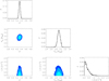 |
Fig. 2. Posterior likelihood functions for model GNFW+δ. Histograms on the diagonals present the marginalized likelihoods for parameters β, RSh, and 1/δ. The others panels show the marginalized likelihood, and the light blue, blue, and dark blue contours provide confidence levels at 68.3, 95.4, and 99.7%, respectively. |
4. Results and conclusion
The amplitude of the pressure discontinuity, QSh, is related to the Mach number of the infalling gas (Landau & Lifshitz 1959; Sarazin et al. 2002), ℳ, as
 (7)
(7)
where γg is the adiabatic index of the gas (we expect γg = 5/3 for a fully ionized plasma). In the case of A2319, no significant tSZ signal is observed at R > RSh, and only a lower limit can therefore be set on the Mach number. It is constrained to ℳ > 3.25 at a 95% confidence level. Following the results by Shi (2016), we can use the location of the virial shock to constrain the accretion rate of the galaxy cluster. Assuming γg = 5/3 and self-similarity, we obtain s = 1.36 ± 0.20, which corresponds to the cluster mass evolving as M(R)∝t3s/2.
Finally, we compared the virial shock radius to the galaxy number density profile of A2319, which we extracted using the 2MASS (Skrutskie et al. 2006) galaxy survey (see the top panel of Fig. 3). The galaxy number density profile is well described by a Navarro–Frenk–White (NFW) profile (Navarro et al. 1995) below 2.8 × R500, with a concentration cg = 1.00 ± 0.37. At radii R > 3 × R500, we observe a > 4σ deficit in the galaxy number density profile compared to an NFW profile extrapolation. Assuming that this drop corresponds to the splashback radius, Rsp = (3.2 ± 0.1)R500, we used the results from Shi (2016) to constrain the adiabatic index of the gas, in combination with the location of the virial shock. We present the corresponding posterior likelihood in the plane s–γg in the bottom panel of Fig. 3 and constrain the parameters to s = 1.29 ± 0.24 and γg = 1.65 ± 0.02. This result is consistent with the expectation of γg = 5/3, and it allows us to measure the accretion rate of A2319, Ṁ ≃ (1.4 ± 0.4) × 1014 M⊙ Gyr−1, in agreement with expectations from numerical simulation that considered the mass of A2319 (see, e.g., De Boni et al. 2016). This result illustrates that large-scale tSZ observations with high signal-to-noise ratio (S/N) can constrain galaxy cluster formation by directly probing the outskirts of galaxy clusters where the baryons are heated.
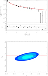 |
Fig. 3. Top panel: galaxy density profile of A2319 derived from the 2MASS catalog. The black samples show the data, and the solid red line shows the best-fitting NFW profile for R < 2.5 × R500. Bottom panel: accretion rate and equation-of-state likelihood. |
Estimated by computing the likelihood ratio.
δ = 20 is a threshold we chose to consider that the profile has no smooth change in slope. This value correspond to a drop in pressure by a factor of 2 over a distance of 0.1 R500.
Acknowledgments
We thanks R. Angulo, C. Hernández-Monteagudo, and O. Hahn for useful discussions. G.H. and R.A, acknowledge support from Spanish Ministerio de Economía and Competitividad (MINECO) through grant number AYA2015-66211-C2-2. U.K. acknowledges support by the Israel Science Foundation (ISF grant No. 1769/15). We acknowledge the use of HEALPix (Górski et al. 2005).
References
- Adam, R., Comis, B., Macías-Pérez, J. F., et al. 2014, A&A, 569, A66 [NASA ADS] [CrossRef] [EDP Sciences] [Google Scholar]
- Adam, R., Hahn, O., Ruppin, F., et al. 2018, A&A, 614, A118 [NASA ADS] [CrossRef] [EDP Sciences] [Google Scholar]
- Arnaud, M., Pratt, G. W., Piffaretti, R., et al. 2010, A&A, 517, A92 [NASA ADS] [CrossRef] [EDP Sciences] [Google Scholar]
- Bell, A. R. 1978a, MNRAS, 182, 147 [NASA ADS] [CrossRef] [Google Scholar]
- Bell, A. R. 1978b, MNRAS, 182, 443 [NASA ADS] [CrossRef] [Google Scholar]
- Bennett, C. L., Larson, D., Weiland, J. L., et al. 2013, ApJS, 208, 20 [Google Scholar]
- Birkinshaw, M. 1999, Phys. Rep., 310, 97 [NASA ADS] [CrossRef] [Google Scholar]
- Bleem, L. E., Stalder, B., de Haan, T., et al. 2015, ApJS, 216, 27 [NASA ADS] [CrossRef] [Google Scholar]
- Carlstrom, J. E., Holder, G. P., & Reese, E. D. 2002, ARA&A, 40, 643 [NASA ADS] [CrossRef] [Google Scholar]
- De Boni, C., Serra, A. L., Diaferio, A., Giocoli, C., & Baldi, M. 2016, ApJ, 818, 188 [NASA ADS] [CrossRef] [Google Scholar]
- Fixsen, D. J. 2009, ApJ, 707, 916 [Google Scholar]
- Ghirardini, V., Ettori, S., Eckert, D., et al. 2018, A&A, 614, A7 [NASA ADS] [CrossRef] [EDP Sciences] [Google Scholar]
- Górski, K. M., Hivon, E., Banday, A. J., et al. 2005, ApJ, 622, 759 [NASA ADS] [CrossRef] [Google Scholar]
- Hasselfield, M., Hilton, M., Marriage, T. A., et al. 2013, J. Cosmol. Astropart. Phys., 7, 008 [NASA ADS] [CrossRef] [Google Scholar]
- Hurier, G. 2016, A&A, 596, A61 [NASA ADS] [CrossRef] [EDP Sciences] [Google Scholar]
- Hurier, G., Macías-Pérez, J. F., & Hildebrandt, S. 2013, A&A, 558, A118 [NASA ADS] [CrossRef] [EDP Sciences] [Google Scholar]
- Hurier, G., Aghanim, N., Douspis, M., & Pointecouteau, E. 2014, A&A, 561, A143 [NASA ADS] [CrossRef] [EDP Sciences] [Google Scholar]
- Hurier, G., Douspis, M., Aghanim, N., et al. 2015, A&A, 576, A90 [NASA ADS] [CrossRef] [EDP Sciences] [Google Scholar]
- Keshet, U., Kushnir, D., Loeb, A., & Waxman, E. 2017, ApJ, 845, 24 [NASA ADS] [CrossRef] [Google Scholar]
- Keshet, U., & Reiss, I. 2017, ArXiv e-prints [arXiv:1709.07442] [Google Scholar]
- Keshet, U., Waxman, E., Loeb, A., Springel, V., & Hernquist, L. 2003, ApJ, 585, 128 [NASA ADS] [CrossRef] [Google Scholar]
- Kitayama, T., Ueda, S., Takakuwa, S., et al. 2016, PASJ, 68, 88 [NASA ADS] [CrossRef] [Google Scholar]
- Kocsis, B., Haiman, Z., & Frei, Z. 2005, ApJ, 623, 632 [NASA ADS] [CrossRef] [Google Scholar]
- Landau, L. D., & Lifshitz, E. M. 1959, Fluid mechanics (Oxford: Pergamon Press) [Google Scholar]
- Lau, E. T., Nagai, D., Avestruz, C., Nelson, K., & Vikhlinin, A. 2015, ApJ, 806, 68 [NASA ADS] [CrossRef] [Google Scholar]
- Loeb, A., & Waxman, E. 2000, Nature, 405, 156 [NASA ADS] [CrossRef] [Google Scholar]
- Miniati, F., Jones, T. W., Kang, H., & Ryu, D. 2001, ApJ, 562, 233 [NASA ADS] [CrossRef] [Google Scholar]
- Molnar, S. M., Hearn, N., Haiman, Z., et al. 2009, ApJ, 696, 1640 [Google Scholar]
- Nagai, D., Kravtsov, A. V., & Vikhlinin, A. 2007, ApJ, 668, 1 [NASA ADS] [CrossRef] [Google Scholar]
- Navarro, J. F., Frenk, C. S., & White, S. D. M. 1995, MNRAS, 275, 720 [NASA ADS] [CrossRef] [Google Scholar]
- O’Hara, T. B., Mohr, J. J., & Guerrero, M. A. 2004, ApJ, 604, 604 [NASA ADS] [CrossRef] [Google Scholar]
- Perrott, Y. C., Olamaie, M., Rumsey, C., et al. 2015, A&A, 580, A95 [NASA ADS] [CrossRef] [EDP Sciences] [Google Scholar]
- Piffaretti, R., Arnaud, M., Pratt, G. W., Pointecouteau, E., & Melin, J.-B. 2011, A&A, 534, A109 [NASA ADS] [CrossRef] [EDP Sciences] [Google Scholar]
- Planck Collaboration I. 2016, A&A, 594, A1 [NASA ADS] [CrossRef] [EDP Sciences] [Google Scholar]
- Planck Collaboration IV. 2016, A&A, 594, A4 [NASA ADS] [CrossRef] [EDP Sciences] [Google Scholar]
- Planck Collaboration XXII. 2016, A&A, 594, A22 [NASA ADS] [CrossRef] [EDP Sciences] [Google Scholar]
- Planck Collaboration Int. V. 2013, A&A, 550, A131 [NASA ADS] [CrossRef] [EDP Sciences] [Google Scholar]
- Planck Collaboration Int. X. 2013, A&A, 554, A140 [NASA ADS] [CrossRef] [EDP Sciences] [Google Scholar]
- Reiss, I., & Keshet, U. 2017, J. Cosmol. Astropart. Phys., 10, 10 [NASA ADS] [CrossRef] [Google Scholar]
- Sarazin, C. L. 1999, ApJ, 520, 529 [NASA ADS] [CrossRef] [Google Scholar]
- Sarazin, C. L. 2002, in Merging Processes in Galaxy Clusters, eds. L. Feretti, I. M. Gioia, & G. Giovannini, Astrophys. Space Sci. Lib., 272, 1 [NASA ADS] [Google Scholar]
- Shi, X. 2016, MNRAS, 461, 1804 [NASA ADS] [CrossRef] [Google Scholar]
- Skrutskie, M. F., Cutri, R. M., Stiening, R., et al. 2006, AJ, 131, 1163 [NASA ADS] [CrossRef] [Google Scholar]
- Sunyaev, R. A., & Zeldovich, Y. B. 1972, Comments Astrophys. Space Phys., 4, 173 [NASA ADS] [EDP Sciences] [Google Scholar]
- Totani, T., & Kitayama, T. 2000, ApJ, 545, 572 [NASA ADS] [CrossRef] [Google Scholar]
Appendix A: Profiles in the four quadrants
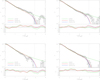 |
Fig. A.1. tSZ azimuthal profile of A2319. The black samples show the measured tSZ signal in the MILCA map, and the green, red, and blue solid lines plot the GNFW, GNFW+δ (extra outer slope), and GNFW+Sh (shock) best-fit models for the full azimuthal profile, respectively. The vertical dashed gray line corresponds to Rsh = (2.93 ± 0.05) R500. The residual, normalized by the error bars, χ, is also shown for all the models. From left to right and top to bottom, we present the profiles in the four quadrants: northeast, southeast, southwest, and northwest. |
Appendix B: Likelihood for all GNFW parameters
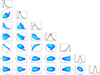 |
Fig. B.1. Likelihood function for the 3D pressure profile of A2319 for all parameters (P0, c500, α, β, γ, Rsh, and Qsh). Blue contours represent the 68%, 95%, and 99% confidence levels, and the red stars indicate the best-fit values. No significant correlations are observed between the shock parameters and the GNFW sector of the model. |
All Tables
Best-fitting pressure profile parameters considering, (i) a GNFW profile, (ii) a GNFW profile and an outer slope, and (iii) a GNFW profile and a shock.
All Figures
|
Fig. 1. Top panel: MILCA tSZ map of A2319. The solid and dashed white circles show the typical radius of the cluster, R500, and the shock radius, RSh, detected in the azimuthal profile. The beam FWHM is given by the white circle in the bottom left corner, and the black contours provide the S/N in units of 2σ. The gray thin lines present the profiles for each quadrant of A2319. Bottom panel: tSZ azimuthal profile of A2319. The black samples show the measured tSZ signal in the MILCA map, while the green, red, and blue solid lines plot the GNFW, GNFW+δ (extra outer slope), and GNFW+Sh (shock) best-fit models, respectively. The vertical dashed gray line corresponds to Rsh = (2.93 ± 0.05) R500. The residual, normalized by the error bars, χ, is also shown for all the models. |
| In the text | |
|
Fig. 2. Posterior likelihood functions for model GNFW+δ. Histograms on the diagonals present the marginalized likelihoods for parameters β, RSh, and 1/δ. The others panels show the marginalized likelihood, and the light blue, blue, and dark blue contours provide confidence levels at 68.3, 95.4, and 99.7%, respectively. |
| In the text | |
|
Fig. 3. Top panel: galaxy density profile of A2319 derived from the 2MASS catalog. The black samples show the data, and the solid red line shows the best-fitting NFW profile for R < 2.5 × R500. Bottom panel: accretion rate and equation-of-state likelihood. |
| In the text | |
|
Fig. A.1. tSZ azimuthal profile of A2319. The black samples show the measured tSZ signal in the MILCA map, and the green, red, and blue solid lines plot the GNFW, GNFW+δ (extra outer slope), and GNFW+Sh (shock) best-fit models for the full azimuthal profile, respectively. The vertical dashed gray line corresponds to Rsh = (2.93 ± 0.05) R500. The residual, normalized by the error bars, χ, is also shown for all the models. From left to right and top to bottom, we present the profiles in the four quadrants: northeast, southeast, southwest, and northwest. |
| In the text | |
|
Fig. B.1. Likelihood function for the 3D pressure profile of A2319 for all parameters (P0, c500, α, β, γ, Rsh, and Qsh). Blue contours represent the 68%, 95%, and 99% confidence levels, and the red stars indicate the best-fit values. No significant correlations are observed between the shock parameters and the GNFW sector of the model. |
| In the text | |
Current usage metrics show cumulative count of Article Views (full-text article views including HTML views, PDF and ePub downloads, according to the available data) and Abstracts Views on Vision4Press platform.
Data correspond to usage on the plateform after 2015. The current usage metrics is available 48-96 hours after online publication and is updated daily on week days.
Initial download of the metrics may take a while.