| Issue |
A&A
Volume 621, January 2019
|
|
|---|---|---|
| Article Number | A39 | |
| Number of page(s) | 13 | |
| Section | Cosmology (including clusters of galaxies) | |
| DOI | https://doi.org/10.1051/0004-6361/201833323 | |
| Published online | 03 January 2019 | |
Hydrostatic mass profiles in X-COP galaxy clusters
1
INAF, Osservatorio di Astrofisica e Scienza dello Spazio, Via Pietro Gobetti 93/3, 40129
Bologna, Italy
e-mail: This email address is being protected from spambots. You need JavaScript enabled to view it.
2
INFN, Sezione di Bologna, Viale Berti Pichat 6/2, 40127
Bologna, Italy
3
Dipartimento di Fisica e Astronomia Università di Bologna, Via Pietro Gobetti 93/2, 40129
Bologna, Italy
4
MPE, Giessenbachstrasse 1, 85748
Garching bei München, Germany
5
IRAP, Université de Toulouse, CNRS, CNES, UPS, 9 av. du colonel Roche, BP44346, 31028
Toulouse Cedex 4, France
6
INAF, IASF, Via E. Bassini 15, 20133
Milano, Italy
7
Department of Astrophysical Sciences, Princeton University, 4 Ivy Lane, Princeton, NJ, 08544-1001
USA
Received:
30
April
2018
Accepted:
4
October
2018
Abstract
Aims. We present the reconstruction of hydrostatic mass profiles in 13 X-ray luminous galaxy clusters that have been mapped in their X-ray and Sunyaev–Zeldovich (SZ) signals out to R200 for the XMM-Newton Cluster Outskirts Project (X-COP).
Methods. Using profiles of the gas temperature, density, and pressure that have been spatially resolved out to median values of 0.9R500, 1.8R500, and 2.3R500, respectively, we are able to recover the hydrostatic gravitating mass profile with several methods and using different mass models.
Results. The hydrostatic masses are recovered with a relative (statistical) median error of 3% at R500 and 6% at R200. By using several different methods to solve the equation of the hydrostatic equilibrium, we evaluate some of the systematic uncertainties to be of the order of 5% at both R500 and R200. A Navarro-Frenk-White profile provides the best-fit in 9 cases out of 13; the remaining 4 cases do not show a statistically significant tension with it. The distribution of the mass concentration follows the correlations with the total mass predicted from numerical simulations with a scatter of 0.18 dex, with an intrinsic scatter on the hydrostatic masses of 0.15 dex. We compare them with the estimates of the total gravitational mass obtained through X-ray scaling relations applied to YX, gas fraction, and YSZ, and from weak lensing and galaxy dynamics techniques, and measure a substantial agreement with the results from scaling laws, from WL at both R500 and R200 (with differences below 15%), from cluster velocity dispersions. Instead, we find a significant tension with the caustic masses that tend to underestimate the hydrostatic masses by 40% at R200. We also compare these measurements with predictions from alternative models to the cold dark matter, like the emergent gravity and MOND scenarios, confirming that the latter underestimates hydrostatic masses by 40% at R1000, with a decreasing tension as the radius increases, and reaches ∼15% at R200, whereas the former reproduces M500 within 10%, but overestimates M200 by about 20%.
Conclusions. The unprecedented accuracy of these hydrostatic mass profiles out to R200 allows us to assess the level of systematic errors in the hydrostatic mass reconstruction method, to evaluate the intrinsic scatter in the NFW c − M relation, and to robustly quantify differences among different mass models, different mass proxies, and different gravity scenarios.
Key words: dark matter / X-rays: galaxies: clusters / galaxies: clusters: intracluster medium
Einstein and Spitzer Fellow.
© ESO 2019
1. Introduction
The use of the galaxy clusters as astrophysical laboratories and cosmological probes relies on characterizing the distribution of their gravitational mass (see e.g. Allen et al. 2011; Kravtsov & Borgani 2012). In the currently favoured Λ cold dark matter (CDM) scenario, clusters of galaxies are dominated by dark matter (80% of the total mass), with a negligible contribution due to stars (a small percentage; see e.g. Gonzalez et al. 2013), and even less by cold/warm gas, and the rest (about 15% of the total mass, i.e. MDM/Mgas∼ 4–7) in the form of ionized plasma emitting in X-ray and detectable through the Sunyaev–Zeldovich (SZ, Sunyaev & Zeldovich 1972) effect induced from inverse Compton scattering of the cosmic microwave background photons off the electrons in the hot intracluster medium (ICM).
X-ray observations can provide an estimate of the total mass in galaxy clusters under the condition that the ICM is in hydrostatic equilibrium within the gravitational potential. This is an assumption that is satisfied if the ICM, treated as collisional fluid on timescales typical of any heating/cooling/dynamical process much longer than the elastic collisions time for ions and electrons, is crossed by a sound wave on a timescale shorter than the cluster’s age (e.g. Ettori et al. 2013a), as generally occurs in clusters that are not undergoing any major merger and can be considered relaxed from a dynamical point of view.
Given this condition, the ability to resolve the mass distribution in X-rays depends on the ability to make spatially resolved measurements of the gas temperature and density. This ability is limited severely by many systematic effects, such as the presence of gas inhomogeneities on small and large scales that can bias the measurements of the gas density (e.g. Roncarelli et al. 2013), contamination from the X-ray background that reduce the signal-to-noise ratio and the corresponding robustness of the spectral measurements (e.g. Ettori & Molendi 2011; Reiprich et al. 2013); adopted assumptions, for example on the halo geometry (see e.g. Buote & Humphrey 2012; Sereno et al. 2017a) and the dynamical state (see e.g. Nelson et al. 2014a; Biffi et al. 2016) of the objects, where mergers are the major source of violation of the hydrostatic equilibrium assumption (e.g. Khatri & Gaspari 2016); and inhomogeneities in the temperature distribution, which also play a role (Rasia et al. 2012). Within 0.15 R500, turbulence driven by the active galactic nucleus feedback (e.g. Gaspari et al. 2018) is instead responsible for the major deviations.
In recent years, the great improvement in instrumentation in detecting and characterizing the SZ signal has also allowed us to use this piece of information to resolve the pressure profile of the intracluster plasma. Our XMM-Newton Cluster Outskirts Project (X-COP; Eckert et al. 2017) has now completed the joint analysis of XMM-Newton and Planck exposures of 13 nearby massive galaxy clusters, permitting us to resolve X-ray and SZ signals out to the virial radius (∼R200), also correcting for gas clumpiness as resolved with the XMM point spread function of about 15 arcsec (∼17 kpc at the mean redshift of our sample of 0.06). In this paper, which appears as a companion to the extended analysis of the X-COP sample presented in Ghirardini et al. (2019, on the thermodynamical properties of the sample) and Eckert et al. (2019, on the non-thermal pressure support), we report on the reconstruction of the hydrostatic mass in these systems and how it compares with several independent estimates.
The paper is organized as follows. In Sect. 2 we present the observed profiles of the thermodyncamical properties. We describe in Sect. 3 the different techniques adopted to recover the hydrostatic masses. In Sect. 4 we compare these dark matter profiles with those recovered from scaling laws, weak lensing, and galaxy dynamics. A comparison with predictions from the modified Newtonian dynamics and the emergent gravity scenario is discussed in Sect. 5. We summarize our main findings in Sect. 6. Unless mentioned otherwise, the quoted errors are statistical uncertainties at the 1σ confidence level.
In this study, we often refer to radii, RΔ, and masses, MΔ, which are the corresponding values estimated at the given overdensity Δ as  , where
  is the critical density of the universe at the observed redshift z of the cluster, and Hz = H0 [ΩΛ+Ωm(1+z)3]0.5 = H0 hz is the value of the Hubble constant at the same redshift. For the ΛCDM model, we adopt the cosmological parameters H0 = 70 km s−1 Mpc−1 and Ωm = 1 − ΩΛ = 0.3.
2. The X-COP sample
The XMM-Newton Cluster Outskirts Project (X-COP, Eckert et al. 2017) is an XMM Very Large Program (PI: Eckert) dedicated to the study of the X-ray emission in cluster outskirts. It targets 12 local, massive galaxy clusters selected for their high signal-to-noise ratios in the Planck all-sky SZ survey (S/N > 12 in the PSZ1 sample, Planck Collaboration XXIX 2014) as resolved sources (R500> 10 arcmin) in the redshift range 0.04 < z < 0.1 and along the directions with a galactic absorption lower than 1021 cm−2 to avoid any significant suppression of the X-ray emission in the soft band where most of the spatial analysis is performed. These selection criteria guarantee that a joint analysis of the X-ray and SZ signals allows the reconstruction of the ICM properties out to R200 for all our targets. A complete description of the reduction and analysis of our proprietary X-ray data and of the SZ data for X-COP is provided in Ghirardini et al. (2019; see also Eckert et al. 2019). We note here that our new Planck pressure profiles are extracted using exactly the same method as in Planck Collaboration Int. V (2013), but on the Planck 2015 data release (i.e. the full intensity survey) which has a higher S/N (due to the higher exposure time) and improved data processing and calibration. To the original X-COP list of 12 clusters, we added HydraA (Abell 780) due to the availability of a high-quality XMM-Newton mapping (De Grandi et al. 2016). The X-ray signal extends out to R200 and therefore it is possible to recover its hydrostatic mass with very high precision, even though the Planck signal for this cluster is contaminated by a bright central radio source.
Here, we summarize the properties of the quantities of interest for the reconstruction of the gravitating mass distribution. The physical quantities directly observable are the density ngas and temperature Tgas of the X-ray emitting gas, and the SZ pressure Pgas of the same plasma. Their radial profiles are presented in Fig. 1. The gas density is obtained from the geometrical deprojection of the X-ray surface brightness out to a mean value of 1.8R500. Thanks to the observational strategy implemented in X-COP, we are able to correct the X-ray emission for the presence of gas clumps both by masking substructures spatially resolved with XMM-Newton and by measuring the azimuthal median, instead of the azimuthal mean (Zhuravleva et al. 2013; Eckert et al. 2015). The estimates of the gas temperature are based on the modelling with an absorbed thermal component of the XMM-Newton spectra extracted from concentric annuli around the X-ray peak in the [0.5–12] keV energy band and corrected from the local sky background components. A typical statistical error lower than 5% is associated with these spectral measurements. On average, the temperature profiles are resolved out to 0.9R500. The SZ electron pressure profile is obtained following the method described in Planck Collaboration Int. V (2013) from the Planck PSF deconvolution and geometrical deprojection of the azimuthally averaged integrated Comptonization parameter y extracted from a re-analysis of the SZ signal mapped with Planck and that extends up to ∼2.3R500.
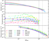 |
Fig. 1. From top to bottom panels: reconstructed electron density, projected temperature, and SZ pressure profiles as functions of the radius in scale units of R500. Statistical error bars are overplotted. The two vertical lines indicate R500 and R200. |
3. Total gravitating mass from the hydrostatic equilibrium equation
Under the assumption that the ICM has a spherically symmetric distribution and follows the equation of state for a perfect gas, Pgas = kTgasngas, where k is the Boltzmann constant, the combination of the gas density ngas, as the sum of the electron and proton densities ne + np ≈ 1.83ne, with the X-ray spectral measurements of the gas temperature and/or the SZ derived gas pressure, allows us to evaluate the total mass within a radius r through the hydrostatic equilibrium equation (see e.g. Ettori et al. 2013a)
 (1)
(1)
where G is the gravitational constant, mu = 1.66 × 10⁻²⁴ g is the atomic mass unit, and μ = ρgas/(mungas) ≈ (2X + 0.75Y + 0.56Z)−1 ≈ 0.6 is the mean molecular weight in atomic mass unit for ionized plasma, with X, Y, and Z being the mass fraction for hydrogen, helium, and other elements, respectively (X + Y + Z = 1, with X ≈ 0.716 and Y ≈ 0.278 for a typical metallicity of 0.3 times the solar abundance from Anders & Grevesse 1989).
In the present analysis, we apply both the backward and the forward method (see e.g. Ettori et al. 2013a), as discussed and illustrated in our pilot study on A2319 (Ghirardini et al. 2018). We use all the information available (measured pressure Pm, temperature Tm, and emissivity ϵm) to build a joint likelihood ℒ,
![Mathematical equation: $$ \begin{aligned} \begin{aligned} \log \mathcal{L} =&-0.5 \left[ (P-P_{\rm {m}}) \Sigma _{\mathrm{tot}}^{-1} (P-P_{\rm {m}})^T + n \log \left( \det \left( \Sigma _{\mathrm{tot}} \right) \right) \right] \\&-0.5 \sum _{i=1}^{n_{T}} \left[ \frac{(T_i-T_{\mathrm{m},i})^2}{\sigma _{T,i}^2+\sigma _{T,\mathrm{int}}^2} + \log \left( {\sigma _{T,i}^2+\sigma _{T,\mathrm{int}}^2} \right) \right] \\&-0.5 \left[ \sum _{j=1}^{n_{\epsilon }} \frac{(\epsilon -\epsilon _{\mathrm{m},j})^2}{\sigma _{\epsilon ,j}^2} \right], \end{aligned} \end{aligned} $$](/articles/aa/full_html/2019/01/aa33323-18/aa33323-18-eq4.gif) (2)
(2)
that combines in the fitting procedure (i) the χ2 related to the measured profiles [i.e.  ,
,  , and
, and  ; see Table A.2], (ii) an intrinsic scatter σT, int to account for any tension between X-ray and SZ measurements, and (iii) the covariance matrix Σtot among the data in the Planck pressure profile (for details, see Appendix D in Ghirardini et al. 2018).
The emissivity ϵ is obtained from the multiscale fitting (Eckert et al. 2016, see also Sect. 2.3 in Ghirardini et al. 2019) of the observed X-ray surface brightness. In the backward method, a parametric mass model is assumed and combined with the gas density profile to predict a gas temperature profile T that is then compared with the one measured Tm in the spectral analysis and the one estimated from SZ as P/ngas (losing the spatial resolution in the inner regions because of the modest 7 arcmin FWHM angular resolution of our Planck SZ maps, but gaining in radial extension due to the Planck spatial coverage; Planck Collaboration Int. V 2013) to constrain the mass model parameters. In the forward method, some functional forms are fitted to the deprojected gas temperature and pressure profiles, as detailed in Ghirardini et al. (2018), with instead no assumptions on the form of the gravitational potential. We note that we neglect the three innermost Planck points for the analysis to avoid possible biases induced by the Planck beam. The hydrostatic equilibrium equation (Eq. (1)) is then directly applied to evaluate the radial distribution of the mass.
The profiles are fitted using an MCMC approach based on the code emcee (Foreman-Mackey et al. 2013) with 10 000 steps and about 100 walkers, and throwing away the first 5000 points because of “burnt-in” time. From the resulting posterior distribution on our parameters, we estimate the reference values using the median of the distributions, and the errors as half the difference between the 84th and 16th percentiles. The best-fit parameters In the present analysis, we investigate different mass models (Sect. 3.1), and adopt as reference model a NFW mass model with two free parameters, the mass concentration and R200 (see Sect. 3.2).
3.1. Comparison among different mass models with the backward method
We apply the backward method with the following set of different mass models and estimate their maximum likelihood in reproducing the observed profiles of gas density, temperature and SZ pressure.
The mass profile is parametrized through the expression
 (3)
(3)
where Δ = 200, hz = Hz/H0, and x = r/rs, with the scale radius rs and the concentration c being the two free parameters of the fit. The function F(x) characterizes each mass model and is defined as follows:
NFW: F(x)=log(1 + x)−x/(1 + x) (Navarro et al. 1997);
EIN:
F(x)=a1 − a1/2a1ea0γ(a1, a0x1/a) with a = 5, a0 = 2n, a1 = 3n, and γ(a, y) being the incomplete gamma function equal to  (from Eq. (A2) in Mamon & ᴌokas 2005);
ISO:
 , which is the King approximation to the isothermal sphere (King 1962);
BUR: F(x)=log(1 + x2)+2log(1 + x)−2arctan(x) (Salucci & Burkert 2000);
HER:
 (Hernquist 1990).
We note that our observed profiles cannot provide any robust constraint on the third parameter a of the Einasto profile that is therefore fixed to a value of 5 as observed for massive halos (e.g. Dutton & Macciò 2014). Moreover, the parameter c is defined as the “concentration” in the NFW profile, whereas it represents a way to constrain the normalization for the other mass models. In our MCMC approach, we adopt for c a uniform a-prior distribution in the linear space in the range 0.1–15. The a-prior distributions on the scale radius (or R200 = c × rs for the NFW case) are still defined as uniform in the linear space in the following ranges: 1–3 Mpc (NFW); 0.1–2.8 Mpc (EIN); 0.02–0.8 Mpc (ISO); 0.02–0.8 Mpc (BUR); 0.2–3 Mpc (HER).
We show all the mass profiles in Fig. A.1. In Table A.1, we quote all the best-fit parameters, and the relative Bayesian Evidence E estimated, for each mass model, as the integral of the likelihood function ℒ (Eq. (2)) over the a-prior distributions P(θ) of the parameters θ (E = ∫ℒ(θ)P(θ)dθ; as implemented in e.g. MultiNest, Feroz et al. 2009).
In Fig. 2, we present the Bayes factor estimated for each object as the difference between the logarithm of the Bayesian evidence of the mass model with the highest evidence with respect to the others. Nine out of 13 objects prefer a NFW model fit and have data that are significantly inconsistent (Bayes factor > 5) with an isothermal/Burkert mass model. The remaining four objects prefer different mass models (ISO for A2255 and A2319, HER for A1644, and BUR for A644), but do not show any statistically significant (Bayes factor < 5) tension with NFW. Of those four objects, two (A2255 and A2319) are the ones with the highest value of the central entropy among the X-COP sample as estimated in Cavagnolo et al. (2009), strongly suggesting that they are disturbed systems that have produced a core (well modelled by an ISO profile) in the gravitational potential as a consequence of the ongoing merger. The case of A2319 has been indeed extensively studied in Ghirardini et al. (2018). A2255 shows a flat surface-brightness profile in its core and an X-ray morphology extended along the E-W axis (Sakelliou & Ponman 2006). Interestingly, the X-ray centroid of the cluster does not coincide with a dominant galaxy (Burns et al. 1995), which more strongly supports the merger scenario. The cluster also exhibits an unusual polarized radio halo which may be a radio relic seen in projection (Pizzo & de Bruyn 2009). A644 is an unusual radio-quiet cool-core cluster with a temperature profile rising inward and the cD galaxy positioned approximately between the X-ray peak and centroid, as expected for a merger origin of the properties of the X-ray emission in the core (Buote et al. 2005). We also note that it shows a steep gradient in the outermost points of the spectral temperature profile, which also suggests that the object can be dynamically non-relaxed in the regions at r > 0.4R500. We do not find any peculiarity in the observed profiles of A1644, confirming that, as also probed in the numerical simulations, a NFW profile provides a good description of the spherically averaged equilibrium density profiles of CDM halos; however, deviations are expected.
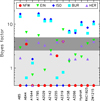 |
Fig. 2. Bayes factor of the mass models investigated with respect to the one with the highest evidence (see Table A.1). Shaded regions identify values of the Bayes factor where the tension between the models is either weak (< 2.5) or strong (> 5) according to the Jeffreys scale (Jeffreys 1961). |
3.2. Reference mass model: backward method with NFW mass model
We present the results of our analysis with a backward method and a NFW mass model in Table 1. We measure mean relative errors (statistical only) lower than 8% (median, mean, and dispersion at Δ = 1000, 500, and 200, respectively: 3, 4, 2%; 4, 5, 2%; 6, 7, 3%; see Fig. 3).
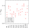 |
Fig. 3. Relative error (at 1σ) on the hydrostatic mass recovered with the backward method and a NFW model (see Table 1). |
Values of the total gravitating mass as estimated with the backward method and a NFW model at some radii of reference (0.5, 1, 1.5 Mpc) and at the overdensities of 500 and 200 with respect to the critical density of the universe at the cluster’s redshift.
In the cold dark matter scenario, the structure formation is hierarchical and allows the build-up of the most massive gravitationally bound halos, like galaxy clusters, only at later cosmic times. Considering that the central density of halos reflects the mean density of the Universe at the time of formation, halos with increasing mass are expected to have lower mass concentration at given redshift (e.g. Navarro et al. 1997; Bullock et al. 2001; Dolag et al. 2004; Diemer & Kravtsov 2015).
We can investigate how our best-fit results on NFW concentration and M200 (quoted in Table 1) reproduce the predictions from numerical simulations. We can also assess the level of the intrinsic scatter in the c200 − M200 relation in this mass range. Simulations suggest that this scatter is related to the variation in formation time and is expected to be lower in more massive halos that formed more recently (e.g. Neto et al. 2007).
We model the relation with a standard power law:
 (4)
(4)
The intrinsic scatter σc|M of the concentration around a given mass, c200(M200), is taken to be lognormal (Duffy et al. 2008; Bhattacharya et al. 2013).
We fit the data with a linear relation in decimal logarithmic (log) variables with the R-package LIRA1. LIRA is based on a Bayesian hierarchical analysis which can deal with heteroscedastic and correlated measurements uncertainties, intrinsic scatter, scattered mass proxies, and time-evolving mass distributions (Sereno 2016).
The mass distribution of the fitted clusters has to be properly modelled to address Malmquist and Eddington biases (Kelly 2007). The Gaussian distribution can provide an adequate modelling (Sereno & Ettori 2015b). The parameters of the distribution are found within the regression procedure. This scheme is fully effective in modelling both selection effects at low masses and the steepness of the cosmological halo mass function at large masses.
Performing an unbiased analysis of the concentration–mass (c-M) relation requires properly addressing the uncertainties connected to the correlations and intrinsic scatter. Measured mass and concentration are indeed strongly anti-correlated, causing the c-M relation to appear steeper (Auger et al. 2013; Dutton & Macciò 2014; Du & Fan 2014; Sereno et al. 2015). By correcting for this effect, it is possible to obtain a more precise, significantly flatter relation (Sereno et al. 2015). On the other hand, the intrinsic scatter of the measurable mass with respect to the true mass can bias the estimated slope towards flatter values (Rasia et al. 2013; Sereno & Ettori 2015a). To correct for this effect, we measure the concentration–mass uncertainty covariance matrix for each cluster from the MCMC chains, whereas we model the intrinsic scatter as a free fit parameter to be found in the regression procedure.
Adopting non-informative priors (Sereno et al. 2017b) we find α = 0.89 ± 0.90 and β = −0.42 ± 0.98, in agreement with theoretical predictions for slope and normalization (see Fig. 4). Statistical uncertainties are very large and we cannot discriminate between the different theoretical predictions.
 |
Fig. 4. Left panel: concentration–mass relation of the X-COP clusters. The dashed black lines show the median scaling relation (full black line) plus or minus the intrinsic scatter at redshift z = 0.06. The shaded grey region encloses the 68.3% confidence region around the median relation due to uncertainties on the scaling parameters. As reference, we plot the concentration–mass relations of Bhattacharya et al. (2013, blue line), Dutton & Macciò (2014, green line), Ludlow et al. (2016, orange line), and Meneghetti et al. (2014, solid and dashed red lines). The dashed red lines enclose the 1-σ scatter region in the theoretical concentration–mass relation from the MUSIC-2 N-body/hydrodynamical simulations. Empty circles identify the four objects (A644, A1644, A2255, A2319; see Fig. 2) for which NFW does not represent the best-fit mass model. Right panel: probability distributions of the parameters of the concentration–mass relation. The thick and thin black contours include the 1-σ and 2-σ confidence regions in two dimensions, here defined as the regions within which the probability is larger than exp(−2.3/2) and exp(−6.17/2) of the maximum, respectively. The red disk represents the parameters found by Meneghetti et al. (2014) for the relaxed sample. The bottom row plots the marginalized 1D distributions, renormalized to the maximum probability. The thick and thin black levels denote the confidence limits in one dimension, i.e. exp(−1/2) and exp(−4/2) of the maximum. |
On the other hand, mass measurement uncertainties are very small and we can estimate the intrinsic scatter of the hydrostatic masses, σMHE|M = 0.15 ± 0.08. Even though the marginalized posterior distribution of σMHE|M is peaked at ∼0.15 (see Fig. 4), smaller values are fully consistent. The posterior probability that σMHE|M is less than 10% (i.e. σMHE|M < 0.043) is 15%. Our estimate of hydrostatic mass scatter is in agreement with results from higher-z samples (Sereno & Ettori 2015a) and larger, even though compatible within uncertainties, with results from numerical simulations (Rasia et al. 2012).
The intrinsic scatter of the c-M relation, σc|M = 0.18 ± 0.06, is compatible with theoretical predictions (Bhattacharya et al. 2013; Meneghetti et al. 2014, σc|M ∼ 0.15) and previous observational constraints (e.g. Ettori et al. 2010; Mantz et al. 2016). The relation between mass and concentration for subsamples can differ from the general relation due to selection effects. Intrinsically overconcentrated clusters may be over-represented in a sample of clusters selected according to their large Einstein radii or to the apparent X-ray morphology (Meneghetti et al. 2014; Sereno et al. 2015). Intrinsic scatter of the c-M relation for relaxed samples is expected to be smaller than for the full population of mass selected halos. However, given the statistical uncertainty on the measured σc|M, we cannot draw any firm conclusion on the equilibrium status of the clusters.
3.3. Comparison of different methods and systematic errors
To evaluate some of the systematic uncertainties affecting our measurements of the hydrostatic mass, we estimate the mass at some fixed physical radii (500, 1000, and 1500 kpc) and at two overdensities (R500 and R200) using the forward method and the other mass models described in Sect. 3.1, and compare them to the results obtained from our model of reference (backward NFW). We summarize the results of this comparison in Table 2.
We observe that the use of the forward method (with or without SZ profiles) introduces a small systematic error at any radius, with a median difference of about 4% at R500, and < 2% (1st-3rd quartile: −5.4 / +8.1%) at R200.
Any other mass model constrained with the backward method introduces some systematic uncertainties that depends mainly on the shape characteristic of the model and on the fact that all the models have only two parameters, implying that it is not flexibile enough to accommodate the distribution in the observed profiles. For instance, we note that cored profiles, like ISO and BUR, present larger positive (negative) deviations in the core (outskirts) up to about 25%.
We note that this budget of the systematic uncertainties does not include other sources of error, such as any non-thermal contribution to the total gas pressure (e.g. Nelson et al. 2014b; Sereno et al. 2017a), and terms that account for either departures from the hydrostatic equilibrium (e.g. Nelson et al. 2014a; Biffi et al. 2016) or the violation of the assumed sphericity of the gas distribution (e.g. Sereno et al. 2017a). All these contributions have been shown to affect the clusters’ outskirts more significantly and tend to bias the total mass estimates higher (by 10–30%) at r > R500, with smaller effects in the inner regions. In particular, by imposing the distribution of the cluster mass baryon fraction estimated in the state-of-art hydrodynamical cosmological simulations, we evaluate in Eckert et al. (2019) a median value of about 6% and 10% at R500 and R200, respectively, for the relative amount of non-thermal pressure support in the X-COP objects.
4. Comparison with mass estimates from scaling laws, weak lensing, and galaxy dynamics
We compare our estimates of the hydrostatic mass with constraints obtained from (i) X-ray based scaling relations applied to YX = Mgas × T (Vikhlinin et al. 2009), gas mass fraction (Mantz et al. 2010, also including a correction factor of 0.9 for Chandra calibration updates; see caption of their Table 4), and SZ signal (the Planck mass proxy MYz in Planck Collaboration XXIV 2016); (ii) weak lensing signals associated with the coherent distortion in the observed shape of background galaxies (as measured in the Multi Epoch Nearby Cluster Survey, MENeaCS; Herbonnet et al., in prep.); and (iii) galaxy dynamics either through the estimate of the velocity dispersion (Zhang et al. 2017) or via the caustic method (Rines et al. 2016; for A2029 we consider the recent measurement in Sohn et al. 2018), which calculates the mass from the escape velocity profile which is defined from the edges (i.e. the “caustics”) of the distribution in the redshift-projected radius diagram. The comparison is done by evaluating the hydrostatic MNFW at the radius defined by the other methods at a given overdensity (Δ = 500 for X-ray and SZ scaling laws, galaxy dynamics, and WL; Δ = 200 for WL and caustics). We plot the medians and the error-weighted means of the ratios M/MNFW in Fig. 5.
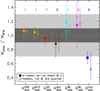 |
Fig. 5. Comparison between the backward NFW model and estimates of the mass from X-ray scaling relations (YX from Vikhlinin et al. 2009 – label on X-axis: |


Mass estimates based on X-ray scaling laws provide a very reassuring agreement: we measure a median ratio M/MNFW of 1.06 and 1.03 for the nine and six objects in common with Vikhlinin et al. (2009) and Mantz et al. (2010), respectively. For the 11 objects in common with Planck-SZ catalog (Hydra-A and Zw1215 are not included there), we measure a median (1st-3rd quartile) of 0.98 (0.92–1.01) and an error-weighted mean of 0.96 (rms 0.08)2.
A similarly good agreement is obtained with the six WL measurements in common: the medians are 1.16 (error-weighted mean 1.18 ± 0.12; rms 0.26) and 1.17 (error-weighted mean 1.14 ± 0.12; rms 0.32) at R500 and R200, respectively.
Considering the eight clusters in common with Zhang et al. (2017), we measure a median of 0.96, with 1st-3rd quartiles of 0.78–1.10. On the other hand, a clear tension is measured with respect to the six mass values obtained from caustics: MCau/MNFW has a median of 0.52 (1st-3rd quartiles: 0.39–0.75; error-weighted mean 0.68 ± 0.02; rms 0.08), with ratios smaller than 0.5 in three objects (A85: 0.43; A2142: 0.39; ZW1215: 0.35), and deviations larger than 3 σ, when statistical uncertainties on the single measurements are propagated, on three clusters (A1795: 11.5 σ; A2029: 6.5 σ; A2142: 3.9 σ). Simulations in Serra & Diaferio (2013), among others, show this might be the case when an insufficient number of spectroscopic member galaxies are adopted to constrain the caustic amplitude. We also note that caustic masses depend on a calibration constant that is function of the mass density, potential and galaxies’ velocity anisotropy profiles. This constant is generally calibrated with numerical simulations, and its value (between 0.5 and 0.7) has been debated in recent literature due to its dependence on the dynamical tracers adopted in the caustic technique (see e.g. Serra et al. 2011; Gifford et al. 2013, 2017). In the present analysis, we rely only on published results and postpone to further investigation, also on the role of this calibration constant, the study of the detected tension with estimates from caustic masses for the X-COP objects.
5. Comparison of predictions from the emergent gravity scenario and MOND
The lack of a valuable candidate particle for the cold dark matter has induced part of the community to search for alternative paradigms on how gravity works at galactic and larger scales. In galaxy clusters, the largest gravitationally bound structures in the universe, visible matter can account for only a fraction of the total gravitational mass. These systems thus represent a valid and robust test for models that try to explain this missing mass problem. Among these rivals of the current cosmological paradigm, we consider here two models, one that introduces modifications in the Newtonian dynamical laws (MOND, Milgrom 1983) and another that compensates for the required extra gravitational force by an emergent gravity (Verlinde 2017). They can both be described by similar equations, are able to describe the behaviour of the gravity on galactic scales, but are also known to cause trouble when applied on larger scales (called the “upscaling problem” in Massimi 2018), where for instance MOND predicts a gravitational acceleration that is too weak, suggesting that it can be an incomplete theory.
In the emergent gravity scenario, dark matter can appear as a manifestation of an additional gravitational force describing the “elastic” response due to the displacement of the entropy that can be associated with the thermal excitations carrying the positive dark energy, and with a strength that can be described in terms of the Hubble constant and of the baryonic mass distribution. For a spherically symmetric, static, and isolated astronomical system, Verlinde (2017) provides a relation between the emergent dark matter and the baryonic mass (see his Eq. (7.40)) that can be rearranged to isolate the dark matter component MDM. Following Ettori et al. (2017), we can write
 (5)
(5)
where  is the baryonic mass equal to the sum of the gas and stellar masses, and δB is equal to
  with
with  representing the mean baryon density within the spherical volume V(< r). In our case, the gas mass has been obtained from the integral over the cluster’s volume of the gas density (Fig. 1). The stellar mass has been estimated using a Navarro-Frenk-White (NFW, Navarro et al. 1997) profile with a concentration of 2.9 (see e.g. Lin et al. 2004) and by requiring the Mstar(< R500)/Mgas(< R500)=0.39 (M500/1014M⊙)−0.84 (Gonzalez et al. 2013). For the X-COP objects, we measure a median Mstar/Mgas of 0.09 (0.07–0.12 as 1st and 3rd quartile) at R500.
As we discuss in Ettori et al. (2017), Eq. (5) can be expressed as an acceleration gEG depending on the acceleration gB induced from the baryonic mass
 (6)
(6)
where y = 6/(cH0)×gB/(1 + 3δB).
Equation (6) takes a form very similar to the one implemented in MOND (e.g. Milgrom & Sanders 2016) with a characteristic acceleration a0 = cH0(1 + 3δB)/6. MOND is another theory that accounts for the mass in galaxies and galaxy clusters without a dark component and by modifying Newtonian dynamics, and requires an acceleration gMOND = gB (1+y−1/2), with y = gB/a0 and a0 = 10−8 cm s−2. For sake of completeness, we have also estimated a gravitating mass associated with a MOND acceleration.
The results of our comparison are shown in Fig. 6 (where we present as an example the case of A2142; the other mass profiles are shown in Fig. B.1). Although in the inner cluster regions the mismatch is indeed significant, with mass values from modified gravities that underestimate the hydrostatic quantities by a factor of few, over the radial interval between R1000 and R200, the medians of the distribution of the ratios between the mass estimates obtained from modified accelerations and from the hydrostatic equilibrium equation are in the range 0.6–0.87 for the MOND (consistent with previous studies; e.g. Pointecouteau & Silk 2005) and between 0.88 and 1.19 for EG, with the latter that indicates a nice consistency at R500 where MEG/MHyd ≈ 1.07 (0.99–1.12 as 1st and 3rd quartiles).
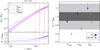 |
Fig. 6. Left panel: typical hydrostatic, EG and MOND radial mass profiles (here for A2142; plots for the remaining 12 objects in Appendix B. Vertical lines indicate R1000 (dotted line), R500 (dash-dotted line) and R200 (dashed line). Right panel: medians (and 1st and 3rd quartiles) of the ratio between the hydrostatic mass and the value predicted from EG and MOND for the whole X-COP sample. Shaded regions indicate the < 10% (darkest) and < 30% differences. |
6. Conclusions
We have investigated the hydrostatic mass profiles in the X-COP sample of 13 massive X-ray luminous galaxy clusters for which the gas density and temperature (from XMM-Newton X-ray data) and SZ pressure profiles (from Planck) are recovered at very high accuracy up to about R500 for the temperature and at R200 for density and pressure.
We constrain the total mass distribution by applying the hydrostatic equilibrium equation on these profiles, reconstructed under the assumption that the ICM follows a spherically symmetric distribution and using two different methods and five mass models. By adopting as reference model a NFW mass profile constrained with the backward method, we estimate the radial mass distribution up to R200 with a mean statistical relative error lower than 8%. A forward method, which is independent from any assumption on the shape of the gravitational potential, provides consistent results within 5% both at R500 and R200. Published results on the estimates of the hydrostatic mass in local massive galaxy clusters have so far reached statistical uncertainties larger than 10% (e.g. Pointecouteau et al. 2005; Vikhlinin et al. 2006; Ettori et al. 2010), confirming that the strategy implemented in the X-COP analysis is a successful way to improve constraints on the mass.
Other sources of systematic uncertainties, like any non-thermal contribution to the total gas pressure that we discuss in a companion paper (Eckert et al. 2019), or departures from the hydrostatic equilibrium (e.g. Nelson et al. 2014a; Biffi et al. 2016), or the violation of the assumed sphericity of the gas distribution (e.g. Sereno et al. 2017a) could push our mass estimates to higher values by a further 10–20%, in particular at r > R500.
A NFW mass profile represents the best-fit model for nine objects, where we measure a statistically significant tension with any cored mass profile. The remaining four clusters prefer different mass models but are also consistent with a NFW. These four systems are also the ones that deviate most in the NFW c200 − M200 plane with respect to the theoretical predictions from numerical simulations. Overall, we measure a scatter of 0.18 in the c − M relation and of 0.15 ± 0.08 (with an a posteriori probability of 15% that it is below 10%) in the hydrostatic mass measurements. This is in agreement with the results from the literature (Sereno & Ettori 2015a) and larger, but still compatible within the uncertainties, with those obtained from numerical simulations (Rasia et al. 2012).
For a subsample of X-COP objects, we can quantify the average discrepancy between hydrostatic masses and estimates obtained from (i) scaling relations based on X-ray data and applied to the SZ signal, (ii) weak-lensing, and (iii) galaxy dynamics. Overall, we obtain remarkably good agreement (with an error-weighted mean and median of the ratios between hydrostatic and other masses around 1 ± 0.2), apart from the caustic method which severely underestimates (by more than 40% on average) the hydrostatic values in this massive local relaxed systems.
Then, we compare these mass estimates to predictions from scenarios in which the gravitational acceleration is modified. We note that both the traditional MOND acceleration and the value produced as a manifestation of apparent dark matter in the emergent gravity theory predict masses that are slightly below (by 10–40%) the hydrostatic values in the inner 1 Mpc, with EG providing less significant tension, in particular at R500 as estimated from MHyd where we measure MEG/MHyd≈ (0.9–1.1).
We conclude that these estimates of the hydrostatic masses represent the best constraints ever measured, with a statistical error budget that is of the order of the systematic uncertainties we measure, and both within 10% out to R200.
Future extensions of the X-COP sample, with comparable coverage of the X-ray and SZ emission out to R200 to dynamically non-relaxed systems, even at higher redshifts, will permit us to build a proper collection of hydrostatic masses that will provide the reference to study in detail the robustness of the assumption of the hydrostatic equilibrium. This will be one of the main goals of the XMM-Newton Multi-Year Heritage Program on galaxy clusters recently approved in the AO17 special call3 (PI: M. Arnaud & S. Ettori). It will dedicate 3 Msec of exposure time over the next 3 years to survey 118 Planck-SZ selected clusters out to z ≈ 0.6 to map the temperature profile in ≳8 annuli up to R500 with a relative error of 15% in the in [0.8–1.2] R500 annulus, allowing us to constrain the hydrostatic mass measurements at R500 to the 15–20% precision level. A complete census of any residual kinetic energy in the gas bulk motions and turbulence as major bias in the estimates of the hydrostatic mass requires direct measurements of the Doppler broadening and shifts of the emission lines in the ICM over the entire cluster’s volume. Hitomi has provided the first significant results in the field, but limited to the inner parts of the core of the Perseus cluster (Hitomi Collaboration 2016, 2018; ZuHone et al. 2018). The next generation of X-ray observatories equipped with high-resolution spectrometers like XRISM4 (Ota et al. 2018) and Athena5 (Nandra et al. 2013; Ettori et al. 2013b) will deepen our knowledge on the state of the ICM enlarging the sample and the regions of study.
LIRA (LInear Regression in Astronomy) is available from the Comprehensive R Archive Network at https://cran.r-project.org/web/packages/lira/index.html
Given a set of elements xi with statistical uncertainty σi, we adopt the following quantities as error-weighted mean  , error on it ϵ, and relative dispersion
  :
:  ; ϵ = (∑iwi)−1/2;
  , where
  .
.
Acknowledgments
We thank Ricardo Herbonnet and Henk Hoekstra for providing their weak-lensing results in advance of publication. The research leading to these results has received funding from the European Union’s Horizon 2020 Programme under the AHEAD project (grant agreement n. 654215). S.E. and M.S. acknowledge financial contribution from the contracts NARO15 ASI-INAF I/037/12/0, ASI 2015-046-R.0, and ASI-INAF n.2017-14-H.0. M.G. is supported by NASA through Einstein Postdoctoral Fellowship Award Number PF5-160137 issued by the Chandra X-ray Observatory Center, which is operated by the SAO for and on behalf of NASA under contract NAS8-03060. Support for this work was also provided by Chandra grant GO7-18121X. X-COP data products are available for download at https://www.astro.unige.ch/xcop.
References
- Allen, S. W., Evrard, A. E., & Mantz, A. B. 2011, ARA&A, 49, 409 [NASA ADS] [CrossRef] [Google Scholar]
- Anders, E., & Grevesse, N. 1989, Geochim. Cosmochim. Acta, 53, 197 [Google Scholar]
- Auger, M. W., Budzynski, J. M., Belokurov, V., Koposov, S. E., & McCarthy, I. G. 2013, MNRAS, 436, 503 [NASA ADS] [CrossRef] [Google Scholar]
- Bhattacharya, S., Habib, S., Heitmann, K., & Vikhlinin, A. 2013, ApJ, 766, 32 [NASA ADS] [CrossRef] [Google Scholar]
- Biffi, V., Borgani, S., Murante, G., et al. 2016, ApJ, 827, 112 [NASA ADS] [CrossRef] [Google Scholar]
- Bullock, J. S., Kolatt, T. S., Sigad, Y., et al. 2001, MNRAS, 321, 559 [Google Scholar]
- Buote, D. A., & Humphrey, P. J. 2012, MNRAS, 421, 1399 [NASA ADS] [CrossRef] [Google Scholar]
- Buote, D. A., Humphrey, P. J., & Stocke, J. T. 2005, ApJ, 630, 750 [NASA ADS] [CrossRef] [Google Scholar]
- Burns, J. O., Roettiger, K., Pinkney, J., et al. 1995, ApJ, 446, 583 [NASA ADS] [CrossRef] [Google Scholar]
- Cavagnolo, K. W., Donahue, M., Voit, G. M., & Sun, M. 2009, ApJS, 182, 12 [NASA ADS] [CrossRef] [Google Scholar]
- De Grandi, S., Eckert, D., Molendi, S., et al. 2016, A&A, 592, A154 [NASA ADS] [CrossRef] [EDP Sciences] [Google Scholar]
- Diemer, B., & Kravtsov, A. V. 2015, ApJ, 799, 108 [NASA ADS] [CrossRef] [Google Scholar]
- Dolag, K., Bartelmann, M., Perrotta, F., et al. 2004, A&A, 416, 853 [NASA ADS] [CrossRef] [EDP Sciences] [Google Scholar]
- Du, W., & Fan, Z. 2014, ApJ, 785, 57 [NASA ADS] [CrossRef] [Google Scholar]
- Duffy, A. R., Schaye, J., Kay, S. T., & Dalla Vecchia, C. 2008, MNRAS, 390, L64 [NASA ADS] [CrossRef] [Google Scholar]
- Dutton, A. A., & Macciò, A. V. 2014, MNRAS, 441, 3359 [NASA ADS] [CrossRef] [Google Scholar]
- Eckert, D., Roncarelli, M., Ettori, S., et al. 2015, MNRAS, 447, 2198 [NASA ADS] [CrossRef] [Google Scholar]
- Eckert, D., Ettori, S., Coupon, J., et al. 2016, A&A, 592, A12 [NASA ADS] [CrossRef] [EDP Sciences] [Google Scholar]
- Eckert, D., Ettori, S., Pointecouteau, E., et al. 2017, Astron. Nachr., 338, 293 [NASA ADS] [CrossRef] [Google Scholar]
- Eckert, D., Ghirardini, V., Ettori, S., et al. 2019, A&A, 621, A40 [NASA ADS] [CrossRef] [EDP Sciences] [Google Scholar]
- Ettori, S., & Molendi, S. 2011, Mem. Soc. Astron. It. Supplementi, 17, 47 [NASA ADS] [Google Scholar]
- Ettori, S., Gastaldello, F., Leccardi, A., et al. 2010, A&A, 524, A68 [NASA ADS] [CrossRef] [EDP Sciences] [Google Scholar]
- Ettori, S., Donnarumma, A., Pointecouteau, E., et al. 2013a, Space Sci. Rev., 177, 119 [NASA ADS] [CrossRef] [Google Scholar]
- Ettori, S., Pratt, G. W., de Plaa, J., et al. 2013b, ArXiv e-prints[arXiv:1306.2322] [Google Scholar]
- Ettori, S., Ghirardini, V., Eckert, D., Dubath, F., & Pointecouteau, E. 2017, MNRAS, 470, L29 [NASA ADS] [CrossRef] [Google Scholar]
- Feroz, F., Hobson, M. P., & Bridges, M. 2009, MNRAS, 398, 1601 [NASA ADS] [CrossRef] [Google Scholar]
- Foreman-Mackey, D., Hogg, D. W., Lang, D., & Goodman, J. 2013, PASP, 125, 306 [CrossRef] [Google Scholar]
- Gaspari, M., McDonald, M., Hamer, S. L., et al. 2018, ApJ, 854, 167 [NASA ADS] [CrossRef] [Google Scholar]
- Ghirardini, V., Ettori, S., Eckert, D., et al. 2018, A&A, 614, A7 [NASA ADS] [CrossRef] [EDP Sciences] [Google Scholar]
- Ghirardini, V., Eckert, D., Ettori, S., et al. 2019, A&A, 621, A41 [NASA ADS] [CrossRef] [EDP Sciences] [Google Scholar]
- Gifford, D., Miller, C., & Kern, N. 2013, ApJ, 773, 116 [NASA ADS] [CrossRef] [Google Scholar]
- Gifford, D., Kern, N., & Miller, C. J. 2017, ApJ, 834, 204 [NASA ADS] [CrossRef] [Google Scholar]
- Gonzalez, A. H., Sivanandam, S., Zabludoff, A. I., & Zaritsky, D. 2013, ApJ, 778, 14 [NASA ADS] [CrossRef] [Google Scholar]
- Hernquist, L. 1990, ApJ, 356, 359 [NASA ADS] [CrossRef] [Google Scholar]
- Hitomi Collaboration (Aharonian, F., et al.) 2016, Nature, 535, 117 [Google Scholar]
- Hitomi Collaboration (Aharonian, F., et al.) 2018, PASJ, 70, 9 [NASA ADS] [Google Scholar]
- Jeffreys, H. 1961, The Theory of Probability (Oxford) [Google Scholar]
- Kelly, B. C. 2007, ApJ, 665, 1489 [NASA ADS] [CrossRef] [Google Scholar]
- Khatri, R., & Gaspari, M. 2016, MNRAS, 463, 655 [NASA ADS] [CrossRef] [Google Scholar]
- King, I. 1962, AJ, 67, 471 [NASA ADS] [CrossRef] [Google Scholar]
- Kravtsov, A. V., & Borgani, S. 2012, ARA&A, 50, 353 [NASA ADS] [CrossRef] [Google Scholar]
- Lin, Y.-T., Mohr, J. J., & Stanford, S. A. 2004, ApJ, 610, 745 [NASA ADS] [CrossRef] [Google Scholar]
- Ludlow, A. D., Bose, S., Angulo, R. E., et al. 2016, MNRAS, 460, 1214 [NASA ADS] [CrossRef] [Google Scholar]
- Mamon, G. A., & Łokas, E. L. 2005, MNRAS, 362, 95 [NASA ADS] [CrossRef] [Google Scholar]
- Mantz, A., Allen, S. W., Ebeling, H., Rapetti, D., & Drlica-Wagner, A. 2010, MNRAS, 406, 1773 [NASA ADS] [Google Scholar]
- Mantz, A. B., Allen, S. W., & Morris, R. G. 2016, MNRAS, 462, 681 [NASA ADS] [CrossRef] [Google Scholar]
- Massimi, M. 2018, Studies in History and Philosophy of Modern Physics. 64, 26 [NASA ADS] [CrossRef] [Google Scholar]
- Meneghetti, M., Rasia, E., Vega, J., et al. 2014, ApJ, 797, 34 [NASA ADS] [CrossRef] [Google Scholar]
- Milgrom, M. 1983, ApJ, 270, 365 [NASA ADS] [CrossRef] [Google Scholar]
- Milgrom, M., & Sanders, R. H. 2016, ArXiv e-prints [arXiv:1612.09582] [Google Scholar]
- Nandra, K., Barret, D., Barcons, X., et al. 2013, ArXiv e-prints [arXiv:1306.2307] [Google Scholar]
- Navarro, J. F., Frenk, C. S., & White, S. D. M. 1997, ApJ, 490, 493 [NASA ADS] [CrossRef] [Google Scholar]
- Nelson, K., Lau, E. T., Nagai, D., Rudd, D. H., & Yu, L. 2014a, ApJ, 782, 107 [NASA ADS] [CrossRef] [Google Scholar]
- Nelson, K., Lau, E. T., & Nagai, D. 2014b, ApJ, 792, 25 [NASA ADS] [CrossRef] [Google Scholar]
- Neto, A. F., Gao, L., Bett, P., et al. 2007, MNRAS, 381, 1450 [NASA ADS] [CrossRef] [Google Scholar]
- Ota, N., Nagai, D., & Lau, E. T. 2018, PASJ, 70, 51 [NASA ADS] [CrossRef] [Google Scholar]
- Pizzo, R. F., & de Bruyn, A. G. 2009, A&A, 507, 639 [NASA ADS] [CrossRef] [EDP Sciences] [Google Scholar]
- Planck Collaboration XXIX. 2014, A&A, 571, A29 [NASA ADS] [CrossRef] [EDP Sciences] [Google Scholar]
- Planck Collaboration XXIV. 2016, A&A, 594, A24 [NASA ADS] [CrossRef] [EDP Sciences] [Google Scholar]
- Planck Collaboration Int. V. 2013, A&A, 550, A131 [NASA ADS] [CrossRef] [EDP Sciences] [Google Scholar]
- Pointecouteau, E., & Silk, J. 2005, MNRAS, 364, 654 [NASA ADS] [CrossRef] [Google Scholar]
- Pointecouteau, E., Arnaud, M., & Pratt, G. W. 2005, A&A, 435, 1 [NASA ADS] [CrossRef] [EDP Sciences] [Google Scholar]
- Rasia, E., Meneghetti, M., Martino, R., et al. 2012, New Journal of Physics, 14, 055018 [Google Scholar]
- Rasia, E., Borgani, S., Ettori, S., Mazzotta, P., & Meneghetti, M. 2013, ApJ, 776, 39 [NASA ADS] [CrossRef] [Google Scholar]
- Reiprich, T. H., Basu, K., Ettori, S., et al. 2013, Space Sci. Rev., 177, 195 [NASA ADS] [CrossRef] [EDP Sciences] [Google Scholar]
- Rines, K. J., Geller, M. J., Diaferio, A., & Hwang, H. S. 2016, ApJ, 819, 63 [NASA ADS] [CrossRef] [Google Scholar]
- Roncarelli, M., Ettori, S., Borgani, S., et al. 2013, MNRAS, 432, 3030 [NASA ADS] [CrossRef] [Google Scholar]
- Sakelliou, I., & Ponman, T. J. 2006, MNRAS, 367, 1409 [NASA ADS] [CrossRef] [Google Scholar]
- Salucci, P., & Burkert, A. 2000, ApJ, 537, L9 [NASA ADS] [CrossRef] [Google Scholar]
- Sereno, M. 2016, MNRAS, 455, 2149 [NASA ADS] [CrossRef] [Google Scholar]
- Sereno, M., & Ettori, S. 2015a, MNRAS, 450, 3633 [NASA ADS] [CrossRef] [Google Scholar]
- Sereno, M., & Ettori, S. 2015b, MNRAS, 450, 3675 [NASA ADS] [CrossRef] [Google Scholar]
- Sereno, M., Giocoli, C., Ettori, S., & Moscardini, L. 2015, MNRAS, 449, 2024 [NASA ADS] [CrossRef] [Google Scholar]
- Sereno, M., Ettori, S., Meneghetti, M., et al. 2017a, MNRAS, 467, 3801 [NASA ADS] [CrossRef] [Google Scholar]
- Sereno, M., Covone, G., Izzo, L., et al. 2017b, MNRAS, 472, 1946 [NASA ADS] [CrossRef] [Google Scholar]
- Serra, A. L., & Diaferio, A. 2013, ApJ, 768, 116 [NASA ADS] [CrossRef] [Google Scholar]
- Serra, A. L., Diaferio, A., Murante, G., & Borgani, S. 2011, MNRAS, 412, 800 [NASA ADS] [Google Scholar]
- Sohn, J., Geller, M. J., Walker, S. A., et al. 2018, ApJ, submitted, [arXiv:1808.00488] [Google Scholar]
- Sunyaev, R. A., & Zeldovich, Y. B. 1972, Comments on Astrophysics and Space Physics, 4, 173 [Google Scholar]
- Verlinde, E. P. 2017, Sci. Post Physics, 2, 016 [NASA ADS] [CrossRef] [Google Scholar]
- Vikhlinin, A., Kravtsov, A., Forman, W., et al. 2006, ApJ, 640, 691 [NASA ADS] [CrossRef] [Google Scholar]
- Vikhlinin, A., Burenin, R. A., Ebeling, H., et al. 2009, ApJ, 692, 1033 [NASA ADS] [CrossRef] [Google Scholar]
- Zhang, Y.-Y., Reiprich, T. H., Schneider, P., et al. 2017, A&A, 599, A138 [NASA ADS] [CrossRef] [EDP Sciences] [Google Scholar]
- Zhuravleva, I., Churazov, E., Kravtsov, A., et al. 2013, MNRAS, 428, 3274 [NASA ADS] [CrossRef] [Google Scholar]
- ZuHone, J. A., Miller, E. D., Bulbul, E., & Zhuravleva, I. 2018, ApJ, 853, 180 [NASA ADS] [CrossRef] [Google Scholar]
Appendix A: Parameters and profiles of the best-fit mass models
For each mass model we have investigated (see Sect. 3.1), we quote the following best-fit parameters: scale radius rs (R200 in the case of NFW) and the concentration (or normalization) as defined in Eq. (3); the intrinsic scatter σT, int of Eq. (2); and the logarithmic value of the evidence E.
Values of χ2 (and relative degrees of freedom: d.o.f.) of the three components (emissivity ϵ, temperature T, and pressure P) of the likelihood presented in Eq. (2) and of the total χ2 for the best-fit mass model.
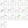 |
Fig. A.1. Hydrostatic mass radial profiles obtained from the forward method and the mass models applied to the backward method and described in Sect. 3.1. Vertical lines indicate: (dotted) R1000, R500, and R200; (dashed) third radial bin (a minimum number of three independent bins are needed to constrain a mass model with two free parameters) and upper limit in measurements of the spectroscopic temperature; (dot-dashed) radial range covered from SZ pressure profile after the exclusion of the three inner points and used in the reconstruction of the mass profile. Bottom panels: ratios of the different mass profiles to the NFW profile adopted as reference model. |
Appendix B: EG and MOND mass profiles
We present here the mass profiles for each X-COP object as obtained from (i) the backward NFW method, (ii) emergent gravity, and (iii) Modified Newtonian Dynamics.
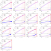 |
Fig. B.1. Hydrostatic, EG, and MOND mass radial profiles and relative ratios. Vertical lines indicate R1000 (dotted line), R500 (dash-dotted line), R200 (dashed line), and the outermost radial bin in the gas density profile (solid line). |
All Tables
Values of the total gravitating mass as estimated with the backward method and a NFW model at some radii of reference (0.5, 1, 1.5 Mpc) and at the overdensities of 500 and 200 with respect to the critical density of the universe at the cluster’s redshift.
For each mass model we have investigated (see Sect. 3.1), we quote the following best-fit parameters: scale radius rs (R200 in the case of NFW) and the concentration (or normalization) as defined in Eq. (3); the intrinsic scatter σT, int of Eq. (2); and the logarithmic value of the evidence E.
Values of χ2 (and relative degrees of freedom: d.o.f.) of the three components (emissivity ϵ, temperature T, and pressure P) of the likelihood presented in Eq. (2) and of the total χ2 for the best-fit mass model.
All Figures
|
Fig. 1. From top to bottom panels: reconstructed electron density, projected temperature, and SZ pressure profiles as functions of the radius in scale units of R500. Statistical error bars are overplotted. The two vertical lines indicate R500 and R200. |
| In the text | |
|
Fig. 2. Bayes factor of the mass models investigated with respect to the one with the highest evidence (see Table A.1). Shaded regions identify values of the Bayes factor where the tension between the models is either weak (< 2.5) or strong (> 5) according to the Jeffreys scale (Jeffreys 1961). |
| In the text | |
|
Fig. 3. Relative error (at 1σ) on the hydrostatic mass recovered with the backward method and a NFW model (see Table 1). |
| In the text | |
|
Fig. 4. Left panel: concentration–mass relation of the X-COP clusters. The dashed black lines show the median scaling relation (full black line) plus or minus the intrinsic scatter at redshift z = 0.06. The shaded grey region encloses the 68.3% confidence region around the median relation due to uncertainties on the scaling parameters. As reference, we plot the concentration–mass relations of Bhattacharya et al. (2013, blue line), Dutton & Macciò (2014, green line), Ludlow et al. (2016, orange line), and Meneghetti et al. (2014, solid and dashed red lines). The dashed red lines enclose the 1-σ scatter region in the theoretical concentration–mass relation from the MUSIC-2 N-body/hydrodynamical simulations. Empty circles identify the four objects (A644, A1644, A2255, A2319; see Fig. 2) for which NFW does not represent the best-fit mass model. Right panel: probability distributions of the parameters of the concentration–mass relation. The thick and thin black contours include the 1-σ and 2-σ confidence regions in two dimensions, here defined as the regions within which the probability is larger than exp(−2.3/2) and exp(−6.17/2) of the maximum, respectively. The red disk represents the parameters found by Meneghetti et al. (2014) for the relaxed sample. The bottom row plots the marginalized 1D distributions, renormalized to the maximum probability. The thick and thin black levels denote the confidence limits in one dimension, i.e. exp(−1/2) and exp(−4/2) of the maximum. |
| In the text | |
|
Fig. 5. Comparison between the backward NFW model and estimates of the mass from X-ray scaling relations (YX from Vikhlinin et al. 2009 – label on X-axis: |
| In the text | |
|
Fig. 6. Left panel: typical hydrostatic, EG and MOND radial mass profiles (here for A2142; plots for the remaining 12 objects in Appendix B. Vertical lines indicate R1000 (dotted line), R500 (dash-dotted line) and R200 (dashed line). Right panel: medians (and 1st and 3rd quartiles) of the ratio between the hydrostatic mass and the value predicted from EG and MOND for the whole X-COP sample. Shaded regions indicate the < 10% (darkest) and < 30% differences. |
| In the text | |
|
Fig. A.1. Hydrostatic mass radial profiles obtained from the forward method and the mass models applied to the backward method and described in Sect. 3.1. Vertical lines indicate: (dotted) R1000, R500, and R200; (dashed) third radial bin (a minimum number of three independent bins are needed to constrain a mass model with two free parameters) and upper limit in measurements of the spectroscopic temperature; (dot-dashed) radial range covered from SZ pressure profile after the exclusion of the three inner points and used in the reconstruction of the mass profile. Bottom panels: ratios of the different mass profiles to the NFW profile adopted as reference model. |
| In the text | |
|
Fig. B.1. Hydrostatic, EG, and MOND mass radial profiles and relative ratios. Vertical lines indicate R1000 (dotted line), R500 (dash-dotted line), R200 (dashed line), and the outermost radial bin in the gas density profile (solid line). |
| In the text | |
Current usage metrics show cumulative count of Article Views (full-text article views including HTML views, PDF and ePub downloads, according to the available data) and Abstracts Views on Vision4Press platform.
Data correspond to usage on the plateform after 2015. The current usage metrics is available 48-96 hours after online publication and is updated daily on week days.
Initial download of the metrics may take a while.