| Issue |
A&A
Volume 621, January 2019
|
|
|---|---|---|
| Article Number | A10 | |
| Number of page(s) | 14 | |
| Section | Extragalactic astronomy | |
| DOI | https://doi.org/10.1051/0004-6361/201732007 | |
| Published online | 20 December 2018 | |
Photoionization models for extreme Lyα λ1216 and Hell λ1640 line ratios in quasar halos, and PopIII vs. AGN diagnostics
1
Instituto de Astrofísica e Ciências do Espaço, Universidade do Porto, CAUP, Rua das Estrelas, Porto 4150-762, Portugal
e-mail: andrew.humphrey@astro.up.pt
2
Centro de Astrobiología (INTA-CSIC), Ctra de Torrejón a Ajalvir, km 4, Torrejón de Ardoz, Madrid 28850, Spain
3
Instituto de Astronomía, Universidad Nacional Autónomo de México, México Ap. 70-264, DF 04510, Mexico
4
Indian Institute of Technology Guwahati, Guwahati 781039, India
Received:
27
September
2017
Accepted:
5
October
2018
Aims. We explore potential mechanisms to produce extremely high Lyα/HeII flux ratios, or to enhance the observed number of Lyα photons per incident ionizing photon, in extended active galactic nucleus (AGN) photoionized nebulae at high-redshift.
Methods. We computed models to simulate, in the low density regime, photoionization of interstellar gas by the radiation field of a luminous AGN. We have explored the impact of ionization parameter, gas metallicity, ionizing spectrum, electron energy distribution, and cloud viewing angle on the relative fluxes of Lyα, HeII and other lines, and on the observed number of Lyα photons per incident ionizing photon. We have compared our model results with recent observations of quasar Lyα halos at z ∼ 3.5.
Results. Low ionization parameter, a relatively soft or filtered ionizing spectrum, low gas metallicity, κ-distributed electron energies, or reflection of Lyα photons by neutral hydrogen can all result in significantly enhanced Lyα relative to other lines (≥10%), with log Lyα/HeII reaching values of up to 4.6. In the cases of low gas metallicity, reflection by HI, or a hard or filtered ionizing spectrum, the observed number of Lyα photons per incident ionizing photon is itself significantly enhanced above the nominal Case B value of 0.66 due to collisional excitation, reaching values as high as 5.3 in an “extreme case” model which combines several of these effects. We find that at low gas metallicity (e.g. Z/Z⊙ = 0.1) the production of Lyα photons is predominantly via collisional excitation rather than by recombination. In addition, we find that the collisional excitation of Lyα becomes much more efficient if the ionizing continuum spectrum has been pre-filtered through an optically thin screen of gas closer to the AGN (e.g. by a wide-angle, feedback-driven outflow). We also show that the Lyα and HeII emission line ratios of a sample of previously studied quasars at z ∼ 3.5 are consistent with AGN-photoionization of gas with moderate to low metallicity and/or low ionization parameter, without requiring exotic ionization or excitation mechanisms such as strong line-transfer effects. In addition, we present a set of UV-optical diagnostic diagrams to distinguish between photoionization by Pop III stars and photoionization by an AGN.
Key words: galaxies: high-redshift / galaxies: abundances / galaxies: active / galaxies: ISM / quasars: emission lines / galaxies: halos
© ESO 2018
1. Introduction
The Lyman-alpha (Lyα λ1216) line of neutral hydrogen is an important observable in that it permits the discovery and study of galaxies at high redshift (e.g. Shibuya et al. 2018), particularly galaxies in a phase of star formation or active galactic nucleus (AGN) activity. This line is one of the intrinsically most luminous in galaxy spectra, but is relatively unstable as a quantitative diagnostic due to its resonant nature, and also due to its susceptibility to extinction by dust or other effects (e.g. Binette et al. 1993a). Despite its significant disadvantages, Lyα remains a key source of observational information about the evolution of galaxies and their gaseous environments across cosmic time (e.g. Haiman & Rees 2001).
Although typically less luminous and thus more difficult to observe, the non-resonant recombination line HeII λ1640 offers additional information to that provided by Lyα. Crucially, the ionization potential of He+ is far higher than that of H0 (54.4 vs. 13.6 eV) and the production of a significant flux of HeII relative to Lyα requires an ionizing source with a relatively hard ionizing spectrum, or else significant collisional ionization by shocks. Used together, Lyα and HeII offer potentially powerful diagnostics of the nature of ionizing sources in high-z galaxies, and a toolbox for understanding the physics of gaseous nebulae therein (e.g. Heckman et al. 1991; Villar-Martín et al. 2007; Arrigoni Battaia et al. 2015a; Feltre et al. 2016; Husemann et al. 2018; Dors et al. 2018).
One potentially powerful application of the Lyα to HeII flux ratio is in the identification of Population III (Pop III) stars in the high redshift Universe, by searching for HII regions or star forming galaxies with an emission line spectrum indicative of photoionization by an extremely hot thermal source (e.g. Schaerer 2002). However, care is needed to avoid misclassifying AGN as Pop III and vice versa (see e.g. Fosbury et al. 2003; Binette et al. 2003; Villar-Martín et al. 2004; Sobral et al. 2015, 2019; Bowler et al. 2016).
In addition, the Lyα to HeII flux ratio can inform us about the physics in nebulae associated with powerful AGN. For example, transfer effects and dust can strongly affect this line ratio (e.g. van Ojik et al. 1994; Villar-Martín et al. 1996), and photoionization modelling also suggests that the gas density and metallicity and the presence of young stars may also impact this line ratio in nebulae that are photoionized by an AGN (Villar-Martín et al. 2007).
Building on previous modelling (e.g. Villar-Martín et al. 1996, 2007; Arrigoni Battaia et al. 2015a,b), we present photoionization model calculations appropriate for large-scale Lyα nebulae photoionized by an AGN. In particular, we explore several potential mechanisms to produce “extreme” Lyα and HeII emission line ratios, or an enhancement in the number of Lyα photons per incident ionizing photon. In addition, we explore possible diagnostic diagrams to distinguish between photoionization by an AGN and photoionization by PopIII-like stars.
2. Defining “extreme” Lyα flux ratios
This study was motivated in part by the recent discovery by Borisova et al. (2016) of Lyα halos around a number of quasars at z ∼ 3.5, with Lyα λ1216/HeII λ1640 flux ratios that are typically significantly higher than those measured from the spatially integrated spectra of powerful radio galaxies at z > 2 (e.g. Vernet et al. 2001; Villar-Martín et al. 2007). Following Villar-Martín et al. 2007, we consider Lyα/HeII λ1640 > 15 (1.18 in log) to be an “extreme” ratio. This is above the normal range of values shown by high-z radio galaxies (see also De Breuck et al. 2000; Vernet et al. 2001), and above the range of values produced by ionization-bounded photoionization models that are able to reproduce the UV line ratios of z ∼ 2 radio galaxies (see, e.g. Villar-Martín et al. 1997, 2007).
3. Photoionization modelling
In order to examine how various physical conditions and the nature of the ionizing source can affect the emergent emission line spectrum of a photoionized nebula, we have computed a grid of photoionization models using the multi-purpose modelling code MAPPINGS 1e (Binette et al. 1985, 2012; Ferruit et al. 1997). Some regions of parameter space we investigate here have also been explored previously (e.g. Villar-Martín et al. 1996, 2007; Arrigoni Battaia et al. 2015a,b). Here we build on existing work by considering a wider range of parameter space, additional parameters, and previously unexplored combinations of parameters. Two-photon emission is present in all our models, due to the modelled plasma being in the low-density regime.
3.1. Fixed parameters
We keep several model parameters fixed throughout this study. For simplicity, we adopt an isochoric, plane-parallel, single-slab geometry. By default, the models are ionization-bounded unless otherwise stated, with computation terminated when the ionization fraction of hydrogen falls below 0.01.
3.2. Gas density nH
Throughout this paper, we define nH as the Hydrogen gas number density within our line emission models. Thus, all values of nH discussed herein are not necessarily directly equivalent to the volume-averaged gas densities which are often preferred when modelling large scale structure (e.g. Rosdahl & Blaizot 2012).
We have adopted 100 cm−3 as our default hydrogen number density, because we aim to simulate spatially extended, low density gas rather than compact regions of high density gas closely associated with the central AGN, whose gas clouds typically have nH > 1000 cm−3. To test the impact of lower gas density on the Lyα emission, we have computed additional models using nH = 0.1 cm−3, corresponding to the volume-averaged gas density in the outskirts of high-z quasar halos predicted by the numerical simulations of Rosdahl & Blaizot (2012).
3.3. Ionization parameter U
The ionization parameter1 U is effectively a measure of the ratio of ionizing photons to particles in the model gas cloud, and provides a useful parameterization of the ionization state of the gas. High-z Lyα emitters can be very large (r > 100 kpc), and there is a potentially very large range in U between individual objects and between different regions of objects, depending on r, Q, nH, etc. For example, a cloud of gas in the outer Lyα halo of a luminous quasar might have log U ∼ −3.5 (assuming Q ∼ 1056 s−1, r ∼ 100 kpc, nH ∼ 10 cm−3). A cloud closer to the quasar for instance might have log U ∼ −1.5 (with r ∼ 1 kpc, nH ∼ 1000 cm−3). On the other hand, a cloud might have log U ∼ −4.5 with nH ∼ 1 cm−3 at a distance of r ∼ 1 Mpc from a quasar. Thus, we should consider a suitably large range in U. Our model grid contains 100 values of U, starting at log U = −5 and ending at log U = 0.25. We increase U by +0.0531 dex (i.e., a factor of 1.13) between each model in the U-sequence to obtain a relatively fine sampling of this parameter.
3.4. Ionizing powerlaw index
By default, we adopt a power law with the canonical spectral index α = −1.5 (e.g. Robinson et al. 1987), where Sν ∝ ν+α (see also Telfer et al. 2002; Shull et al. 2012; Stevans et al. 2014). However, it has been suggested that AGN at high redshift (i.e., z ≳ 2) have a significantly harder ionizing spectrum (e.g. Francis 1993; Villar-Martín et al. 1997). On the other hand, it is conceivable that some active galaxies at high redshifts may instead have softer ionizing SEDs, due to the presence of a massive starburst which could contribute photons to the ionization of the extended Lyα halo (e.g. Villar-Martín et al. 2007), or perhaps due to partial filtering of the AGN’s ionizing continuum in a circumnuclear screen of gas (e.g. Binette et al. 2003). To test the impact of adopting a harder or softer powerlaw, we have also computed model sequences using α = −1.0 or α = −2.0.
3.5. Gas chemical abundances
We also vary the gas chemical abundances, to examine the impact of metallicity on the emergent emission line spectrum. As the starting point for the chemical abundance sets considered here, we adopt the Solar chemical abundances as determined by Asplund et al. (2006). For non-Solar gas abundances, we scale all metals linearly.
Lyα emitting regions associated with galaxies at high-z have a potentially very large dispersion in gas metallicity, ranging from extremely metal poor gas on the outskirts of a very young galaxy at high redshift, to metal-enriched gas close to the active nucleus of a massive galaxy. Thus, we consider three representative gas metallicities of Z = 0.01, 0.10, and 1.0 times the Solar metallicity (Z⊙).
3.6. Electron energy distribution and κ
Among the novel features of MAPPINGS 1e is the ability to use the non-equilibrium, Kappa-distribution (KD) of electron energies instead of the commonly adopted Maxwell–Boltzmann distribution (MBD). The KD of electron energies used in MAPPINGS 1e is a function of electron temperature and the κ parameter, where 1.5 < κ < ∞, and is described in Nicholls et al. (2012; see also Vasyliunas 1968). When κ → ∞, the distribution becomes a MBD. Full details of the implementation of KD electron energies in MAPPINGS 1e are given in Binette et al. (2012).
Although the physics underpinning the KD is not yet fully understood (see, e.g. Ferland et al. 2016; Draine & Kreisch 2018), the presence of KD energies in Solar System plasmas is well established (e.g. Vasyliunas 1968; Livadiotis & McComas 2011; Livadiotis 2018). Thus, it is important to consider the possibility that KD electron energies may be present in some extrasolar and extragalactic plasmas. Indeed, a number of recent studies have shown that many commonly observed nebular emission lines can be significantly affected by adopting the KD, both in HII regions and high-z radio galaxies, and the KD has been proposed as a solution to the long-standing observational temperature discrepancies in planetary nebulae and HII regions (Nicholls et al. 2012, 2013; Binette et al. 2012; Humphrey & Binette 2014).
Values in the range 10 ≲ κ ≲ 40 have been proposed for HII regions and planetary nebulae (e.g. Nicholls et al. 2012; Binette et al. 2012) and AGN (Humphrey & Binette 2014), where a smaller κ represents a stronger deviation from the MBD. In this Paper we consider κ = 20 in place of the MBD distribution in some model sequences.
3.7. Cloud viewing angle
As previously shown by Villar-Martín et al. (1996), neutral hydrogen at the back of the cloud can act as a “mirror” to back-scatter Lyα towards the front of the cloud, enhancing the flux of Lyα as seen by the observer, relative to other lines. To avoid confusion with other geometrical set-ups, we refer to this neutral “mirror” at the rear of the cloud as a “back-mirror”.
We consider two viewing angles for the model cloud (slab). By default, we have adopted the “side view”, which places the observer at an angle of 90° to the direction of travel of the incident ionizing radiation. In addition, we also calculate the “front view”, where the observer views the illuminated face of the cloud (see Binette et al. 1993a,b). In all of our ionization-bounded models, the column density of neutral hydrogen towards the back of the cloud (NHI ≥ 1018 cm−2) is substantially higher than what is required to produce a significant neutral “back-mirror” effect (the minimum required is NHI ≳ 1014 cm−2). This “back-mirror” effect would be much weaker in models in which the illuminated gas is optically thin to ionizing radiation (matter-bounded), such as the filtering screen described in Sect. 3.8 below, or the optically thin photoionization models that Arrigoni Battaia et al. (2015b) favoured in explaining the Lyα emission from the giant gas halo of the z = 2.28 quasar UM287.
To reflect Lyα photons from the active nucleus (whether hidden or viewed directly), such neutral “back-mirrors” as considered here are not strictly needed. This is because even a matter-bounded HII slab of reasonable opacity (e.g. Binette et al. 1996) will have a non-negligible HI fraction and thus can scatter to our line-of-sight Lyα photons from the active nucleus (e.g. Humphrey et al. 2013a; Cantalupo et al. 2014), potentially providing a further enhancement to the flux of Lyα. However, we do not consider this additional effect here.
3.8. Ionization by a filtered SED
We also study the impact of photoionizing gas clouds using an ionizing powerlaw SED that has first been filtered through a screen of gas that does not fully absorb all ionizing photons. A situation where this might occur would be in a galaxy which contains a wind-blown superbubble that is expanding into the extended gaseous halo (e.g. Tenorio-Tagle et al. 1999; Taniguchi et al. 2001). In this case, one would expect the bubble to partially filter the AGN’s ionizing continuum so that gas clouds at radii beyond the bubble would see an altered version of the ionizing SED. Alternatively, the ionizing spectrum of the AGN might be filtered by gas in the host galaxy, before escaping to ionize gas on hundreds of kpc scales, giving essentially the same result. Several previous studies have addressed this issue (see e.g. Binette et al. 1996, 2003), and among the main effects are lower fluxes for HeII and other high-ionization lines, and lower electron temperatures, than would have resulted using the original (unfiltered) SED.
Here, we look specifically at the impact of a filtered ionizing SED on Lyα flux ratios. For this, we have produced a set of four filtered SEDs by computing matter-bounded photoionization models with α = −1.5, log U = −2 and NH = 1.0, 2.5, 5.0 or 7.0 × 1020 cm−2, giving ionizing continuum escape fractions of Fesc = 0.90, 0.74, 0.50 and 0.28, respectively2. The choice of values for U and NH are not critical, and can be scaled in lockstep to produce a similar emergent distribution. The metallicity of the screening gas is assumed to be solar. The resulting ionizing SEDs were then used as inputs for new, U-sequence model calculations.
The various filtered SEDs are shown in Fig. 1. The main dips seen in our filtered SEDs are caused by photoelectric absorption of photons by H (13.6 eV) and He+ (54.4 eV), resulting in a spectrum with a comparatively lower number of He+ ionizing photons. For comparison, we also show the residual of an α = −1.5 ionizing SED from an unfiltered model calculation.
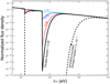 |
Fig. 1. Filtered AGN spectral energy distributions described in Sect. 3.8. These correspond to escape fractions of 0.28 (solid black line), 0.50 (solid red line), 0.74 (solid blue line) and 0.90 (solid cyan line). For comparison, we also show the emergent distribution from a typical ionization-bounded model (dashed black line): the UV part of the spectrum has been completely absorbed, while some X-rays still escape through the cloud. The vertical axis (normalized flux density or Sν) gives the power per unit area per unit frequency in arbitrary units. The escape fractions are in photon number flux, while the SEDs are plotted in energy flux per unit frequency (Sν). |
When computing models using a filtered SED, we have scaled by Fesc the range in U values covered. For instance, when using our Fesc = 0.28 SED, our U-sequences run from log U = −4.55 to log U = −0.30. This introduces a differential shift in the curves that are plotted as a function of U. To facilitate visual comparison between models, we show in Appendix A the same models as a function of U⋆ = U/Fesc.
We do not include line emission produced within the filtering screen in the resulting line fluxes from our filtered continuum models. The relative significance of the line flux from the absorbing screen depends strongly on its physical conditions, and can varies from significant when the screen and post-screen gases have similar physical conditions (see the models of Binette et al. 1996), to negligible as in the case where the filtering screen is obscured (from the observer) by nuclear dust. A full treatment of the emission from such a screen is beyond the scope of this paper.
3.9. Ionization by Pop III stars
We also include a model sequence to simulate a low-metallicity nebula being photoionized by Pop III (or Pop III-like) stars, with the aim of understanding to what extent their Lyα flux ratios differ from those of our AGN models. Taking into account the effect of He+ opacity, a zero-metallicity star with an effective temperature of 80 000 K would be equivalent to a black-body of 67 200 K in terms of the proportion of He+-ionizing photons (see Holden et al. 2001; Schaerer 2002; Binette et al. 2003). Thus, we adopt a black-body temperature of 67 200 K in this model sequence.
We also use a gas phase metallicity of Z/Z⊙ = 0.01, to account for some slight pollution with metals, and for consistency with the low-metallicity AGN powerlaw models against which our Pop III models will be compared. For easy comparison with our AGN models, our Pop III models use an ionization-bounded, plane-parallel geometry and nH = 100 cm−3.
It is not our intention to model in detail the expected line spectrum of a Pop III-ionized nebula, but to reach a general overview of the potential for such a nebula to be confused with an AGN-photoionized nebula when only the strongest UV emission lines are available. We stress that this model sequence may be unrealistic in that true Pop III stars are expected to form from chemically primordial gas, with the associated HII region being similarly devoid of metals. Our model sequence, however, does consider a zero-metallicity Pop III star (or stars), but the gas it photoionizes has already undergone some slight polution with metals. In a future paper we will present a more detailed modelling of emission line diagnostics for Pop III HII-regions and Pop III galaxies.
4. Results
Here we describe the results from our model grid using diagnostic diagrams, which we show in Figs. 2–7.
 |
Fig. 2. Selected sequences in U plotted for Lyα/HeII vs. Lyα/Hβ, Lyα/Hα, Hα/Hβ, or [OIII] λ5007/Hβ. Each sequence represents a progression in U, for each of the three values of Z. Also shown are sequences in U using κ = 20 for Z/Z⊙ = 0.01 and 1.0 (dotted curves). All models in this figure use power index α = −1.5. The lower two panels show Lyα/HeII vs. U (left) and the ratio of Lyα photons to ionizing photons (ηLyα; right) for the same model sequences. The model loci cover the range of ionization parameter −5 < log U < 0.25. |
4.1. AGN models – line ratios
Our modelling shows that “extreme” ratios of Lyα/HeII can be readily produced using AGN photoionization. Within our model grid this flux ratio spans a huge range in values, from log Lyα/HeII ∼1.1 to ∼4.6, without the need to invoke physically implausible values for model parameters. Below we describe the impact of individual parameters on the line ratios, giving examples to quantify the impact at specific positions within our parameter space.
We find that Lyα/HeII is extremely high when U is relatively low, regardless of which electron energy distribution and gas metallicity are selected, as can be seen in Fig. 2. For example, at Z/Z⊙ = 0.1 and log U = −4 we obtain log Lyα/HeII = 1.88. There is essentially no upper limit to the Lyα/HeII flux ratio, with Lyα/HeII → ∞ as U → 0 (log U → −∞). We also note that most of the model sequences show at their high-U end (log U ≳ −2.5) a region of relatively constant Lyα/HeII values, confirming that this ratio is relatively insensitive to U in the high-ionization regime (Fig. 2; see also e.g. Villar-Martín et al. 2007; Arrigoni Battaia et al. 2015b).
As shown by previous authors, a reduction in gas metallicity results in enhanced emission of Lyα relative to HeII due to increased collisional excitation of Lyα resulting from the increase in electron temperature (e.g. Villar-Martín et al. 2007). As shown in Fig. 2, our models indicate that this effect can also strongly enhance Lyα/Hβ. On the other hand, Hα/Hβ and Lyα/Hα show relatively small increases with reducing metallicity. For instance, when log U = −2 and α = −1.5, moving from Z/Z⊙ = 1.0 to Z/Z⊙ = 0.1 changes log Lyα/HeII from 1.25 to 1.46 (+0.21 dex); log Lyα/Hβ from 1.43 to 1.59 (+0.16 dex); Lyα/Hα from 0.96 to 1.10 (+0.14 dex); Hα/Hβ from 0.46 to 0.49 (+0.03 dex).
The impact of using the κ-distribution is complex and varies across the range in parameter space we examine in this work. Generally speaking, using κ = 20 results in a minor enhancement of Lyα relative to HeII, Hβ and Hα at high metallicity (Z/Z⊙ ≳ 1.0), but when metallicity is low (Z/Z⊙ ≲ 0.1) the Lyα is marginally reduced relative to those lines. For instance, at log U = −2, α = −1.5 and Z/Z⊙ ≳ 1.0, log Lyα/Hβ changes from 1.43 to 1.46 (+0.03 dex) when adopting κ = 20, but at Z/Z⊙≳0.1 we find that using κ = 20 reduces log Lyα/Hβ from 1.59 to 1.58 (−0.01 dex). In other words, the impact on Lyα of adopting a κ-distribution with κ = 20 is marginal to insignificant, at least in the range of parameter space we consider herein. A full analysis of the impact of using the KD in place of the MBD on the emergent spectrum of active galaxies and high-z Lyα emitters will be presented in a future Paper (Morais et al., in prep.).
Figure 3 shows the impact of using different ionizing spectral indices (α). As expected from previous studies (e.g. Humphrey et al. 2008; Arrigoni Battaia et al. 2015b), the Lyα/HeII flux ratio is higher when using a softer ionizing spectrum, because there are relatively fewer photons able to ionize He+ (hν > 54.4 eV). However, a softer ionizing SED results in a reduction in the flux of Lyα relative to Hβ and Hα, and a reduction in Hα/Hβ, because a softer SED results in lower electron temperatures, reducing the importance of collisional excitation effects on these lines. For instance, at log U = −2 and Z/Z⊙, we find that moving from α = −1.0 to α = −2.0 changes log Lyα/HeII from 1.17 to 1.44 (+0.27 dex), log Lyα/Hβ from 1.59 to 1.37 (−0.22 dex), log Lyα/Hα from 1.11 to 0.91 (−0.20 dex), log Hα/Hβ from 0.48 (3.04) to 0.45 (2.84), and < TOIII > from 14700 K to 9200 K.
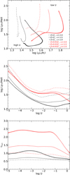 |
Fig. 3. Impact of the powerlaw index of the ionizing spectrum on Lyα/HeII, Lyα/Hβ and ηLyα. The model loci cover the range of ionization parameter −5 < log U < 0.25. |
In Fig. 4 we show the effect of adopting the “front view” in our adopted geometry. In our models, the observed flux of Lyα (relative to other lines) is nearly twice that of the “side view”, with HI in the partially ionized or neutral zone reflecting almost all of the incident Lyα emission, close to the factor 2.0 (0.3 dex) theoretical maximum effect for a uniformly flat “back-mirror” with a covering factor of unity. Interestingly, Fig. 4 also reveals a degeneracy between metallicity and cloud viewing angle, with the “front view” mimicking models that use the “side view” with a lower gas metallicity. Conversely,“rear view” models (not shown) result in much lower Lyα flux relative to most other lines, as there is no direct Lyα.
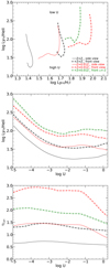 |
Fig. 4. Impact of viewing angle on the observed Lyα/HeII, Lyα/Hβ and ηLyα values. The green curve shows the locus of our sequence in U using Z/Z⊙ = 0.01, α = −2.0 and the “front view”, to illustrate the combined effect of low U, low gas metallicity, a relatively soft ionizing continuum, and a “back-mirror”. The model loci cover the range of ionization parameter −5 < log U < 0.25. |
As expected, using a filtered ionizing SED results in an enhancement of Lyα/HeII compared to the original, unfiltered SED (Fig. 5). This is primarily because the absorbing screen preferentially absorbs photons in the range 54.4–200 eV, reducing the relative number of photons that can ionize He+ (hν ≥ 54.4 eV) compared to H (see Fig. 1). The enhancement in Lyα/HeII is also partly due to increased collisional excitation of Lyα (see discussion of ηLyα in Sect. 4.2), via two different effects: (i) Collisional excitation of Lyα requires the presence of neutral H; because it is relatively harder than the unabsorbed powerlaw, the filtered SED is less efficient at ionizing H, resulting in a higher H neutral fraction and thus a higher rate of collisional excitation of Lyα; (ii) Photoionization by the filtered (harder) SED produces photoelectrons that are on average more energetic, increasing the heating rate and temperature of the gas, again leading to a higher rate of collisional excitation of Lyα. To corroborate the presence of these effects, we show in Table 1 the Lyα/HeII ratio and its relation to gas metallicity, electron temperature, and choice of SED. Even though using a filtered continuum does not always result in a higher average electron temperature, it does increase the Balmer decrement, indicating the increased importance of collisional excitation.
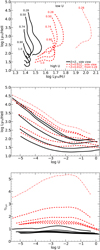 |
Fig. 5. Impact of using a filtered ionizing continuum instead of a simple powerlaw on the observed values of Lyα/HeII, Lyα/Hβ and ηLyα. U-sequences using a filtered ionizing continuum are labelled with their value of Fesc. U-sequence loci which use our default powerlaw of α = −1.5 are labelled “1.0” because the input SED is unfiltered. The dot-dashed curve (on the right of the upper panel) shows the locus of our sequence in U that uses Fesc = 0.28, Z/Z⊙ = 0.01, α = −1.5 and the “front view”, to illustrate the combined effect of low U, low gas metallicity, a heavily filtered ionizing continuum, and a “back-mirror”. For each combination of U and Z/Z⊙, a lower Fesc results in lower Lyα/HeII and higher ηLyα. In Fig. A.1 we show an alternate version of this Figure, plotted with U scaled by 1/Fesc to aid comparison with our other models. |
Illustrating the impact of low gas metallicity and/or a filtered ionizing SED on the production of Lyα.
The impact on Lyα/HeII can be large, even when the filtering screen has a high escape fraction. For example, using our Fesc = 0.90 SED we obtain a Lyα/HeII ratio that is ∼0.2 dex higher than the unfiltered SED. Even for Fesc as high as ∼0.97 (not shown here), this line ratio is still significanly enhanced (+0.04 dex or 10 percent). At the other end of the parameter range, we obtain log Lyα/HeII = 4.4 using the Fesc = 0.28 SED, Z/Z⊙ = 1.0 and log U = −5, which rises to 4.6 if we also include the effect of a “back-mirror”. Using a filtered SED also results in slight increase in Lyα/Hβ, of up to ∼0.1 dex in the extreme case of our Fesc = 0.28 SED. We also note that lower ionization lines tend to become stronger relative to high-ionization lines and HeII (see e.g. Binette et al. 2003).
We find that gas density has a small, but potentially significant effect on the ratios Lyα/HeII when log U ≲ −2 and Z/Z⊙ = 1.0 (Fig. 6). In this parameter range, Lyα/HeII is up to 0.1 dex higher when using nH = 100 cm−3 as compared to an equivalent nH = 0.1 cm−3 model. However, at higher values of U, or at low gas metallicity (Z/Z⊙ ≤ 0.1), we find no significant difference in the Lyα/HeII ratio between our nH = 0.1 and nH = 100 cm−3 models.
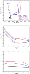 |
Fig. 6. Impact of gas density on the observed Lyα/HeII, Lyα/Hβ and ηLyα values. The model loci cover the range of ionization parameter −5 < log U < 0.25. |
We note that combining several of the above effects can have a cumulative enhancement on the Lyα/HeII ratio. This is clearly evident in Figs. 2–5. For instance, we find that photoionization at low U (e.g. log U ≲ −5) by a moderately filtered continuum (e.g. Fesc ≲ 0.5) can result in very extreme Lyα/HeII flux ratios, with log Lyα/HeII ≳ 4 (Fig. 5). In another extreme case from our model grid, we see that low gas metallicity (Z/Z⊙ = 0.01), a relatively soft SED (α = −2.0) and low ionization parameter (log U = −5) together result in log Lyα/HeII = 2.88 and log Lyα/Hβ = 1.88 (Fig. 3).
4.2. AGN models – Lyα to ionizing photon ratio
It is also interesting to consider how the luminosity of the Lyα line varies across our grid of models. To simplify the comparison between models we use ηLyα, the ratio of emergent Lyα photons to incident ionizing photons. Figures 2–5 each include a panel showing ηLyα vs. log U. Our fiducial model sequence using α = −1.5 and Z/Z⊙ = 1 (Fig. 2) produces values of ηLyα that are close to the value ηLyα = 0.66 expected for complete absorption of the incident ionizing spectrum and purely recombination emission from gas which is optically thick in the Lyman line series (Case B; e.g. Gould & Weinberg 1996). However, we find significant variation in ηLyα across our model grid, which we describe below.
As shown in Fig. 2 (lower right), the gas metallicity can have a strong effect on ηLyα, with lower metallicities resulting in higher values of ηLyα (see also Table 1). For instance, reducing Z/Z⊙ from 1 to 0.01 increases ηLyα by a factor of ∼2. Interestingly, some of our model loci show a substantial drop in ηLyα at higher values of U (log U ≳ −2), particularly in model sequences which use low gas metallicity (Z/Z⊙ ≤ 0.1) and a hard ionizing SED (α ≥ −1.5; see, e.g. Fig. 3). Interestingly, when the gas metallicity is sufficiently low (Z/Z⊙ = 0.01), the rate of collisional excitation3 can become the dominant channel for the production of Lyα photons, i.e., at ηLyα ≳ 1.4.
Figure 2 (lower right) also reveals that the choice of electron energy distribution can also have a significant impact on ηLyα. At high gas metallicity (Z/Z⊙ = 1), we find that using κ = 20 instead of the MBD results in a ∼10–20 percent enhancement of ηLyα in the range −5 < log U < −2. However, at low gas metallicity (i.e., Z/Z⊙ = 0.01), our κ-distribution models do not show any significant enhancement in ηLyα, instead showing a ∼10 percent reduction in ηLyα at log U > −1.4, with no significant difference from the equivalent MBD models when log U < −1.4.
The hardness of the ionizing radiation also has an impact on ηLyα (Fig. 3), with harder ionizing spectra (higher α) resulting in higher values of ηLyα. As an example of this, our models with α = −1.0 and Z/Z⊙ = 1 yield values of ηLyα that are up to ∼4 times higher than produced in our α = −2.0 Z/Z⊙ = 1 models. This difference widens at lower metallicity: at the low-metallicity end of our grid (Z/Z⊙ = 0.01), we find that ηLyα is a factor of up to ∼30 higher when using α = −1.0, compared to α = −2.0.
These enhancements of ηLyα above the expected Case B value are primarily driven by collisional excitation of Lyα at the enhanced electron temperatures that result from using lower gas metallicity, a harder ionizing spectrum and/or κ-distributed electron energies. The higher neutral H fraction produced by the filtered SED can also result in a higher rate of collisional excitation of Lyα. As a quantitative illustration of this effect, when using α = −1.5 and log U = −2 we find the average electron temperature in the H+ zone is T = 11 605 K when Z/Z⊙ = 1, compared to T = 21 383 K at Z/Z⊙ = 0.01, resulting in ηLyα = 0.68 and ηLyα =1.40, respectively (see also Table 1).
In addition, we find that using a filtered ionizing spectrum (Fig. 5) results in an increased ηLyα, with more strongly filtered spectra producing higher values of ηLyα. This is primarily due to the increased importance of collisional excitation under such conditions. This effect also results in an increased Balmer decrement (see Table 1).
Although technically not an enhancement in ηLyα, the inclusion of the effect of a “back-mirror”, with the cloud viewed from the front, does also increase the apparent (or observed) ηLyα by a factor of ∼2 (Fig. 4). We find no significant difference in ηLyα between our nH = 0.1 and nH = 100 cm−3 models (Fig. 6).
In summary, we find a substantial variation in ηLyα, the ratio of Lyα photons to incident ionizing photons, across our AGN photoionization model grid. In particular, there is a substantial deviation from the case B recombination value ηLyα = 0.66. In our grid, ηLyα ranges from a minimum value of ηLyα = 0.58 in the case of solar metallicity gas illuminated by a powerlaw with α = −1.5 at log U = 0.25, to a maximum of ηLyα = 2.7 for a gas cloud with Z/Z⊙ = 0.01 illuminated at U = −1.6 by our Fesc = 0.28 filtered SED. If we also include a neutral “back mirror”, then the maximum (effective) value in our grid is ηLyα = 5.3 (see Fig. 5).
4.3. Degeneracy between AGN and black-body models
Figure 7 shows a comparison between our Pop III U-sequence and AGN U-sequences with the following parameters: (1) α = −1.5; (2) α = −1.5 with the “front view” of a photoionized slab with a “back-mirror”; (3) α = −2.0; (4) photoionization by an α = −1.5 powerlaw that has been filtered such that Fesc = 0.50. All the models use Z/Z⊙ = 0.01.
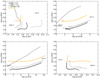 |
Fig. 7. Diagnostic diagrams comparing Pop III (heavy orange line) and several AGN photoionization models. The AGN model U-sequences shown here are: α = −1.5 (thick black line); α = −2.0 (thin black line); α = −1.5 with “front view” (“back-mirror”) (dot-dashed line); photoionization by our Fesc filtered AGN continuum (dashed line). All models shown in this figure use Z/Z⊙ = 0.01. See main text for further details. The model loci cover the full range of ionization parameter in our model grid, i.e., −5.55 < log U < 0.25. |
Comparing models with identical values of U, we find that the Pop III models give Lyα/HeII ratios that are around one order of magnitude higher than in the powerlaw AGN models. Nonetheless, three of the AGN sequences do show an overlap in Lyα/HeII with the Pop III sequence. The low-U ends of the α = −2.0 and the α = −1.5 “front view” sequences reach up above log Lyα/HeII ∼ 2.5, while the Fesc = 0.50 filtered continuum model overlaps with the full range of Lyα/HeII values in the Pop III model sequence. In other words, it is not possible to distinguish between photoionization by an AGN or by Pop III stars on the basis of the Lyα/HeII ratio alone4.
However, the addition of a second line ratio eases the degeneracy between our model sequences. Of the four diagnostic diagrams shown in Fig. 7, the diagram showing Lyα/HeII vs. Lyα/Hβ yields the cleanest separation of models, with the AGN sequences falling below and/or to the right of the Pop III model sequence, because their ionizing SEDs contain a higher proportion of He+ ionizing photons, and/or because the ionized gas has a higher Te. This diagram also provides a clear diagnostic to distinguish cases of ionization by a relatively soft source (e.g. Pop-III stars of an α = −2.0 powerlaw) from AGN-photoionization by an α = −1.5 powerlaw with enhanced Lyα emission due to scattering effects (e.g. our “front view” models). Using a softer ionizing SED shifts a model upwards, while scattering-enhanced Lyα shifts a model up and right.
The other three diagnostic diagrams in Fig. 7 show Lyα/HeII vs. Lyα/CIV λ1549, Lyα/CIII] λλ1907,1909 and Lyα/CII] λ2326. There is a relatively clean separation between the Pop III sequence and the power-law AGN models, which run roughly parallel to each other. Only at their very low-U end do the α = −2.0 and “front view” model sequences cross the locus of Pop∼III models. Interestingly, the filtered AGN continuum sequence crosses the Pop III sequence in all three of our Lyα to carbon diagrams, indicating a degeneracy between these two types of model when Lyα/HeII is used together with ratios involving CIV, CIII] and/or CII] (see also Fosbury et al. 2003; Binette et al. 2003).
5. Discussion
Recently, Borisova et al. (2016) discovered ubiquitous, large-scale Lyα emitting halos around 19 quasars at z ∼ 3.5. Interestingly, the authors found extreme Lyα/HeII flux ratios in 11 of the 19 halos, typically with higher Lyα/HeII ratios than in high-redshift radio galaxies.
A number of earlier observational studies have also detected extremely high Lyα/HeII flux ratios in extended Lyα-emitting regions around distant AGN, with proposed explanations including enhanced Lyα flux due to the resonance scattering reflection of Lyα by a large-scale unform halo of neutral or possibly matter-bounded gas (see Sect. 3.7), or recombination emission resulting from photoionization of metal-poor gas by the AGN, (e.g. Villar-Martín et al. 2007; Humphrey et al. 2013a; Arrigoni Battaia et al. 2015b).
Our modelling has confirmed that scattering effects can indeed lead to up to a factor of ∼2 enhancement of Lyα/HeII, under circumstances that may plausibly be present in the Lyα nebulae of some high-z AGN (see also, e.g. Villar-Martín et al. 1996). However, our models also show that photoionization by an AGN can produce extreme values of Lyα/HeII even without Lyα scattering effects. These include low gas metallicity, a soft or filtered ionizing SED, or a low ionization parameter.
In Fig. 8 we show a selection of relevant photoionization models from our grid, together with the Lyα/HeII flux ratios of Borisova et al. (2016)5. A horizontal line at log Lyα/HeII = 1.18 delineates the “extreme” and “normal” Lyα/HeII regimes defined in Sect. 2.
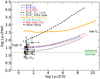 |
Fig. 8. Lyα/HeII vs. Lyα/CIV showing the locus of several of our photoionization model sequences, along with the measurements or 3σ lower limits on these ratios taken from the Lyα halos of z ∼ 3.5 quasars of Borisova et al. (2016). The model loci cover the full range of ionization parameter in our model grid, i.e., −5 < log U < 0.25. The horizontal green dotted line marks the boundary between what we define as “extreme” and “normal” Lyα/HeII flux ratios. |
Interestingly, all of the ionization models shown in Fig. 8 lie within the “extreme” regime, although at high U the Z/Z⊙ = 1.0, α = −1.5 curve comes close to the boundary6. Thus, we argue that unless log U ≳ −2.5 and Z/Z⊙ ∼ 1, one should expect the intrinsic (emitted) Lyα/HeII ratios of quasar-photoionized halos to be well within the “extreme” regime. We also suggest that for a quasar-ionized halo to appear well inside the “normal” regime (log Lyα/HeII ≲ 1), its Lyα emission would need to be either strongly absorbed, or else would need to contain a substantial population of matter-bounded clouds that are sufficiently thin for He to be mostly doubly-ionized.
The majority of the quasars in the sample of Borisova et al. (2016) have only lower limits on Lyα/HeII and Lyα/CIV. Unfortunately, these limits are consistent with essentially all of the models we have considered, and thus we cannot place meaningful constraints on properties such as U, Z, α, etc. for the gas halos of these particular quasars.
Only two quasars in the sample of Borisova et al. (2016) have detections of narrow HeII, and both show large vertical offsets of ∼0.3 dex from our AGN powerlaw models. One of these quasars, PKS 1937–101 at z = 3.77, shows log Lyα/HeII = 0.92, placing it within the “normal” Lyα/HeII regime in Fig. 8 (red data point). Its position ≳0.2 dex below all of our models (including our Z/Z⊙ = 1.0, α = −1.0 models) suggests that this quasar halo suffers from strong absorption of Lyα (NHI ≳ 1014 cm−2), is ionized by an unusually hard SED (i.e., α < −1.0), or is composed of matter-bounded clouds rather than the ionization-bounded clouds modelled here.
The other quasar from this sample with a detection of both HeII and CIV is CTS R07.04, at z = 3.35 (cyan point in Fig. 8). Its Lyα halo has log Lyα/HeII ∼ 2 and log CIV/HeII ∼ 5, placing it ≳0.4 dex above our powerlaw AGN model loci, but very close to our Z/Z⊙ = 1.0, Fesc = 0.50 filtered continuum model locus. We suggest that this quasar halo is ionized by an unusually soft SED (for an AGN), due to strong filtering of the quasar’s SED by a screen of gas closer to the nucleus, perhaps due to a wide-angle, AGN-driven outflow closer to the nucleus of the galaxy itself. Alternatively, in the case of this quasar one could suppose the presence of a significant contribution from an ionization mechanism that does not produce strong HeII, such as cooling radiation or photoionization by hot, young stars.
With the probable exception of CTS R07.04, we find no need for subsolar gas metallicites, a soft ionizing continuum (including PopIII stars), or enhanced Lyα by scattering to reproduce the Lyα/HeII flux ratios. However, strictly speaking these are not ruled out.
As a consistency check, we can calculate the Lyα luminosity expected from the implied value of U and the observed size of a Lyα halo, and then compare against observed values of Lyα luminosity from Borisova et al. (2016). For photoionization of gas the expected Lyα luminosity is given by:

where fc is the covering factor of the gas as seen by the ionizing source, nH (cm−3) is the gas density, U is the ionization parameter, r (cm) is the distance of the cloud from the ionizing source, ηLyα is the ratio of emitted Lyα photons to incident ionizing photons (see Sect. 4.2), and Ω is the solid angle (in sr) of the central source covered by the ionized gas7. The factor 0.5 arises from the multiplication of the constants 4π, hνLyα, c, and 1/4π sr. Due to the expected uncertainty in the values of nH, fc and ηLyα, we expect uncertainties in resulting estimates of LLyα to be at least a factor of ∼10. Throughout this work, we assume that the ionizing radiation of the AGN is beamed into a bicone covering a solid angle of Ω = 3.7 sr, corresponding to a pair of ionization cones, each with an opening angle of 90°.
Taking one of the most “extreme” cases from Borisova et al. (2016), Q0042–2627 (z=3.3), its Lyα/HeII ratio >67 (1.8 in log) would require log U ≲ −4.2 in our Solar metallicity, α = −1.5 powerlaw model sequence, corresponding to ηLyα ∼ 0.66 (determined from Fig. 2). Although there is likely to be some radial evolution in one or more of U, nH, and fc, the exact behaviour of these parameters in a real halo is far from clear. Thus, we adopt constant but characteristic values for each of them. Adopting nH = 100 cm−3 and fc ∼ 0.1 estimated from radio-loud, type 2 quasars at z ≳ 2 (e.g. McCarthy 1993; Villar-Martín et al. 2003), assuming Ω = 3.7 sr, and using the maximum observed radius of Lyα emission r = 4.9 × 1023 cm (160 kpc) from Borisova et al. (2016), we estimate LLyα ≲ 1.8 × 1044 erg s−1 – consistent with the observed luminosity LLyα=1.7 × 1044 erg s−1 in Table 2 of Borisova et al. (2016). The resulting ionizing luminosity of the AGN would be Q ≲ 6 × 1056 s−1. The values of LLyα and Q we have derived are both upper limits because our estimate of U, from which both are derived, is also an upper limit.
Using instead our model sequence with Z/Z⊙ = 0.1 and α = −1.5, we find log U ≲ −3.8 and ηLyα ≲ 1.25 from Fig. 2. Leaving r, nH, fc and Ω unchanged, we obtain LLyα ≲ 9 × 1044 erg s−1 – still consistent with the observed luminosity. Using the same methodology, we also find a similar level of consistency between the expected and observed LLyα values for the 10 other quasars from Borisova et al. which show “extreme” Lyα/HeII ratios.
These calculations serve to illustrate the plausibility of very low U, possibly coupled with low gas metallicity, to explain the “extreme” Lyα/HeII ratios measured by Borisova et al. (2016). However, we stress that our consistency check is not intended as proof of a particular value for any of the parameters in Eq. (1).
It seems particularly plausible that the large-scale gas halos of high redshift quasars such as these would have low gas metallicity, since the central galaxy is expected to be fed by cold streams of pristine or very low metallicity gas from the cosmic web (e.g. Goerdt et al. 2015; Vernet et al. 2017). However, observations of the halos of high-z quasars appear to show such halos are already polluted with metals (e.g. Humphrey et al. 2013a; Prochaska et al. 2013).
The detectability of Lyα from extended gas around high-z AGN, and the use of this emission for improving our understanding of galaxy evolution, continue to be key topics in extragalactic astrophysics (e.g. Haiman & Rees 2001; Villar-Martín et al. 2003; Borisova et al. 2016). Our new modelling results have interesting implications for the detectability of Lyα halos associated with high-z AGN. Firstly, cold gas around a quasar should be considerably more luminous in Lyα, and thus easier to detect, if the gas has a lower metallicity and/or if it sees a harder ionizing spectrum. We also suggest that the high detection rate of extended Lyα halos in quasars at high-z (e.g. Borisova et al. 2016) may be due to this effect. In addition, lower gas metallicity and a harder ionizing spectrum could result in apparently larger Lyα halos, as the correspondingly higher ηLyα would make faint, outer regions more detectable.
6. Summary
We have used the modelling code MAPPINGS 1e to explore potential mechanisms to produce enhanced Lyα relative to HeII and other emission lines in extended nebulae photoionized by powerful AGN. Our grid of photoionization models cover a substantial range in ionization parameter U, the gas metallicity and the shape of the ionizing continuum, and considers two different electron energy distributions and cloud viewing angles.
We are able to produce “extreme” Lyα/HeII flux ratios using parameters appropriate to extended Lyα emitting halos around high-z quasars. We recover the previously reported Lyα/HeII-enhancing effects of low metallicity (e.g. Villar-Martín et al. 2007), low U (e.g. Arrigoni Battaia et al. 2015a,b), and cloud perspective (Villar-Martín et al. 1996). Our grid reaches much lower values of U than previous studies by Arrigoni Battaia et al. (2015a,b), and results in even higher values of Lyα/HeII.
As expected from previous studies (e.g. Humphrey et al. 2008; Arrigoni Battaia et al. 2015b), the spectral index of the ionizing powerlaw affects the Lyα/HeII ratio, with a softer spectrum (i.e., α = −2.0) resulting in higher Lyα/HeII values. We also find that using a pre-filtered ionizing spectrum can result in extremely high Lyα/HeII ratios, with values reaching as high as log Lyα/HeII = 4.4 for heavily filtered continua (Fesc = 0.28) and low ionization parameter (log U = −5.55).
The Lyα/HeII-enhancing effects described above can have a cumulative impact on the Lyα/HeII ratio when two or more of the effects are present in our models. For instance, combining a softer ionizing continuum, a lower gas metallicity and/or low ionization parameter can result in a significantly higher Lyα/HeII ratio than would have otherwise be produced using only one of the above. The most “extreme” model in our grid, which uses log U = −5.55, a heavily filtered continuum (Fesc = 0.28), low gas metallicity (Z/Z⊙ = 0.01) and a maximal contribution from an HI “back-mirror” produces log Lyα/HeII = 4.6.
In addition to studying the variation of the Lyα/HeII flux ratio, we have also examined the variation in the ratio of emitted Lyα photons to incident ionizing photons, ηLyα. The value of ηLyα ranges from 0.58 to 2.7 in our model grid, deviating substantially from the expected pure-recombination value ηLyα = 0.66 for optically-thick gas (e.g. Gould & Weinberg 1996). This variation is driven by differences in the electron temperature and H neutral fraction between models, with higher temperature and higher H neutral fraction each resulting in higher rates of collisional excitation of Lyα. In some of our low metallicity models (Z/Z⊙ = 0.1) we obtain ηLyα > 1.4, indicating that collisional excitation is the main channel of Lyα production.
In addition, including the effects of an HI “back-mirror” can increase the observational ηLyα by a factor of up to 2, leading to (effective) ηLyα values as high as 5.3. Generally speaking, lower gas metallicities, and/or the use of a harder or filtered ionizing SED, results in higher values of ηLyα. An important implication is that Lyα halos ought to be easier to detect if they have lower gas metallicity or are ionized by a harder or filtered ionizing SED. In principle, this could lead to selection biases in surveys to detect Lyα halos and blobs at high redshift.
Interestingly, we have also found that using κ-distributed electron energies (κ = 20) instead of Maxwell–Boltzmann-distributed energies can result in slightly enhanced producion of Lyα photons, with a 10–20 percent enhancement in ηLyα at high gas metallicity (Z/Z⊙ = 1.0 and moderate to low ionization parameter (log U ≲ −2). However, at low gas metallicity (Z/Z⊙ ≲ 0.1) and high U (log U ≳ −1.4) there is a slight (∼10 percent) drop in ηLyα. A future study will examine in greater detail the impact of κ-distributed electron energies on the emission line spectrum of the narrow line region or Lyα halo of AGN (Morais et al., in prep.).
We have also shown that the extreme Lyα and HeII emission line ratios of the extended Lyα halos of z ∼ 3.5 quasars studied by Borisova et al. (2016) are consistent with AGN-photoionization of gas with moderate to low metallicity (e.g. Z/Z⊙ ≲ 0.1) and/or low ionization parameter (e.g. log U ≲ −4), without requiring exotic ionization or excitation mechanisms such as PopIII stars or extreme transfer effects. In the case of the most “Lyα-extreme” quasar from this sample, CTS R07.04 at z = 3.35, we find that its Lyα, HeII and CIV flux ratios are consistent with gas photoionized by a moderately filtered ionizing SED (Fesc ∼ 0.5). We speculate that such filtering may occur in a wide-angle, AGN-driven outflow nearer the nucleus.
Finally, we find that Lyα/HeII alone is insufficient to discriminate between ionization by Pop III stars and an AGN. However, we find that using this ratio together with Lyα/Hβ can provide a clean separation between Pop III and AGN photoionization, even if the gas illuminated by the AGN has very low gas metallicity (Z/Z⊙ ∼ 0.01).
Acknowledgments
We thank the anonymous referee for valuable suggestions that helped improve this manuscript. AH acknowledges FCT Fellowship SFRH/BPD/107919/2015; Support from European Community Programme (FP7/2007-2013) under grant agreement No. PIRSES-GA-2013-612701 (SELGIFS); Support from FCT through national funds (PTDC/FIS-AST/3214/2012 and UID/FIS/04434/2013), and by FEDER through COMPETE (FCOMP-01-0124-FEDER-029170) and COMPETE2020 (POCI-01-0145-FEDER-007672). AH also acknowledges support from the FCT-CAPES Transnational Cooperation Project “Parceria Estratégica em Astrofísica Portugal-Brasil”. MVM acknowledges support from the Spanish Ministerio de Economía y Competitividad through the grant AYA2015-64346-C2-2-P.

In the low density limit and when the Lyman series is optically thick (Case B),  , where αB is the total recombination coefficient and
  is the effective recombination coeffient for Lyα (see e.g. Binette et al. 1993b). In this regime, values of ηLyα ≳ 0.7 indicate a significant contribution to Lyα production due to collisional excitation, while ηLyα > 1.4 indicates that collisional excitation is the dominant channel for Lyα production.
This degeneracy disappears when one compares AGN models against models for “normal” HII regions, where the ionizing stellar populations are cooler and result in substantially weaker HeII emission (see, e.g. Feltre et al. 2016; Sobral et al. 2018).
We have converted the 2σ limits of Borisova et al. (2016) to 3σ.
Appendix A: Alternate version of Fig. 5
Here we show an alternate version of Fig. 5, showing the same model loci, but plotted as a function of U* = U/Fesc to aid comparison with our unfiltered models.
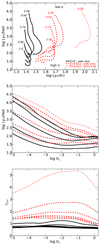 |
Fig. A.1. Impact of using a filtered ionizing continuum instead of a simple powerlaw on the observed values of Lyα/HeII, Lyα/Hβ and ηLyα. In order that the curves be aligned, the models are plotted as a function of log U* where U* = U/Fesc. In the upper panel, the U*-sequences using a filtered ionizing continuum are labelled with their respective value of Fesc. U*-sequence loci which use our default powerlaw of α = −1.5 are labelled “1.0” because the input SED is unfiltered. The dot-dashed curve (on the right of the upper panel) shows the locus of our sequence in U* that uses Fesc = 0.28, Z/Z⊙ = 0.01, α = −1.5 and the “front view”, to illustrate the combined effect of low U*, low gas metallicity, a heavily filtered ionizing continuum, and a “back-mirror”. For each combination of U* and Z/Z⊙, a lower Fesc results in a lower Lyα/HeII. |
References
- Arrigoni Battaia, F., Yang, Y., Hennawi, J. F., et al. 2015a, ApJ, 804, 26 [NASA ADS] [CrossRef] [Google Scholar]
- Arrigoni Battaia, F., Hennawi, J. F., Prochaska, J. X., & Cantalupo, S. 2015b, ApJ, 809, 163 [NASA ADS] [CrossRef] [Google Scholar]
- Asplund, M., Grevesse, N., & Jacques Sauval, A. 2006, NuPhA, 777, 1 [Google Scholar]
- Binette, L., Dopita, M. A., & Tuohy, I. R. 1985, ApJ, 297, 476 [NASA ADS] [CrossRef] [Google Scholar]
- Binette, L., Wang, J., Villar-Martin, M., Martin, P. G., & Magris, C. G. 1993a, ApJ, 414, 535 [NASA ADS] [CrossRef] [Google Scholar]
- Binette, L., Wang, J. C. L., Zuo, L., & Magris, C. G. 1993b, AJ, 105, 797 [NASA ADS] [CrossRef] [Google Scholar]
- Binette, L., Wilson, A. S., & Storchi-Bergmann, T. 1996, A&A, 312, 365 [NASA ADS] [Google Scholar]
- Binette, L., Groves, B., Villar-Martín, M., Fosbury, R. A. E., & Axon, D. J. 2003, A&A, 405, 975 [NASA ADS] [CrossRef] [EDP Sciences] [Google Scholar]
- Binette, L., Matadamas, R., Hägele, G. F., et al. 2012, A&A, 547, A29 [NASA ADS] [CrossRef] [EDP Sciences] [Google Scholar]
- Borisova, E., Cantalupo, S., Lilly, S. J., et al. 2016, ApJ, 831, 39 [NASA ADS] [CrossRef] [Google Scholar]
- Bowler, R. A. A., McLure, R. J., Dunlop, J. S., et al. 2016, MNRAS, 469, 448 [Google Scholar]
- Cantalupo, S., Arrigoni-Battaia, F., Prochaska, J. X., Hennawi, J. F., & Madau, P. 2014, Nature, 506, 63 [NASA ADS] [CrossRef] [Google Scholar]
- De Breuck, C., Röttgering, H., Miley, G., van Breugel, W., & Best, P. 2000, A&A, 362, 519 [NASA ADS] [Google Scholar]
- Dors, O. L., Agarwal, B., Hägele, G. F., et al. 2018, MNRAS, 479, 2294 [NASA ADS] [CrossRef] [Google Scholar]
- Draine, B. T., & Kreisch, C. D. 2018, ApJ, 862, 30 [NASA ADS] [CrossRef] [Google Scholar]
- Ferland, G. J., Henney, W. J., O’Dell, C. R., & Peimbert, M. 2016, Rev. Mex. Astron. Astrof., 52, 261 [NASA ADS] [Google Scholar]
- Feltre, A., Charlot, S., & Gutkin, J. 2016, MNRAS, 456, 3354 [Google Scholar]
- Ferruit, P., Binette, L., Sutherland, R. S., & Pecontal, E. 1997, A&A, 322, 73 [NASA ADS] [Google Scholar]
- Fosbury, R. A. E., Villar-Martín, M., Humphrey, A., et al. 2003, ApJ, 596, 797 [NASA ADS] [CrossRef] [Google Scholar]
- Francis, P. J. 1993, ApJ, 407, 519 [NASA ADS] [CrossRef] [Google Scholar]
- Goerdt, T., Ceverino, D., Dekel, A., & Teyssier, R. 2015, MNRAS, 454, 637 [NASA ADS] [CrossRef] [Google Scholar]
- Gould, A., & Weinberg, D. H. 1996, ApJ, 468, 462 [NASA ADS] [CrossRef] [Google Scholar]
- Haiman, Z., & Rees, M. J. 2001, ApJ, 556, 87 [NASA ADS] [CrossRef] [Google Scholar]
- Heckman, T. M., Lehnert, M. D., Miley, G. K., & van Breugel, W. 1991, ApJ, 381, 373 [NASA ADS] [CrossRef] [Google Scholar]
- Holden, B. P., Stanford, S. A., Squires, G. K., et al. 2001, AJ, 122, 629 [NASA ADS] [CrossRef] [Google Scholar]
- Humphrey, A., & Binette, L. 2014, MNRAS, 442, 753 [NASA ADS] [CrossRef] [Google Scholar]
- Humphrey, A., Villar-Martín, M., Vernet, J., et al. 2008, MNRAS, 383, 11 [NASA ADS] [CrossRef] [Google Scholar]
- Humphrey, A., Vernet, J., Villar-Martín, M., et al. 2013a, ApJ, 768, L3 [NASA ADS] [CrossRef] [Google Scholar]
- Humphrey, A., Binette, L., Villar-Martín, M., Aretxaga, I., & Papaderos, P. 2013b, MNRAS, 428, 563 [NASA ADS] [CrossRef] [Google Scholar]
- Husemann, B.,Worseck, G., Arrigoni Battaia, F., & Shanks, T. 2018, A&A, 610, L7 [NASA ADS] [CrossRef] [EDP Sciences] [Google Scholar]
- Livadiotis, G. 2018, Europhys. Lett., 122, 5 [CrossRef] [Google Scholar]
- Livadiotis, G., & McComas, D. J. 2011, ApJ, 741, 88 [NASA ADS] [CrossRef] [Google Scholar]
- McCarthy, P. J. 1993, ARA&A, 31, 639 [NASA ADS] [CrossRef] [Google Scholar]
- Nicholls, D. C., Dopita, M. A., & Sutherland, R. S. 2012, ApJ, 752, 148 [NASA ADS] [CrossRef] [Google Scholar]
- Nicholls, D. C., Dopita, M. A., Sutherland, R. S., Kewley, L. J., & Palay, E. 2013, ApJS, 207, 21 [NASA ADS] [CrossRef] [Google Scholar]
- Prochaska, J. X., Hennawi, J. F., & Simcoe, R. A. 2013, ApJ, 762, L19 [NASA ADS] [CrossRef] [Google Scholar]
- Robinson, A., Binette, L., Fosbury, R. A. E., & Tadhunter, C. N. 1987, MNRAS, 227, 97 [NASA ADS] [CrossRef] [Google Scholar]
- Rosdahl, J., & Blaizot, J. 2012, MNRAS, 423, 344 [NASA ADS] [CrossRef] [Google Scholar]
- Schaerer, D. 2002, A&A, 382, 28 [NASA ADS] [CrossRef] [EDP Sciences] [Google Scholar]
- Shibuya, T., Ouchi, M., Konno, A., et al. 2018, PASJ, 70, S14 [Google Scholar]
- Shull, J. M., Stevans, M., & Danforth, C. W. 2012, ApJ, 752, 162 [NASA ADS] [CrossRef] [Google Scholar]
- Sobral, D., Matthee, J., Darvish, B., et al. 2015, ApJ, 808, 139 [NASA ADS] [CrossRef] [Google Scholar]
- Sobral, D., Matthee, J., Darvish, B., et al. 2018, MNRAS, 477, 2817 [NASA ADS] [CrossRef] [Google Scholar]
- Sobral, D., Matthee, J., Brammer, G., et al. 2019, MNRAS, 482, 2422 [NASA ADS] [CrossRef] [Google Scholar]
- Stevans, M. L., Shull, J. M., Danforth, C. W., & Tilton, E. M. 2014, ApJ, 794, 75 [NASA ADS] [CrossRef] [Google Scholar]
- Taniguchi, Y., Trentham, N., Ikeuchi, S., et al. 2001, ApJ, 559, L9 [NASA ADS] [CrossRef] [Google Scholar]
- Telfer, R. C., Zheng, W., Kriss, G. A., & Davidsen, A. F. 2002, ApJ, 565, 773 [NASA ADS] [CrossRef] [Google Scholar]
- Tenorio-Tagle, G., Silich, S. A., Kunth, D., Terlevich, E., & Terlevich, R. 1999, MNRAS, 309, 332 [NASA ADS] [CrossRef] [Google Scholar]
- van Ojik, R., Rottgering, H. J. A., Miley, G. K., et al. 1994, A&A, 289, 54 [NASA ADS] [Google Scholar]
- Vasyliunas, V. M. 1968, ASSL, 10, 622 [NASA ADS] [CrossRef] [Google Scholar]
- Vernet, J., Fosbury, R. A. E., Villar-Martín, M., et al. 2001, A&A, 366, 7 [NASA ADS] [CrossRef] [EDP Sciences] [Google Scholar]
- Vernet, J., Lehnert, M. D., De Breuck, C., et al. 2017, A&A, 602, L6 [NASA ADS] [CrossRef] [EDP Sciences] [Google Scholar]
- Villar-Martín, M., Binette, L., & Fosbury, R. A. E. 1996, A&A, 312, 751 [NASA ADS] [Google Scholar]
- Villar-Martín, M., Tadhunter, C., & Clark, N. 1997, A&A, 323, 21 [NASA ADS] [Google Scholar]
- Villar-Martín, M., Vernet, J., di Serego Alighieri, S., et al. 2003, MNRAS, 346, 273 [NASA ADS] [CrossRef] [Google Scholar]
- Villar-Martín, M., Cerviño, M., & González Delgado, R. M. 2004, MNRAS, 355, 1132 [NASA ADS] [CrossRef] [Google Scholar]
- Villar-Martín, M., Humphrey, A., De Breuck, C., et al. 2007, MNRAS, 375, 1299 [NASA ADS] [CrossRef] [Google Scholar]
All Tables
Illustrating the impact of low gas metallicity and/or a filtered ionizing SED on the production of Lyα.
All Figures
|
Fig. 1. Filtered AGN spectral energy distributions described in Sect. 3.8. These correspond to escape fractions of 0.28 (solid black line), 0.50 (solid red line), 0.74 (solid blue line) and 0.90 (solid cyan line). For comparison, we also show the emergent distribution from a typical ionization-bounded model (dashed black line): the UV part of the spectrum has been completely absorbed, while some X-rays still escape through the cloud. The vertical axis (normalized flux density or Sν) gives the power per unit area per unit frequency in arbitrary units. The escape fractions are in photon number flux, while the SEDs are plotted in energy flux per unit frequency (Sν). |
| In the text | |
|
Fig. 2. Selected sequences in U plotted for Lyα/HeII vs. Lyα/Hβ, Lyα/Hα, Hα/Hβ, or [OIII] λ5007/Hβ. Each sequence represents a progression in U, for each of the three values of Z. Also shown are sequences in U using κ = 20 for Z/Z⊙ = 0.01 and 1.0 (dotted curves). All models in this figure use power index α = −1.5. The lower two panels show Lyα/HeII vs. U (left) and the ratio of Lyα photons to ionizing photons (ηLyα; right) for the same model sequences. The model loci cover the range of ionization parameter −5 < log U < 0.25. |
| In the text | |
|
Fig. 3. Impact of the powerlaw index of the ionizing spectrum on Lyα/HeII, Lyα/Hβ and ηLyα. The model loci cover the range of ionization parameter −5 < log U < 0.25. |
| In the text | |
|
Fig. 4. Impact of viewing angle on the observed Lyα/HeII, Lyα/Hβ and ηLyα values. The green curve shows the locus of our sequence in U using Z/Z⊙ = 0.01, α = −2.0 and the “front view”, to illustrate the combined effect of low U, low gas metallicity, a relatively soft ionizing continuum, and a “back-mirror”. The model loci cover the range of ionization parameter −5 < log U < 0.25. |
| In the text | |
|
Fig. 5. Impact of using a filtered ionizing continuum instead of a simple powerlaw on the observed values of Lyα/HeII, Lyα/Hβ and ηLyα. U-sequences using a filtered ionizing continuum are labelled with their value of Fesc. U-sequence loci which use our default powerlaw of α = −1.5 are labelled “1.0” because the input SED is unfiltered. The dot-dashed curve (on the right of the upper panel) shows the locus of our sequence in U that uses Fesc = 0.28, Z/Z⊙ = 0.01, α = −1.5 and the “front view”, to illustrate the combined effect of low U, low gas metallicity, a heavily filtered ionizing continuum, and a “back-mirror”. For each combination of U and Z/Z⊙, a lower Fesc results in lower Lyα/HeII and higher ηLyα. In Fig. A.1 we show an alternate version of this Figure, plotted with U scaled by 1/Fesc to aid comparison with our other models. |
| In the text | |
|
Fig. 6. Impact of gas density on the observed Lyα/HeII, Lyα/Hβ and ηLyα values. The model loci cover the range of ionization parameter −5 < log U < 0.25. |
| In the text | |
|
Fig. 7. Diagnostic diagrams comparing Pop III (heavy orange line) and several AGN photoionization models. The AGN model U-sequences shown here are: α = −1.5 (thick black line); α = −2.0 (thin black line); α = −1.5 with “front view” (“back-mirror”) (dot-dashed line); photoionization by our Fesc filtered AGN continuum (dashed line). All models shown in this figure use Z/Z⊙ = 0.01. See main text for further details. The model loci cover the full range of ionization parameter in our model grid, i.e., −5.55 < log U < 0.25. |
| In the text | |
|
Fig. 8. Lyα/HeII vs. Lyα/CIV showing the locus of several of our photoionization model sequences, along with the measurements or 3σ lower limits on these ratios taken from the Lyα halos of z ∼ 3.5 quasars of Borisova et al. (2016). The model loci cover the full range of ionization parameter in our model grid, i.e., −5 < log U < 0.25. The horizontal green dotted line marks the boundary between what we define as “extreme” and “normal” Lyα/HeII flux ratios. |
| In the text | |
|
Fig. A.1. Impact of using a filtered ionizing continuum instead of a simple powerlaw on the observed values of Lyα/HeII, Lyα/Hβ and ηLyα. In order that the curves be aligned, the models are plotted as a function of log U* where U* = U/Fesc. In the upper panel, the U*-sequences using a filtered ionizing continuum are labelled with their respective value of Fesc. U*-sequence loci which use our default powerlaw of α = −1.5 are labelled “1.0” because the input SED is unfiltered. The dot-dashed curve (on the right of the upper panel) shows the locus of our sequence in U* that uses Fesc = 0.28, Z/Z⊙ = 0.01, α = −1.5 and the “front view”, to illustrate the combined effect of low U*, low gas metallicity, a heavily filtered ionizing continuum, and a “back-mirror”. For each combination of U* and Z/Z⊙, a lower Fesc results in a lower Lyα/HeII. |
| In the text | |
Current usage metrics show cumulative count of Article Views (full-text article views including HTML views, PDF and ePub downloads, according to the available data) and Abstracts Views on Vision4Press platform.
Data correspond to usage on the plateform after 2015. The current usage metrics is available 48-96 hours after online publication and is updated daily on week days.
Initial download of the metrics may take a while.