| Issue |
A&A
Volume 620, December 2018
|
|
|---|---|---|
| Article Number | A145 | |
| Number of page(s) | 16 | |
| Section | Stellar structure and evolution | |
| DOI | https://doi.org/10.1051/0004-6361/201834161 | |
| Published online | 11 December 2018 | |
Short-term variability and mass loss in Be stars
IV. Two groups of closely spaced, approximately equidistant frequencies in three decades of space photometry of ν Puppis (B7-8 IIIe)⋆,⋆⋆,⋆⋆⋆
1
European Organisation for Astronomical Research in the Southern Hemisphere (ESO), Karl-Schwarzschild-Str. 2, 85748, Garching
e-mail: This email address is being protected from spambots. You need JavaScript enabled to view it.
2
Astronomical Institute, Wrocław University, Kopernika 11, Wrocław 51-622, Poland
3
European Organisation for Astronomical Research in the Southern Hemisphere (ESO), Santiago 19, Casilla 19001, Chile
4
Center for High Angular Resolution Astronomy and Department of Physics and Astronomy, Georgia State University, GA 30302-5060, Atlanta PO Box 5060, USA
5
Nicolaus Copernicus Astronomical Center, ul. Bartycka 18, Warsaw 00-716, Poland
6
Observatório Nacional, Rua General José Cristino 77, São Cristóvão, Rio de Janeiro 20921-400, Brazil
7
Instituto de Astronomia, Geofísica e Ciências Atmosféricas, Universidade de São Paulo, Cidade Universitária, Rua do Matão 1226, São Paulo, SP 05508-900, Brazil
8
Institut für Kommunikationsnetze und Satellitenkommunikation, Technical University Graz, Inffeldgasse 12, Graz 8010, Austria
9
Département de physique and Centre de Recherche en Astrophysique du Québec (CRAQ), Université de Montréal, CP 6128, Succ. Centre-Ville, Montréal Québec H3C 3J7, Canada
10
AAVSO Headquarters, 49 Bay State Rd., Cambridge, MA 02138, USA
11
Department of Astronomy and Astrophysics, University of Toronto, 50 St. George St., Toronto, Ontario M5S 3H4, Canada
12
Department of Physics and Space Science, Royal Military College of Canada, Stn Forces, Ontario K7K 7B4, , Kingston PO Box 17000, Canada
13
Institute of Astrophysics, University of Vienna, Universitätsring 1, Vienna 1010, Austria
14
Universität Innsbruck, Institut für Astro- und Teilchenphysik, Technikerstrasse 25, Innsbruck 6020, Austria
Received:
30
August
2018
Accepted:
13
October
2018
Abstract
Context. In early-type Be stars, groups of nonradial pulsation (NRP) modes with numerically related frequencies may be instrumental for the release of excess angular momentum through mass-ejection events. Difference and sum/harmonic frequencies often form additional groups.
Aims. The purpose of this study is to find out whether a similar frequency pattern occurs in the cooler third-magnitude B7-8 IIIe shell star ν Pup.
Methods. Time-series analyses were performed of space photometry with BRITE-Constellation (2015, 2016/17, and 2017/18), SMEI (2003–2011), and HIPPARCOS (1989–1993). Two IUE SWP and 27 optical echelle spectra spanning 20 years were retrieved from various archives.
Results. The optical spectra exhibit no anomalies or well-defined variabilities. A magnetic field was not detected. All three photometry satellites recorded variability near 0.656 c/d which is resolved into three features separated by ∼0.0021 c/d. Their first harmonics and two combination frequencies form a second group, whose features are similarly spaced by 0.0021 c/d. The frequency spacing is very nearly but not exactly equidistant. Variability near 0.0021 c/d was not detected. The long-term frequency stability could be used to derive meaningful constraints on the properties of a putative companion star. The IUE spectra do not reveal the presence of a hot subluminous secondary.
Conclusions. ν Pup is another Be star exhibiting an NRP variability pattern with long-term constancy and underlining the importance of combination frequencies and frequency groups. This star is a good target for efforts to identify an effectively single Be star.
Key words: asteroseismology / stars: emission-line, Be / stars: mass-loss / techniques: photometric / stars: rotation
Based in part on data collected by the BRITE-Constellation satellite mission, built, launched and operated thanks to support from the Austrian Aeronautics and Space Agency and the University of Vienna, the Canadian Space Agency (CSA), and the Foundation for Polish Science & Technology (FNiTP MNiSW) and National Science Centre (NCN).
Based in part on observations made with ESO Telescopes at the La Silla Paranal Observatory under programme ID 074.D-0240.
Light curve data are only available at the CDS via anonymous ftp to cdsarc.u-strasbg.fr (130.79.128.5) or via http://cdsarc.u-strasbg.fr/viz-bin/qcat?J/A+A/620/A145
© ESO 2018
1. Introduction
When a rapidly rotating massive star evolves, it may have to solve a problem when angular momentum is transported from the contracting core to the outer layers (Krtička et al. 2011; Granada et al. 2013). Apart from mixing, nonradial g-modes may be involved in the angular-momentum transport process (Neiner et al. 2013, and references therein). These stars may appear as Be stars which are unique in that only Be stars seem to possess circumstellar disks built from self-ejected matter (Rivinius et al. 2013). In these little to moderately evolved stars, radiative winds do not produce major mass-loss rates (Krtička 2014). Broad consensus exists that the near-critical rotation (Frémat et al. 2005; Meilland et al. 2012; Rivinius et al. 2013) is a necessary condition for the mass loss. Numerous observational studies (Rivinius et al. 1998, 2013; Huat et al. 2009; Baade et al. 2017, 2018a) suggest that much of the star-to-disk mass-transfer process takes place in discrete events, which cover a wide range in cadence and amplitude (Semaan et al. 2018; Bernhard et al. 2018). Although having the appearance of mass-loss events, they may actually be more accurately described as angular-momentum-loss events. Angularmomentum- loss rates were recently measured for a large sample of Be stars (Rímulo et al. 2018).
Evidence is mounting, broadly supporting the hypothesis (Rivinius et al. 1998; Baade et al. 2018b) that multi-mode nonradial pulsation (NRP) plays a central role in the conditioning of the stellar atmosphere for outbursts. Which specific conditions do lead to an outburst is entirely unknown except that temporarily much increased NRP amplitudes can have triggering power. Interacting NRP modes may operate the valves of the angularmomentum- loss process. Baade et al. (2018b) have presented a scheme of nested clocks with hierarchically decreasing frequencies, which all derive from stellar pulsation frequencies and govern the opening and closing of the angular-momentum-loss valves. More-massive stars may have to open these valves more often and/or more widely because they evolve more rapidly. This mass-dependence of the activity seems confirmed by the long-term photometry of large numbers of Be stars with a wide range of spectral subclasses (e.g., Hubert & Floquet 1998; Bernhard et al. 2018). Brightenings indicate ejections of gas, which reprocesses the stellar light; in edge/equator-on systems such events lead to fadings when the disk attenuates the stellar light (Haubois et al. 2014).
Overview of the BRITE, HIPPARCOS, and SMEI observations.
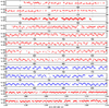 |
Fig. 1. All main strings of BRITE observations of ν Pup in 2015, 2017, and 2018. Very long segments are split with partial duplications. The ordinate is in units of instrumental magnitudes with arbitrary zero point. Symbols: red +: BHr2015; red °: BHr2017; red ×: BTr2017; blue +: BLb2017; red □: BHr2018. Intercomparison of observations in identical time intervals but from different satellites shows that the most regular segments of the light curves are representative and the others deviate as a result of noise. The amplitude was largest in 2017 and lowest in 2018. In the bottom panel, between days 1145 and 1150 and shortly before day 1160, there may have been some mini outbursts. |
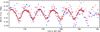 |
Fig. 2. A 10-d stretch (in 2017) of observations of ν Pup with BRITE satellites BLb (blue filled triangles), BHr (red asterisks), and BTr (red crosses). The zeropoints of the magnitude scale are arbitrary. Black dots represent a sine fit to the BHr data. The deviation from sinusoidality is most clearly seen in the BHr data. |
At the cool limit of the so-called Be phenomenon, spectroscopic evidence of a disk is often restricted to shell absorption lines. However, recent observations by Shokry et al. (2018) have demonstrated that, with the help of high-quality spectral line profiles, weak Hα emission can be detected in many more late B-type stars than previously thought. The variability of their emission lines seems to be much slower and reach lower amplitudes than displayed by many early-type Be stars (Barnsley & Steele 2013). Photospheric line-profile variability is also much less pronounced in late-type Be stars (Baade 1989b).
With the advent of powerful space photometers, a substantially more detailed view of the variability of late-type Be stars is emerging. Recently, Kepler observations of KIC 11971405 (HD 186657; B5 IV-Ve; Pápics et al. 2017) have revealed one of the most intricate networks of NRPs known in Be stars. Most variabilities have sub-mmag amplitudes. At B5, HD 186567 is also one of the cooler Be stars with detected NRPs. Still cooler is β CMi at B8, for which MOST recorded many NRP modes with similarly low amplitudes (Saio et al. 2007). In observations of the B7 V star CoRoT 101486436, Semaan et al. (2018) find this star’s variability to resemble that of β CMi; however, the peak-to-valley amplitude of a 0.03 c/d beat (perhaps: difference) frequency has an amplitude of 12 000 ppm with individual frequencies near 5 c/d reaching up to 3000 ppm.
During the monitoring period with Kepler, also KIC 11971405 underwent some small outbursts. As Baade et al. (2018b) showed, the spacing in time of some of these events can be related to difference frequencies of some NRP modes with the highest amplitudes. Such coupling had previously been found in BRITE, Kepler, and CoRoT observations of several early-type Be stars (Baade et al. 2016, 2018b; Rivinius et al. 2016, and in prep.). White et al. (2017) conclude that Kepler/K2 observations of four Be stars in the Pleiades are consistent with this hypothesis for the two least evolved Be stars, Merope (B6 IVe) and Pleione (B8 Vne).
Late-B spectral types are also the realm of the historically mythical Maia variables. Maia itself (20 Tau, B7 III) was finally shown not to be pulsating but exhibiting slow rotational modulation (White et al. 2017). However, there do exist probable g-mode pulsators between the conventional Slowly Pulsating B Star (SPB) and γ Dor domains (e.g. Mowlavi et al. 2013); this includes late B-type stars. Whether the pulsations of the other six B stars in the Pleiades studied by White et al. (2017) fall into just one single category is unknown. The light curves of Alcyone (B7 IIIe), Electra (B6 IIIe), Merope (B6 IVe), and Pleione (B8 Vne) exhibit clear variations of their upper and lower envelopes which may be due to the beating of a few single frequencies. A similar pattern is absent in the normal binary B star Atlas (B8 III + B8 V) and much less prominent in the other normal B-type star Taygeta (B6 IV) if present at all. White et al. (2017) explicitly report frequency groups for the Be stars Alcyone, Electra, and Taygeta and describe the variability of Merope (Be) and Taygeta (B) in terms of closely spaced frequencies, which is consistent with the presence of frequency groups.
Frequency groups are characteristic of Be stars (Balona et al. 2011; Baade et al. 2017; Semaan et al. 2018) but do not seem limited to them (Kurtz et al. 2015), and not all pulsating Be stars display frequency groups. The latter authors proposed that frequency groups may be understood as clusters of combination frequencies of NRP modes. This was confirmed by Pápics et al. (2017) in the same data. In the early-type Be star 25 Ori, (Baade et al. 2018b, an extended version of this work with additional BRITE and revised SMEI observations is in preparation) tentatively identified an extremely rich pattern of grouped combination frequencies.
It is proposed (Cameron et al. 2008; Rivinius et al. 2016; White et al. 2017) that Be stars may be rapidly rotating SPB stars. However, among the B-type stars without Be characteristics, neither SPB stars nor any other type of pulsating star span such a wide range in effective temperature as the Be stars do. On the other hand, pulsations of Be stars do not seem to significantly extend to lower or higher temperatures than those of other pulsating OB stars do, and the combined role of rapid rotation and mass and angular-momentum leakage is still to be explored in detail.
The third-magnitude late-type Be star ν Pup (HR 2451, HIP 31685, HD 47670) has not been given much attention by spectroscopists. Wright (1909) described Hγ as consisting of a broad absorption with superimposed fairly sharp central absorption. Such shell components occur in Be stars if the star is viewed equator-on and the line of sight passes through the disk. In eight spectra, the radial velocity of the narrow component varied from +33 km s−1 in 1904 to +20 km s−1 in 1908. Temporary shell absorption flanked by weak line emission in Hα is also detected by Rivinius et al. (1999, 2006). Shell absorptions were not reported by Pickering & Cannon (1897) and by Slettebak et al. (1975) so that the disk is probably not persistent.
Cousins (1987) treated ν Pup as a secondary photometric standard. On the other hand, from HIPPARCOS observations, Koen & Eyer (2002) reported a variability with frequency 0.15292 c/d and amplitude 0.00117 mag. At other wavelengths, ν Pup has remained inconspicuous: It was not detected in the ROSAT All Sky X-ray Survey (Berghoefer et al. 1996), and Bodensteiner et al. (2018) did not find it embedded in a mid-IR nebulosity. Eggleton & Tokovinin (2008) do not list ν Pup as multiple.
ν Pup was selected from the Be stars observed with BRITE-Constellation because of its relatively low temperature (extending earlier studies with BRITE of hotter Be stars), its brightness (yielding a better signal-to-noise ratio with BRITE), and the unusual simplicity, at a first glance, of its frequency spectrum.
2. Observations
New observations were obtained with the BRITE-Constellation of nanosatellites. Its mission and operations concepts were described by Weiss et al. (2014), who also provide the definition of the BRITE-Constellation photometric passbands, and Pablo et al. (2016), respectively. A total of three of the five cubesats were employed for different time intervals in 2015 (BRITE field 08-VelPic-I-2015), 2016/17 (BRITE field 23-VelPic-II-2016), and 2017/18 (BRITE field 33-VelPic-III-2017) as detailed in Table 1, which also contains the number of raw observations and derived data points. The BRITE data are available from the BRITE photometry wiki1. For simplicity, the three datasets are referred to below as B2015, B2017, and B2018, respectively. The rationale for additional processing of the pipeline-reduced data (Popowicz et al. 2017) was explained in much detail by Pigulski et al. (2018) and Pigulski (2018). For the observations of ν Pup, it was implemented and applied as described in Baade et al. (2018a).
Pipeline-reduced BRITE datasets are subdivided into so-called setups if some observing condition changed during the observing season. The most common reason is re-acquisition of the field. For all three satellites, temperature jumps occurred within some setups, and the correlations with CCD temperature of magnitudes before and after such events were different. Therefore such setups were split, and the decorrelation was performed separately for each data segment. An overview of all major segments of BRITE observations can be gained from Fig. 1. Figure 2 presents a ten-day interval at higher resolution with observations from BLb, BHr, and BTr in 2017.
Archival observations (Jackson 2018, priv. comm.) with the Solar Mass Ejection Imager (SMEI; Jackson et al. 2004) extend from Feb. 2, 2003 through Sept. 28, 2011. Contrary to an earlier study in this series using SMEI data (Baade et al. 2018a, who also describe SMEI from the stellar-photometry point of view), the data now available identify with which of the three cameras a given measurement was made. This vastly improves the scope of the preparation of the data for time series analysis.
SMEI photometry exhibits large-amplitude annual variations the details of which are strongly dependent on position in the sky because the objective of SMEI was to observe light scattered by electrons ejected by the Sun. For ν Pup, these artifacts were much reduced in a multi-step procedure applied separately to the data from each camera. First, for each data point its difference from a sliding average over ten days was calculated in units of flux as well as of the standard deviation in the ten-day bin concerned. In a diagram with these two parameters, several narrow rays can be seen fanning out from the origin. Outliers were clipped in both coordinates. Second, a second-order polynomial was fitted to the light curve and subtracted, and newly apparent outliers were eliminated. In the third step, annual and half-annual variations were removed by subtracting fitted sine functions. After folding the data with a period of one year, new outliers were identified by eye (because of their strongly non-Gaussian distribution) and removed. These latter two steps were repeated for frequencies between 0.02 and 0.06 c/d, which may be (partly) related to the Moon. In the sixth step, the very pronounced 1-c/d variability was subtracted, and, finally, remaining data points with large values of SMEI parameter sigPSF were also removed. Thereafter, the three datasets were merged for the subsequent time-series analysis. All together, these seven steps reduced the numbers of data points from the initial 7127/18516/12974 for Cameras 1/2/3 to the final 5353/16380/9974, respectively.
A further archival dataset is available from HIPPARCOS (ESA 1997). It consists of 115 photometric measurements obtained between Nov. 30, 1989 and March 5, 1993. There are variations on timescales of several hundred days, and several of them fold the data to well-behaved light curves. They were not removed because none of them stands out above the others. The dataset contains only one apparent outlier, which was retained.
The time-series analysis (TSA) of the BRITE, SMEI, and HIPPARCOS data was performed with implementations of Scargle’s method (Scargle 1982) and plain power-spectrum calculation in the TSA package of MIDAS (Banse 2003). The differences between the methods seem negligible. With orbital periods near 100 min, both BRITE and SMEI have Nyquist frequencies around 7 c/d. The final power spectra between 0.4 c/d and 1.5 c/d for SMEI and all BRITE data are compiled in Fig. 3.
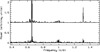 |
Fig. 3. Power spectra of BRITE (vertically offset for clarity; all datasets combined) and SMEI (bottom) photometry. Two frequency groups near 0.656 c/d and 1.31 c/d as well as 1-c/d variability are present. The power spectra were scaled to the same peak strength of the 0.656-c/d groups. |
Pipeline-reduced spectra were downloaded from the HEROS2, the ESO3 (for FEROS), the CFHT4 (for ESPaDOns), and MAST5 (for IUE) online archives. HEROS (Kaufer 1998), FEROS (Stahl et al. 1999), and ESPaDOns (Donati et al. 2006) are optical echelle spectrographs with approximate resolving powers of 20 000, 48 000, and 68 000, respectively. With HEROS and FEROS only single spectra per night were obtained every couple of days or weeks (they include the spectra used by Rivinius et al. 2006). By contrast, all 40 ESPaDOns spectra were secured within about one hour. A description of the International Ultraviolet Explorer (IUE) is available from Boggess et al. (1978).
3. Analysis
This section is structured as follows: Sect. 3.1 describes the appearance of the spectra; a simple stellar model is provided, radial velocities are measured and analyzed for periodic variations, and limits are placed on the UV flux contributed by a subluminous hot companion. A general overview of the photometric variability is given in Sect. 3.2. It is followed by the description of the two frequency groups found (Sect. 3.3.1) and their simulation (Sect. 3.3.2). The final subsections deal with mass loss (Sect. 3.4) and, from photometric Doppler shifts, derive limits on the mass and orbital period of a putative companion (Sect. 3.5).
3.1. Spectroscopy
In the ESPaDOnS spectra, the strengths of HeI 4471 and MgII 4481 are indistinguishable. In the classification scheme of Lesh (1968), this corresponds to spectral type B8 on the main sequence. Pickering & Cannon (1897) and Slettebak et al. (1975) classified ν Pup as B8. However, the weakly developed wings of the Balmer lines indicate luminosity class III-IV for which case Lesh (1968) notes that the He lines are weaker than on the main sequence. This suggests an MK type closer to B7 III. For B7 III and B8 III, the grid of stellar parameters calculated by Shokry et al. (2018), which is based on Zorec et al. (2009), is provided in Table 2. The derived parameter values are comparable to those compiled by White et al. (2017) for the B-type stars in the Pleiades. However, the calculated v sin i of 170 km s−1 is not a good match to the observations which are in much better agreement with the value of 246 km s−1 listed by Royer et al. (2002). In the following, averages of the two parameter sets are adopted.
Because of the high apparent brightness (v = 3.17 mag, Ducati 2002) and late spectral subtype of ν Pup, the star has a relatively large parallax. The revised HIPPARCOS measurement of 8.78 mas (van Leeuwen 2007), which was suggested to replace the original value of 7.71 mas (Perryman et al. 1997), is in excellent agreement with the Gaia DR2 value of 8.9182 mas (Gaia Collaboration 2018). However, for both projects, stars as bright as ν Pup are a challenge. With 0.75 mag as the bolometric correction and 0.05 mag for the visual interstellar extinction, the averaged parallax of 8.85 mas implies a bolometric magnitude of −2.9 mag, 0.26 mag brighter than the average of the two models (Table 2). The difference is not significant; however, if it is attributed entirely to the radius estimate (for a uniform stellar disk), the radius derived from the observations is 12% larger than the calculated one.
Stellar parameters calculated for spectral types B7 III and B8 III as described in Shokry et al. (2018).
For the time spanned by the spectra, the evolution of the Hα line is documented in Table 3. A very weakly developed circumstellar disk was directly detected only between 1995 and 1999. However, the presence of strong central quasi-emission features in MgII 4481 in 1985 (Baade 1989a) suggests (Rivinius et al. 1999) that the disk may have been much denser a decade before. Considering the general slow variability of disks around late-type Be stars, perhaps the 1995–1999 observations trace only the terminal phase of the disk dissipation.
Appearance of the Hα line in ν Pup at various times.
Means of radial velocities of stellar Balmer lines Hγ, Hδ, Hϵ, and H8, of the shell absorption in Hα, and of other stellar lines (He I 4026, He I 4143, He I 4471, and Mg II 4481).
All stronger non-Balmer lines were very carefully scrutinized for line-profile variations. However, because the depth of the lines is only about 5% of the adjacent continuum level, non-Gaussian pixel noise and instrumental variations in the continuum shape make this search exceedingly difficult. The width of the best isolated of these lines, HeI 4026, measured as the full width at half maximum of a fitted Gaussian, was constant to ±4.1% in the HEROS and to ±2.5% in the FEROS spectra. This scatter is plausibly explained by the said imperfections of the spectra. The variability is stronger in the line wings. In some of the best defined line profiles, the wings assume the shape of a ramp on either the blue or the red side, while the respective other wing is much steeper. This can be the signature of nonradial pulsation (Rivinius et al. 2003). Phasing of selected line profiles with the main photometric frequency near 0.656 c/d (cf. Sect. 3.2) did not bring out a clearly coherent pattern because instrumental properties dominated. No obvious variations were seen in the strength of any line, in agreement with earlier observations by Baade (1989a), who obtained two pairs of high-resolution, high-signal-to-noise ratio profiles of He I 4471 and Mg II 4481 in two consecutive nights.
Radial velocities (RVs) were measured in the Hβ-H12 Balmer, several He I, and some metal lines. The results are given in Table 4 and Fig. 4 separately for (i) the Hγ-H8 Balmer lines (which are unaffected by circumstellar components), (ii) HeI λλ 4026, 4143, and 4471 as well as MgII 4481 and, when possible, for the shell absorption component in Hα. The measurements in the Balmer lines are probably compromised by the residual echelle ripple in the pipeline-reduced spectra. The radial velocities of the other stellar lines suffer from this, too, but mainly from pixel noise; there may also be an effect of the suspected line-profile variability. The homogeneity of the shell velocities is reduced by variable telluric absorption features.
Because the extremely uneven distribution of epochs of the RV measurements (Table 4, Fig. 4) prevents the direct determination of a putative orbital period, the full parameter space was explored to find out where any permissible orbits might occur. Frequencies and RV amplitudes were derived simultaneously from sine fits to the non-Balmer RVs in Table 4 with 250 000 equally spaced start frequencies from 0.000004 to 1 c/d. This sampling was chosen to match the time span of the spectra of 11 300 d (Table 4). The mean amplitude is 2.95 ± 1.3 km s−1 with a maximum of 8.5 km s−1 so that any real circular orbital amplitude should not exceed 10 km s−1. In Fig. 5, the results are mapped onto the frequency–amplitude plane binned to pixels of 0.008 c/d and 0.1 km s−1, respectively. On average, the number of frequency-and-amplitude pairs per such bin is ten. However, the number of amplitudes above 4 km s−1 is very small so that 30 ± 6 pairs per pixel is a more realistic estimate of the floor value. The peaks in Fig. 5 reaching levels of 250 pairs are formally highly significant. However, in a genuine binary system, only one such pixel can represent the correct frequency and amplitude. Since no peak stands out above the others, they only permit an upper limit to be placed on the amplitude of a putative binary. Inspection of Fig. 5 supports the validity of the above value of 10 km s−1. By contrast, the possible period is not usefully constrained by the RVs.
The ESPaDOnS observations form part of the BRITE spectropolarimetry programme which targeted 573 stars brighter than V = 4 mag to search for magnetic fields (Neiner et al. 2017). In agreement with similar observations of 85 classical Be stars (Wade et al. 2016), no large-scale field was found (Wade, priv. comm.; Neiner et al., in prep.).
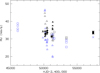 |
Fig. 4. Radial velocities of stellar Hδ-H8 lines (open black symbols), other stellar lines (He I 4026.2, He I 4143.8, He I 4471.5, and Mg II 4481.2; open blue symbols), and the circumstellar shell line in Hα (filled symbols). It can be seen that the accuracy of the ESPaDOnS measurements (crosses near mJD 57500) is highest, that of the HEROS measurements (triangles) lowest. Measurements with FEROS (CES) are plotted as squares (circles). See also Table 4 and Sect. 3.1. |
The star ν Pup lies in the temperature range of various types of chemically peculiar stars. Therefore, the co-added ESPaDOnS spectrum was inspected for traces of anomalous abundances. No lines were found from HgII (3984 Å), MnII (4137 Å; the lines between 3442 Å and 3498 Å are outside the [useful] range of all three spectrographs), CrII (4559 Å), SrII (4078, 4215, and 4305 Å), and EuII (4205 Å); however, only spectral synthesis could establish quantitative limits. SiII λλ4128,4131, λλ5041,5056, and λλ 6347,6371 are present at normal strength and, in the other spectra, exhibit no variability.
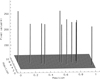 |
Fig. 5. Plane with coordinates of frequency (in c/d, abscissa) and radial-velocity amplitude (in km s−1, ordinate). The data axis provides the number of frequency–amplitude data pairs resulting from circular orbits fitted to the radial velocities in Table 4, as described in Sect. 3.1. Each spike has a footprint of dimensions 0.008 c/d and 0.1 km s−1; only for better visibility were they enlarged. The floor level is ≤30 ± 6 data points per pixel. |
The two IUE SWP high-dispersion spectra from 1988 April were processed as described in Wang et al. (2017). Owing to the low distance to ν Pup, interstellar lines did not have to be removed. The search for an ultraviolet signature of a hot companion used the cross-correlation technique successfully employed by Wang et al. (2018). Tlusty (Lanz & Hubeny 2003) template spectra for temperatures of 27.5, 35, and 45 kK were employed.
3.2. Photometry: overview
The point-spread function of SMEI has a diameter of order one degree (Hick et al. 2007), and BRITE uses apertures of up to 25 arcmin (Popowicz et al. 2017). Within 30 arcmin from ν Pup, SIMBAD (Wenger et al. 2000) lists 93 objects the variability of which may contaminate measurements of ν Pup. The brightest sources by far are the two B3 V stars HIP 31642 (V = 6.86 mag) and HIP 31875 (V = 7.41 mag) at distances of 16 and 25 arcmin, respectively. All other sources with known brightness are of ninth magnitude or fainter, therefore each contributing (mostly: much) less than 1% to the total flux. The scatter of the HIPPARCOS magnitudes of HIP 31642 (HIP 31875) is 7.7 (9.8) mmag. Fitted sine curves with frequency f2 = 0.655802 c/d reported below have semi-amplitudes of 2.2 and 1.3 mmag for HIP 31642 and HIP 31875, respectively. Therefore, any corruption by these two stars of the variabilities observed in ν Pup is negligible.
The BRITE and SMEI observations are highly complementary. The former have a much higher fidelity per data point and reveal details of the light curve while the SMEI data extend over a much longer continuous time span and are better suited to study long-term variations and resolve closely spaced features in the power spectrum as has been shown in a number of independent analyses (e.g., Goss et al. 2011; Howarth & Stevens 2014; Baade et al. 2018a). The noise and the time span of the HIPPARCOS data are intermediate between those of SMEI and BRITE whereas the number of HIPPARCOS data points is one to two orders of magnitude smaller. Accordingly, the HIPPARCOS photometry can be used to trace back, over more than a decade, major findings made with the other satellites.
Simple inspection of the non-phase-folded BRITE light curve (Fig. 1) seems to suggest that it is single-periodic, not sinusoidal, and, on timescales of months or years, strongly variable in amplitude. There are indications that consecutive light cycles do not repeat perfectly (Fig. 2). Compared to other Be stars, the BRITE power spectrum of ν Pup (Fig. 3) also looks unusually simple with only one very dominating feature near 0.656 c/d. However, the sensitivity of MOST, Kepler, and CoRoT to variabilities of B-type stars (cf. Introduction) was at least two orders of magnitude better than that of BRITE, which did not reach sub-mmag levels for ν Pup. Moreover, the simplicity may be just apparent because time-series analyses of different segments of the BRITE photometry return very substantially different frequencies. According to Fig. 2, there is no appreciable phase difference between the variabilities in the blue and the red BRITE passbands so that combining all BRITE data is not expected to introduce artifacts into the power spectra.
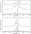 |
Fig. 6. Upper panel: power spectra of HIPPARCOS (top), BRITE (middle) and SMEI (bottom, with frequencies c1–c6 (Table 5) appearing between 1.3075 and 1.32 c/d) observations. The three peaks in the SMEI power spectrum correspond with frequencies f1–f3 (Table 5). Lower panel: SMEI (bottom) and BRITE (top) power spectra of the frequency group near 1.31 c/d. The frequency range is stretched by a factor of 2 w.r.t. the upper panel so that base frequencies and harmonics line up. The power scales are arbitrary and cannot be compared between the satellites. The SMEI power scales for the two frequency groups differ by about a factor of 20. |
At low resolution, the SMEI power spectrum reveals the same overall structure as that obtained with BRITE (Fig. 3). Apart from the 0.656-c/d variability, significant other features in the SMEI power spectrum are again only the first harmonic, 1 c/d, and 1-c/d aliases. Higher harmonics were not detected. The primary feature near 0.656 c/d and its harmonic near 1.31 c/d are well resolved (Fig. 6), explaining the variable frequency in shorter BRITE data segments. The power spectrum can be described as consisting of two frequency groups that are extremely narrow. The main frequency is f2 = 0.655802 c/d. All frequencies are listed in Table 5; they are analyzed in Sects. 3.3.1 and 3.3.2.
The observations with both BRITE and HIPPARCOS alone do not adequately resolve the two frequency groups (Fig. 6). Simulations confirm that the BRITE observations sample the ∼480-d beat period (Fig. 7) very unfortunately. However, when the BRITE data are added to the SMEI dataset (see below), all peaks in the power spectrum (frequencies f1–f3, and c1–c6 in Table 5) become narrower and higher, demonstrating that both datasets have these frequencies in common.
The results of single-frequency fits to the BRITE observations are included in Table 5. At 0.65587(6) c/d and with an amplitude of 12(2) mmag, f2 is clearly detected also with HIPPARCOS, and there may be peaks corresponding to f1 and f3. Accordingly, at least f2 existed about a decade before the beginning of the SMEI observations. Without the BRITE and SMEI observations, f2 could not have been confidently identified with HIPPARCOS alone because it is well above any possible Nyquist frequency. This probably explains the suggestion by Koen & Eyer (2002) of a 0.15292-c/d frequency, which is relatively close to 0.656 c/d - 0.5 c/d. This frequency folds the HIPPARCOS data to a reasonable-looking light curve (with some suspicious fine structure); however, the same is not true for both BRITE and SMEI.
Time-series analyses were also performed for the data combinations SMEI+BRITE and SMEI+BRITE+HIPPARCOS. As expected, the results hardly differ between these two datasets, and the addition of BRITE and/or HIPPARCOS data does not qualitatively alter the power spectra shown in Fig. 6. With BRITE added, the full width at half maximum of the amplitude profile of frequency f2 (Table 5) decreases from 0.00048 c/d to 0.00020 c/d. In synthetic data with constant frequencies f1–f3, the change is only from 0.00046 c/d to 0.00034 c/d, in agreement with the full time span of 5200 d. The value of 0.00020 c/d concerns a narrow spike located above a much broader pedestal (see also Fig. 10). In any event, there is no quantifiable indication that the width of f2 is broadened by any unidentified process or an unresolved component.
Because of differences in spectral throughput, noise, and data processing, a direct comparison of the amplitudes measured with BRITE, SMEI, and HIPPARCOS is not advisable. For an interpretation of blue-to-red amplitude ratios, a calibration is lacking.
3.3. Photometry: frequency groups
3.3.1. Description
In the SMEI data, the main variability at f2 = 0.655802(3) c/d (numbers in parentheses are 1-σ uncertainties of the last digit of measured values) has a mean amplitude of 6.6 ± 1.4 mmag. Two other peaks appear at f1 = 0.653676(4) and f3 = 0.657861(6) c/d (Fig. 6) with amplitudes of 4.3 ± 1.4 and 2.9 ± 1.5 mmag, respectively. The differences in frequency from the central peak are −0.00213 c/d and +0.00206 c/d, respectively. That is, perfect symmetry is not strictly excluded.
The bottom panel of Fig. 6 zooms in on the power spectrum in the region of the second frequency group around 1.31 c/d. For SMEI, peaks at c1 = 1.30740(3), c3 = 1.31160, and c5 = 1.31565 c/d correspond to within the errors to the harmonics of f1, f2, and f3, respectively. Two additional peaks at c2 = 1.30944(2) and c4 = 1.31363(3) are about equidistantly inserted between the other three. Although c2 at 1.30945 c/d is the second strongest feature of the five, it is without any equivalent at half this frequency. That is, it cannot be a harmonic under the assumption of constant frequencies. The same holds for the second of the intermediate frequencies (c4). The 1.31-c/d group includes a sixth frequency somewhat offset from the others at c6 = 1.31987(3) c/d.
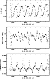 |
Fig. 7. Bottom panel: frequencies of single sine functions fitted to the SMEI data of ν Pup over time intervals of 75 d stepped by 10 d. Middle panel: as bottom panel, except for amplitudes. Top panel: O–C curve for a mean frequency of 0.655802 c/d. In all three panels, outliers have been clipped. |
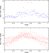 |
Fig. 8. Bottom panel: amplitudes from Fig. 7 phased with a frequency of 0.004186 c/d. Top panel: fitted amplitudes of the bottom panel phased with a frequency of 0.00130 c/d. |
Table 5 discloses that all SMEI frequencies in the group around 1.31 c/d can be derived with high fidelity from those in the group near 0.656 c/d. The frequencies c2 and c4 between the three harmonics c1, c3, and c5 are equal to the sum frequencies f1 + f2 and f2 + f3, respectively, to within the errors; they do not have counterparts in the 0.656-c/d group. Finally, the somewhat more distant c6 can be expressed as 2 × f2 + 4 × (f3 − f2). Given the numerous relations between all frequencies, this latter choice is necessarily not unique.
The described frequency scheme also suggests that – at the given photometric detection level – the groups of f1–f3 and c1–c5 are complete because the scheme and the frequencies in one group cannot be used to predict frequencies in the respective other group that are not observed. However, the presence of c6 suggests that a more complex extension to, or replacement of, the core scheme exists. In any event, additional variabilities will probably hide below the detection threshold of the BRITE and SMEI data. The variable shape of individual cycles of the light curve (Figs. 1 and 2) is presumably caused by the multiperiodicity. The persistence of the harmonic frequencies implies persistent asymmetries in agreement with Fig. 1.
A structure with two symmetric side lobes can arise in the power spectrum if a frequency and/or amplitude is modulated with the frequency difference between the central peak and the other two. If f1–f3 are exactly equidistant, as marginally permitted but not required by the time-series analysis, it needs to be determined whether the variability is due to a single but periodically modulated frequency or due to three separate frequencies. If only frequencies are considered, the problem is degenerate. An apparent advantage of the single-modulated-frequency hypothesis is that it easily explains c1–c5 if c3 is the harmonic of f2. Obviously, three separate frequencies cannot achieve this. Frequency c6 remains unexplained in both cases.
As a first step toward resolving this ambiguity, single-frequency sine fits to the SMEI data were performed in 75-d windows stepped by 10 d. The window of 75 d was chosen because it is about the shortest time interval over which meaningful fits of the 0.656 c/d variability can be obtained. It falls far short of resolving the 0.0021 c/d spacing. Figure 7 presents the results. The bottom panel suggests that the frequency is modulated with a quasiperiod near 480 d (0.0021 c/d). From the middle panel, one would infer that the amplitude varies about twice as fast as the frequency does. This double frequency is confirmed by a time-series analysis (Fig. 8). The amplitude of this amplitude modulation also varies cyclicly with 0.00013 c/d (Fig. 8). For a variable frequency, an O–C curve can be constructed which illustrates the difference between the observed phase (O; for instance measured as the times of maximal brightness) and that calculated (C) for the mean frequency. The O–C curve for f2 = 0.655802 c/d is depicted in the top panel, which seems to imply that there is a periodic ±0.2-d phase wobble.
Because frequencies f1–f3 alone are not sufficient to discriminate between one modulated and three separate frequencies, the usage for the above analysis of a single modulated frequency could be seen as introducing a bias. However, this choice is without prejudice to this issue, and the structures in Fig. 7 are of decisive diagnostic value in the analysis below (Sect. 3.3.2).
3.3.2. Simulations
Figure 7 makes it clear that a single modulated frequency would require a complex physical model to explain the large and conspicuous variations in amplitude and frequency. Moreover, the frequencies of these two quantities differ by a factor of approximately two (Figs. 7 and 8). Conjectures about such a model are deferred until simulations have investigated whether the structures in Fig. 7 are compatible with the alternative hypothesis of three separate3 frequencies. Because the observed frequencies are not unresolved blends (Sect. 3.2) and the sets of f1–f3 and c1–c5 appear complete (Sect. 3.3.1), simulated data should achieve acceptable approximations of the reality.
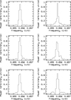 |
Fig. 10. Top left panel: power spectrum of SMEI observations between frequencies f1 and f3 (Table 5). Top right panel: as top left, except for combined SMEI and BRITE data. Other four panels: power spectra of a single sine function with frequency f2 evaluated at SMEI observing times. This variation is modulated with different amplitudes (A) and frequencies (F). 0.0003125 c/d is about the inverse of the time span of the SMEI observations. Middle left panel: A = 10 km s−1, F = 0.0003125 c/d; there is almost no difference w.r.t. the SMEI observations. Middle right panel: A = 30 km s−1, F = 0.0003125 c/d; the strength of the side lobes increases with the amplitude. Bottom left panel: A = 20 km s−1, F = 0.0003125 c/d; bottom right panel: A = 20 km s−1, F = 0.000625 c/d. The separation of main peak and side lobes increases with modulation frequency. |
A model with three constant frequencies (f1–f3), in other words, omitting the harmonics, was built from sine functions evaluated at the actual SMEI observing times. Amplitudes and phases were derived from single-frequency sine fits to the observations. The data were analyzed in exactly the same way as the real SMEI observations (Sect. 3.3.1). They are plotted in Fig. 9, which is not a fit but a proof of concept and as such demonstrates beyond any doubt that three separate frequencies can reproduce Fig. 7 in much detail.
In conclusion, the simulated data strongly favor the three-separate-frequencies option. An important and very firm outcome of the simulations is that the frequency doubling in the amplitude curve disappears when f1–f3 are truly equidistant. This is also analytically clear because, then, only one beat frequency exists. Therefore, f1–f3 are not exactly equidistant, which eliminates the need for the single-modulated-frequency conjecture altogether.
3.4. Mass loss
While BRITE can be effective at detecting photometric signatures of outbursts (Baade et al. 2018a,b), the extensive clipping applied to the SMEI observations of ν Pup may well have led to the removal also of genuinely stellar events. For the BRITE data of ν Pup, the detection threshold is lower but not by much because, for the stitching together of the numerous short data strings, it was assumed that between consecutive datasets there were no jumps intrinsic to the star.
By coincidence, the BHr2018 observations in the two bottom panels of Fig. 1 not only have the lowest instrumental scatter but were also obtained when the total photometric amplitude of ν Pup was lowest. These data should have the highest sensitivity to outbursts. Three peaks, consisting of four data points each, stand out above the ambient light curve by 5 mmag. They are the only candidate brightenings possibly related to mass loss that could be found. As the BHr2017 observations in Fig. 2 confirm, a 5-mmag offset of four consecutive data points each is significant, and the brightenings occurred well within an uninterrupted series of observations. However, non-Gaussian errors do occur, and it would require simultaneous observations with two instruments to ascertain (or not) the reality of such events. Owing to the beating with much larger amplitude, even two BRITE satellites would probably find it difficult to identify events of similar magnitude but ten times longer duration as seen in the B5e star KIC 11971405 (Kurtz et al. 2015; Rivinius et al. 2016).
3.5. Binarity
A late-type, that is, low-mass, Be star such as ν Pup might offer an opportunity to derive useful constraints on the presence of a companion star. Pulsation-induced variations and circumstellar components of line profiles are a lesser problem than in early-type Be stars. However, strong rotational line broadening and the paucity of suitable spectral lines pose other challenges, as also seen in ν Pup. Photometric Doppler variations can, therefore, be a useful alternative to conventional spectroscopy, especially since accurate measurements of multi-frequency variations necessarily require excellent phase coverage.
An elaborate description of the power of photometric Doppler shifts for the analysis of binaries with pulsating component(s) is available from Shibahashi et al. (2015) and references therein. Here, only the most basic application is used. Figure 10 derives, in the low-frequency regime, an upper limit of ∼20 km s−1 on the amplitude of sinusoidal radial-velocity variations and illustrates that frequencies down to about 0.0006 c/d (periods up to ∼4.5 years) can be excluded. The location of f1 and f3 at a separation from f2 of about ±0.0021 c/d (see left panel of Fig. 11) leads to a blind spot of the method around that frequency. The right panel of Fig. 11 presents the simulated power spectrum around f2 for a 1-M⊙ star orbiting ν Pup at a distance of 1 au (period nearly half a year; frequency ∼0.0057 c/d). Because of the extreme contrast in the observations between the peak at 0.655802-c/d and all other features (see left panel of Fig. 11), it would be possible to identify the two weak spikes at 0.6558 ± 0.0057 c/d.
In the IUE spectra, evidence of a hot companion was not found. From cross-correlation of the observations with the hottest model template spectrum (45 kK) only an upper limit of ∼2% of the flux of the Be primary could be derived for the secondary. The signal-to-noise ratio of 2.49 is below the significance threshold of 3.0 established by Wang et al. (2018). The low temperature of the primary also enabled the usage of templates corresponding to temperatures of 35 and 27.5 kK. The resulting cross-correlation functions are broader than that with the 45 kK template (Fig. 12) because of stronger similarities with the B-type primary. In the classification scheme of Wang et al. (2018), ν Pup would be assigned code “P” (cross-correlation signal from primary star).
Finally, the HIPPARCOS and the Gaia DR2 parallaxes agree very well. This may also indicate that, on timescales of few years, there is no strong orbital reflex motion caused by an unseen companion.
4. Discussion
Except for its intermittent shell-star nature, ν Pup seems to be a normal B7-B8 IIIe star. A magnetic field was not detected. High-quality spectra exhibited no abundance anomalies or other pecularities. The upper limit on periodic sinusoidal RV variations is 10 km s−1 (Sect. 3.1). For amplitudes in that range, periods up to a few years appear ruled out (Sect. 3.5). Weak emission and shell absorption components in Hα (Rivinius et al. 1999) were observed between 1995 and 1999; they may have marked the end of the disk dissipation period after stronger emission a decade before.
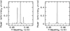 |
Fig. 11. Left panel: same as top left panel of Fig. 10 except for compressed abscissa. Right panel: same as lower four panels of Fig. 10 except for compressed abscissa and A = 12 km s−1 and F = 0.0057 c/d, corresponding to a 1-M⊙-star orbiting ν Pup at 1 au. In the left panel, f1–f3 (Table 5) are visible whereas the synthetic data in the right panel only include f2 and its side lobes due to the assumed orbital motion. |
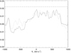 |
Fig. 12. Cross-correlation functions between the two IUE observations of ν Pup and the 45 kK model template as described in Sect. 3.5. Because of different degrees of similarity to the spectrum of the Be primary, the cross-correlation functions for the 45 kK template are narrower than those with the 35 kK and 27.5 kK templates. The horizontal line indicates a signal-to-noise ratio level of 3.0 above which a companion with temperature ∼45 kK would be considered significant. |
The detection with photographic plates of shell absorption in Hγ (Wright 1909) implies that either 80–90 years earlier the circumstellar disk was much more developed or in the 1990’s the peak of the emission phase was, in fact, missed. The complete absence of Hα line emission in the years 2000, 2005, and 2016 (see Table 3) may be a weak indication that a good part of the SMEI (2003–2011) and BRITE (2015, 2016/17, and 2017/18) observations perhaps took place while ν Pup did not maintain a disk of much significance. For the HIPPARCOS data, no parallel spectroscopic record exists; however, in the 1989–1993 time interval the disk may have been dissipating (Sect. 3.1). Accordingly, the persistent, regular variability seen with SMEI or BRITE should be of primarily stellar – instead of circumstellar – nature.
The tight and homogeneous frequency pattern evidences that the entire variability is intrinsic to one single star. There is no contamination by a companion or field star. Frequencies f1–f3 and c1–c5 seem to be complete sets in that no frequencies following the construction scheme of Table 5 are missing (Sect. 3.3.1). The frequencies found are not compromised by unresolved blends (Sect. 3.2).
Simulations (Sect. 3.3.2) have demonstrated that the 0.656-c/d variability consists of three separate frequencies (f1–f3). There is also no physical motivation to consider frequency modulation with 0.0021 c/d: Binary models are rejected in Sects. 3.5 and 4.4, and 0.02 d cannot possibly be the light travel time in a binary because the implied mass would be superstellar. Oblique rotators are ruled out because a splitting by 0.0021 c/d would imply a rotation rate that is two orders of magnitude below the observed line width. A rapidly rotating magnetic oblique pulsator would require a very strong magnetic field that is not observed. A complex differential-rotation scheme can be construed but the fine tuning introduces more challenges than it can eliminate. Intrinsic frequency variations are known from other stars and mostly thought to result from pulsation-mode interactions. The most notable example is the Blazhko effect, for example, in RR Lyr (Prudil & Skarka 2017) and δ Cephei (Smolec 2016) stars. However, it seems to involve one or more radial modes, which are not known from Be stars (Sect. 4.1).
In conclusion, not only does the three-separate-frequencies model reproduce the observations well but there is also no physical need to add extrinsic or intrinsic long-term variability. Therefore, the interpretation is adopted that the 0.656-c/d variability of ν Pup consists of three separate variations. Without regard to this splitting, possible identifications of this variability are briefly discussed in the next subsection.
4.1. Possible causes of the 0.656-c/d variability
Radial pulsation. There is apparently no case of reported radial pulsation in Be as well as SPB stars. This is in agreement with model calculations which consistently find radial modes strongly damped at the temperature of ν Pup (e.g., Pamyatnykh 1999). For ν Pup, a drastic mismatch exists w.r.t. the mean pulsation constant Q = 0.033 d for the radial modes of β Cep (and similarly many other) stars (Stankov & Handler 2005). In conclusion, the 0.656-c/d frequency of ν Pup is not due to radial pulsation.
Circumstellar Štefl frequency. Some Be stars exhibit a so-called Štefl frequency (Štefl et al. 1998; Baade et al. 2016). In spectroscopy, Štefl frequencies are most prominent in lines formed in the photosphere-to-disk transition region. Their amplitude seems to trace the star-to-disk mass transfer rate as is inferred from the nondetection of Štefl frequencies at times when the Hα line emission is weak or fading. However, the yearslong absence in ν Pup of Hα line emission and especially the concomitant disappearance and subsequent absence for perhaps >15 years also of shell absorption in this equator-on star argues against the interpretation as a Štefl frequency of the 0.656-c/d variability. In conclusion, the hypothesis of a circumstellar Štefl frequency for the 0.656-c/d variability lacks merit.
Rotational modulation. The initial confusion of nonradial pulsation with magnetic rotational modulation (Balona 2013, and references therein) has long been resolved (Rivinius 2013). Nevertheless, the possibility of rotational modulation cannot be fundamentally excluded. Often in Be stars, plausible rotation frequencies are embedded in frequency groups which makes the identification of the former somewhat arbitrary (e.g., Diago et al. 2009). Beyond such coincidences, rotational modulation of specific properties (e.g., line strengths of specific elements) has not been reported. In ν Pup, the observed frequency of 0.656 c/d is straddled by the model rotation rate of 0.5 c/d (Table 2) and the rotation rate 0.77 c/d derived from the observed rotational velocity of 246 km s−1 (Royer et al. 2002) and the also calculated equatorial radius of 6.85 R⊙ (which is supported by the observed parallax). In conclusion, rotational modulation is well possible but not positively demonstrated. The lack of spectroscopic fiducial marks (Sect. 3.1) carried around the star is an obstacle.
Ellipsoidal variability in a binary. In such systems, the photometric frequency is usually twice the orbital frequency so that in ν Pup the orbital frequency would be 0.33 c/d. If the putative companion is a white dwarf with mass 0.5 M⊙ in a circular orbit, the orbital velocity of the Be primary would be about 30 km s−1. Although noisy, the radial-velocity curve in Fig. 4 and the photometric Doppler simulations (Sect. 3.5) do not harbor a 2 × 30 km s−1 variability. The expected semi-amplitude could be lower if spin and orbit are misaligned. However, the compilation by Albrecht et al. (2011) suggests that major misalignments do not occur in binaries of similar period. The kink near the maximum of the light curve (Fig. 2) could also be a secondary minimum which could be shallower than the primary minimum if the photospheric regions facing toward and away from the companion have different surface brightnesses. In that case, the orbital frequency would be 2 × 0.33 c/d, much aggravating the radial-velocity problem, and the separation of the two stars would shrink to little more than the sum of the equatorial radii in Table 2. The emission could, then, only arise in a circumbinary disk formed by Roche-lobe overflow. In conclusion, ν Pup is not likely to be an ellipsoidal variable in agreement with the general arguments presented in Sects. 3.5 and 4.4 against ν Pup being a double star.
4.2. Nonradial pulsation
None of the options considered for the 0.656-c/d variability (Sect. 4.1) has a built-in mechanism to explain the splitting into f1–f3, thereby further aggravating the strong tension with the observations. Frequency groups are widespread in Be stars (cf. Introduction) and are commonly attributed to multi-mode nonradial pulsation.
Frequency groups can be difficult to delineate but typically three of them are found. Kurtz et al. (2015) suggested that the grouping could arise from combination frequencies. Pápics et al. (2017) found this tendency confirmed among the more than 1000 frequencies diagnosed in the same data. The preliminary picture presented by Baade et al. (2018b) of the B1 Ve star 25 Ori is similar. There is no explanation yet of the formation, prominence, and role of combination frequencies in Be stars as pictured below. The most elementary empirical description that can be given of frequency groups is that one group (g1) consists of the NRP frequencies proper and groups g0 and g2 are built from differences and sums and/or harmonics, respectively, of frequencies in g1. However, in the presence of noise and finite frequency resolution, a firm and satisfactorily complete classification of a rich frequency spectrum is not straightforward.
The small number of frequencies detected in ν Pup facilitates this task a lot, and Table 5 provides the most complete characterization to date of frequency groups in Be stars. Group g1 consists of f1–f3 whereas all six members c1–c6 of group g2 are sum or harmonic frequencies of f1 through f3. The NRP hypothesis makes it thus possible (but not necessary), by analogy to other Be stars, to construct c2 and c4 as sum frequencies f1 + f2 and f2 + f3, respectively. This possibility would remove the last deficiency of the three-separate-frequencies model with respect to the single-modulated-frequency hypothesis. It provides additional motivation to prefer a triple NRP-mode interpretation for f1–f3.
Group g0 is empty; this lack of difference frequencies (they would occur around 0.0021 c/d) is perhaps not surprising because, in more active early-type Be stars, they are often associated with repetitive brightening events that probably signal mass- and angular-momentum-loss episodes. ν Pup is a very inactive late-type Be star with mass-loss events possibly occurring as rarely as every couple of decades.
The NRP diagnosis is consistent with standard properties of NRPs in B-type stars. ν Pup is located near the cool high-luminosity “corner” of the OPLIB SPB instability strip calculated by Walczak et al. (2015). The by far most detailed study to date of the photometric variability of a mid-type Be star is that of KIC 11971405 by Pápics et al. (2017). These authors identify what they call the “independent pulsation modes” (group g1 in the above terminology) of KIC 11971405 in the range 1.3–2.3 c/d. Considering the difference in spectral type, B7-8 IIIe (ν Pup) vs. B5 IV-Ve (KIC 11971405), 0.656 c/d is a plausible frequency for NRP modes in ν Pup.
The variability of ν Pup is somewhat similar to that of HD 175869: This latter star exhibits a single frequency at 0.639 c/d and a first harmonic with amplitude of more than 50% of the base variability. However, at 0.111 and 0.197 mmag, respectively, (Gutiérrez-Soto et al. 2009) they are approximately two orders of magnitude lower than the amplitudes in ν Pup. Higher harmonics were also reported for HD 175869 albeit at very low levels. Because the observations only extend over 27.3 days, very closely spaced triple-frequency structures such as in ν Pup could not be detected so that it is not known whether the also reported amplitude variability is real or caused by a nearby but unresolved frequency. It also remains unclear what the impact of undetected frequency multiplicity would be on the seismic modeling performed by Neiner et al. (2012).
The photometric amplitudes of nonradially pulsating stars depend on the mode type and inclination angle. Rivinius et al. (2003) found that the dominating line-profile variability of most early-type Be stars is best modeled with retrograde quadrupole NRP modes (ℓ = |m| = 2). Because of the equator-on perspective implied by the temporary presence of shell lines, such modes can attain large photometric amplitudes in ν Pup (Daszyńska-Daszkiewicz et al. 2007). By contrast, the spectroscopic sensitivity to such modes is low at inclinations close to 90° (Rivinius et al. 2003), and any multi-mode NRP would further dilute the spectroscopic signatures. Therefore, the lack of detection of the latter (Sect. 3.1) is not a model-discriminating diagnostic.
It is interesting to consider how the actually observed frequencies in a group are selected from all the other possibilities. This is a variant of the more general question of why it is often only a few modes from the very dense NRP frequency spectra of B stars that dominate the observed power spectrum, and why is it those that do? As Table 5 proves, the frequencies in ν Pup are extremely tightly coupled. Either the strength of this coupling or the strength of the pulsations, or both, may be responsible for the strong and variable asymmetry of the individual cycles of the light curve (Figs. 1 and 2). It may be frequency differences like 0.0021 c/d in ν Pup that act as mode couplers and selectors because in some Be stars half a dozen pairs of apparent NRP modes share the same difference frequency (Baade et al. 2018b). Another selection or combination rule seems to be that only modes with the same angular eigenfunction combine in an appreciable way (Baade 1998) in mass-loss events.
The strength of coupling of g-modes scales with the square of the rotation rate and becomes relevant for modes more closely spaced than the rotational splitting. The spacing of ∼0.0021 c/d is way below this threshold. For the principles and examples of g-mode coupling, see Soufi et al. (1998) and Daszyńska-Daszkiewicz et al. (2002), respectively.
Through combination frequencies shared by many pairs of NRP modes, single NRP frequencies can be assembled to intricate nested clockworks that open and close the mass- and probably also angular-momentum-loss valves of Be stars. A rich example is 25 Ori (Baade et al. 2018b). If selected difference frequencies act as mode couplers and selectors also in ν Pup, any mass-loss events from first-level difference frequencies (∼0.0021 c/d) and the NRP modes involved in them may be below the detection limits of SMEI and BRITE. (A speculative complementary description of the mass loss from ν Pup is outlined in Sect. 4.3.) Undetected low-amplitude variabilities may also explain the very low relative widths of the two frequency groups in ν Pup. At Δf/f ≪ 1%, they are narrower by much more than an order of magnitude than typical frequency groups in other Be stars. The narrowness of the groups could be just the result of the close subgrouping of these high-amplitude frequencies.
This latter conclusion is supported by the case of the pulsating Be star 25 Ori where three similar triple-frequency structures appear in the power spectrum (Baade et al. 2018b, Baade et al., in prep.). All three have the spacing of 0.0129 c/d in common and, together with additional, weaker features, form frequency subgroups, which are correspondingly narrow but still more than six times as wide as the f1–f3 complex in ν Pup. Two of them fall into g1, one belongs to g2. However, there are no detectable harmonics.
Although 0.0021 c/d is not detected as a difference frequency, the clustering near 0.0021 c/d of frequency differences in ν Pup invites comparisons to accumulations of frequency differences seen in other Be stars. In 25 Ori (Baade et al. 2018b), at least two clusters of frequency differences exist, with complex connections and interactions between them. Simpler patterns have been found in η Cen (Baade et al. 2016) and 28 Cyg (Baade et al. 2018a). Therefore, this and other mode-selection rules in Be stars may be the DNA of the stellar part of the Be phenomenon, and 25 Ori and ν Pup span much of the range of variability patterns in Be stars. 25 Ori undergoes cyclicly repeating outbursts, probably governed by a hierarchical set of NRP-controlled clocks (Baade et al. 2018b). This persistent activity may lead to the appearance of additional frequencies, which has been proposed to happen during outbursts (Huat et al. 2009; Baade et al. 2018a). ν Pup harbors a similar clockwork, and the main difference may be that the observations presented of ν Pup depict such a clockwork during quiescence and not obliterated by the mass-ejection process.
4.3. Mass loss
The temporary presence in ν Pup of line emission and shell absorption in Hα, however exiguous they were, requires some (variable) mass-loss mechanism. The latter cannot be founded on rotation or radiation alone or their combination. A good fraction of the mass loss from Be stars may take place in discrete events (cf. Introduction). However, both photometry and spectroscopy suggest that, in ν Pup, major events happened at most once per decade. According to model calculations by Haubois et al. (2012), mass-loss events in equator-on stars like ν Pup are effective in letting the circumstellar disk remove part of the stellar flux. No major dimming event was seen in many years of photometry which, however, were limited in their sensitivity to such variations. There may be brightenings by a few mmag and for a fraction of a day. If they do present mass-loss events, the amounts of matter ejected per event must be very small. But there could be of order 102 such events per year.
A rate of one larger outburst or less per decade is within the findings of Bernhard et al. (2018) for late-type Be stars who, in grund-based data, had lower sensitivity to outbursts than this study of ν Pup has. Without replenishment, the disk is disrupted by viscous re-accretion as well as viscous expansion into the interstellar medium (Vieira et al. 2017). Given the low UV flux of B8 stars, additional radiative demolishment (Kee et al. 2018, and references therein) is comparatively unimportant. Accordingly, unperturbed disk dissipation times can be measured, providing important constraints on temporal and spatial variations of the viscosity. Alternatively, one might have to infer a more continuous star-to-disk mass-transfer process that is too weak to be detected by the most common observing techniques. For experimental verification in the optical, linear continuum (Guinan & Hayes 1984; Carciofi et al. 2007) and line polarimetry is more sensitive to near-stellar matter than plain photometry or spectroscopy are.
If clusters of frequency differences are involved in the mass loss from ν Pup, the only possible choice offered by the observations is 0.0021 c/d. During the time of the observations the corresponding difference frequencies were not detectable because the conditions for the driving of mass loss were not met. If the condition for outbursts of ν Pup is that all of f1–f3 are in phase, and if f1–f3 are unequally spaced, the implied timescale is 40 years. This is not too different from the separation in time of the two shell phases. The latter interval amounts to 80–90 years (Sect. 4), and another event in between would have gone unnoticed for lack of observations. ν Pup could, then be another illustration of hierachically nested clocks that drive mass loss from Be stars (Baade et al. 2018b). At the lowest clock level ℓ1, there are the NRP modes in g1. At the third level ℓ3, there is the difference between the two difference frequencies f2 – f1 and f3 – f1, which both form the second level ℓ2. The orders of magnitude of the three time scales are a day, a year, and some decades, respectively, for ℓ1, ℓ2, and ℓ3. Apparently, clock level ℓ2 has no effect on mass loss, certainly not at a level of magnitude detectable by spectroscopy. By analogy to 25 Ori, the two difference frequencies would attain high amplitudes only for a few weeks or even less (they are not simple beat frequencies). When the two are roughly in phase, the mass-loss valve opens and the two difference frequencies drive the mass loss.
4.4. Binarity
The origin of the rapid rotation of Be stars is not known. In observations of open star clusters, it has been found that Be stars already have high angular momentum when they reach the zero-age main sequence (Martayan et al. 2007, and references therein). However, it has also been variously suggested (Pols et al. 1991; Harmanec et al. 2002; Boubert & Evans 2018, and references therein) that binarity plays a formative role in the Be phenomenon. In fact, Be stars with subluminous companions (Wang et al. 2018) and Be X-ray binaries with compact companions (Reig 2011) prove that there are Be stars that must have gone through a phase of strong interactions with these companion stars. Accordingly, many Be stars probably acquired (much of) their high angular momentum through mass transfer from a another star. On the other hand, just one case of an effectively single Be star without high space velocity (which could arise if a supernova explosion had disrupted a former binary) would demonstrate that there must be both double- and single-star evolutionary paths toward the Be phenomenon. If Be stars do form in more than one way, it will be very stimulating to learn whether the pulsations of Be stars can be tracers of these formation processes.
In order to consider a Be star effectively single, its separation should probably be at least one astronomical unit. The presumably best-determined mass and orbit of a supposed sdO companion to a Be star are that of the B2 Ve star ϕ Per with 1.2 M⊙ and orbital period of 127 d (Mourard et al. 2015). It seems feasible to rule out such a star in ν Pup (Sect. 3.5), using limits on photometric Doppler shifts. With precise modeling and stacking of suitable features in the power spectrum, even lower detection limits appear possible. However, companions with masses as low as 0.07 M⊙ have been reported, based on up to 88 IUE spectra (Peters et al. 2016, HR 2142, B1.5 IV-Vnne). Such masses do not seem to be within reach of current ν Pup photometry. Application of the same technique to the IUE spectra of the much cooler star ν Pup should help. However, with two spectra alone, comparable sensitivity cannot be achieved. Nevertheless, ν Pup appears as one of the best targets for efforts aiming at the first identification of an effectively single Be star.
At 30–35 km s−1, the radial velocity is relatively high; the plane-of-sky component of ∼3 km s−1 derived from the Gaia parallax and proper motion (Gaia Collaboration 2018) only adds little to the space velocity. This velocity could be the result of the break-up of a former binary if the more massive star underwent a supernova explosion. Since ν Pup traverses the current distance of ∼110 pc from the solar system in about 3.5 × 10⁶ years, no spectacular event would be implied. However, for a single object, nothing can be said about any earlier mass and angular-momentum transfer to the Be star from an assumed exploded star.
5. Conclusions
Significant photometric coverage from space of the variability of ν Pup is available over a time spanning three decades (1989 through 2018). This has permitted an unprecedented study of the long-term behavior of the variability of a Be star.
ν Pup is a B7-B8 IIIe star without detected spectroscopic anomalies other than the rare line-emission and shell phases. It exhibits a ∼10-mmag variability near 0.6556 c/d split into three frequencies f1–f3 spaced by ∼0.0021 c/d. The frequency spacing is nearly but not exactly equidistant; neither appear the periods equidistant. Five much weaker variabilities form a second nearly equidistant frequency group near 1.31 c/d; three of them are harmonics of f1–f3. Similarly narrow groups of high-amplitude NRP modes are not known from other Be stars unless similar frequency groups in HD 175869 were not resolved with the one-month observations (Gutiérrez-Soto et al. 2009). However, the narrowness may be the result of the insensitivity of the observations to sub-mmag variations. The frequency spacing is very much smaller than any expected rotational splitting of NRP modes.
The similarity of the spacing between all frequencies in both groups suggests that they are somehow coupled. This coupling along with the large amplitudes may be responsible for the strong and varying asymmetry of the light curve.
In early-type Be stars, difference frequencies seem to be involved in the triggering of mass-loss events. The existence of very effective selection rules of NRP modes, which are also implied by other observations, may be part of the DNA of the stellar component of the Be phenomenon. Because the mass-loss process in ν Pup is very weak but frequency combinations are still very prominent, NRP-enabled mass loss from Be stars should only be the consequence of coupled NRP modes, not also their cause. A causal element may lie in the radial transport of excess angular momentum. Because Be stars are not destroyed by the angular momentum rising to the surface, the unknown mode-selection process may favor difference frequencies effective in preventing an angular-momentum catastrophe.
Before the availability of space photometry, Be stars were notorious for their seemingly unpredictable, erratic behavior. Satellite observations have revealed complex variability patterns, which can be governed by multiply nested clocks and can, therefore, be repetitive. However, the duration of observations required to recognize such repetitive patterns is long, especially if multiple and/or closely spaced frequencies rule the light curve. The 0.0021-c/d frequency spacing in ν Pup has extended the range of these timescales to ∼1000 d. The synchronization over two very similar ∼0.0021-c/d beat cycles in ν Pup of f1–f3 takes decades, possibly in agreement with the spacing of shell episodes.
Late-type Be stars are also a source of valuable observational data for the analysis of the disk dissipation process: Compared to hotter Be stars, radiative effects on the disk are much lower, the dissipation is much less likely to be disturbed or reversed by new outbursts, and the sensitivity to a continuous star-to-disk mass-transfer process, if any, could be much higher. This may enable a more precise determination of the viscosity parameter, its radial and vertical distribution in the disk, and its temporary evolution (cf. the work on the early-type Be star 28 CMa by Ghoreyshi et al. 2018).
Motivated by the expectation that Be stars result from the evolution of binary stars, searches have been carried out, and many actual and candidate binary systems have been identified. It would be most valuable to complement such efforts with deep analyses of a few Be stars with the goal of finding out whether effectively single Be stars also exist. The edge-on perspective, relatively low mass, very large photometric amplitude, and simple frequency spectrum render ν Pup a promising test target. By the example of ν Pup it could be shown, for the first time in Be stars, that photometric Doppler shifts can place useful constraints on the properties of companion stars. Other Be stars worth investigating in this way include KIC 11971405 and Achernar (Goss et al. 2011). Achernar does have a known companion. However, at an estimated separation of 6.7 au (Kervella et al. 2008), Achernar should still pass as effectively single if no closer companion exists. If effectively single Be stars can be identified, it will be most illuminating to learn whether pulsations can distinguish the formation histories of different populations of Be stars.
Acknowledgments
The authors are immensely indebted to Professor Bernard V. Jackson for the provision of the newly processed SMEI observations. They thank the BRITE operations staff for their untiring efforts to deliver data of the quality that enabled this investigation. Dr. Coralie Neiner is gratefully acknowledged for the in-advance communication (through GAW) of the results of the magnetic-field measurement. The Polish contribution to the BRITE project is supported by Polish Ministry of Science and Higher Education, and the Polish National Science Center (NCN, grant 2011/01/M/ST9/05914). This research has made use of the SIMBAD database, operated at CDS, Strasbourg, France. This research has made use of NASA’s Astrophysics Data System. This work is partly based on observations obtained at the Canada-France-Hawaii Telescope (CFHT) which is operated by the National Research Council of Canada, the Institut National des Sciences de I’Univers of the Centre National de la Recherche Scientifique of France, and the University of Hawaii. The CFHT data were obtained from the Canadian Astronomy Data Centre operated by the National Research Council of Canada with the support of the Canadian Space Agency. Some of the data presented in this paper were obtained from the Mikulski Archive for Space Telescopes (MAST). STScI is operated by the Association of Universities for Research in Astronomy, Inc., under NASA contract NAS5-26555. Support for MAST for non-HST data is provided by the NASA Office of Space Science via grant NNX09AF08G and by other grants and contracts. ACC acknowledges support from CNPq (grant307594/2015-7). GH thanks the Polish NCN for support (grant 2015/18/A/ST9/00578). AFJM is grateful for financial aid from NSERC (Canada) and FRQNT (Quebec). APi acknowledges support from the Polish NCN grant no. 2016/21/B/ST9/01126. DP acknowledges financial support from Conselho Nacional de Desenvolvimento Científico e Tecnológico (CNPq-MCTIC Brazil; grant 300235/2017-8). SMR and GAW acknowledge Discovery Grant support from the Natural Sciences and Engineering Research Council (NSERC) of Canada. KZ acknowledges support by the Austrian Fonds zur Förderung der wissenschaftlichen Forschung (FWF, project V431-NBL) and by the Austrian Forschungsförderungsgesellschaft (FFG).
References
- Albrecht, S., Winn, J. N., Carter, J. A., Snellen, I. A. G., & de Mooij, E. J. W. 2011, ApJ, 726, 68 [NASA ADS] [CrossRef] [Google Scholar]
- Baade, D. 1989a, A&AS, 79, 423 [NASA ADS] [Google Scholar]
- Baade, D. 1989b, A&A, 222, 200 [NASA ADS] [Google Scholar]
- Baade, D. 1998, in New Eyes to See Inside the Sun and Stars, eds. F. L. Deubner, J. Christensen-Dalsgaard, & D. Kurtz, IAU Symp., 185, 347 [NASA ADS] [Google Scholar]
- Baade, D., Rivinius, T., Pigulski, A., et al. 2016, A&A, 588, A56 [NASA ADS] [CrossRef] [EDP Sciences] [Google Scholar]
- Baade, D., Rivinius, T., & Pigulski, A. 2017, in Second BRITE-Constellation Science Conf.: Small Satellites – Big Science, eds. K. Zwintz, & E. Poretti, Proc. Polish Astron. Soc., 5, 196 [Google Scholar]
- Baade, D., Pigulski, A., Rivinius, T., et al. 2018a, A&A, 610, A70 [NASA ADS] [CrossRef] [EDP Sciences] [Google Scholar]
- Baade, D., Rivinius, T., & Pigulski, A. 2018b, 3rd BRITE Science Conference, 8, 69 [NASA ADS] [Google Scholar]
- Balona, L. A. 2013, in Stellar Pulsations: Impact of New Instrumentation and New Insights, eds. J. C. Suárez, R. Garrido, L. A. Balona, & J. Christensen-Dalsgaard, Astrophys. Space Sci. Proc., 31, 247 [NASA ADS] [CrossRef] [Google Scholar]
- Balona, L. A., Pigulski, A., Cat, P. D., et al. 2011, MNRAS, 413, 2403 [NASA ADS] [CrossRef] [Google Scholar]
- Banse, K. 2003, Inf. Handling Astron. Historical Vistas, 285, 89 [NASA ADS] [CrossRef] [Google Scholar]
- Barnsley, R. M., & Steele, I. A. 2013, A&A, 556, A81 [NASA ADS] [CrossRef] [EDP Sciences] [Google Scholar]
- Berghoefer, T. W., Schmitt, J. H. M. M., & Cassinelli, J. P. 1996, A&AS, 118, 481 [NASA ADS] [CrossRef] [EDP Sciences] [Google Scholar]
- Bernhard, K., Otero, S., Hümmerich, S., et al. 2018, MNRAS, 479, 2909 [NASA ADS] [CrossRef] [Google Scholar]
- Bodensteiner, J., Baade, D., Greiner, J., & Langer, N. 2018, A&A, 618, A110 [NASA ADS] [CrossRef] [EDP Sciences] [Google Scholar]
- Boggess, A., Carr, F. A., Evans, D. C., et al. 1978, Nature, 275, 372 [NASA ADS] [CrossRef] [Google Scholar]
- Boubert, D., & Evans, N. W. 2018, MNRAS, 477, 5261 [NASA ADS] [CrossRef] [Google Scholar]
- Cameron, C., Saio, H., Kuschnig, R., et al. 2008, ApJ, 685, 489 [NASA ADS] [CrossRef] [Google Scholar]
- Carciofi, A. C., Magalhães, A. M., Leister, N. V., Bjorkman, J. E., & Levenhagen, R. S. 2007, ApJ, 671, L49 [NASA ADS] [CrossRef] [Google Scholar]
- Cousins, A. W. J. 1987, S. Afr. Astron. Observ. Circ., 11, 93 [NASA ADS] [Google Scholar]
- Daszyńska-Daszkiewicz, J., Dziembowski, W. A., Pamyatnykh, A. A., & Goupil, M.-J. 2002, A&A, 392, 151 [NASA ADS] [CrossRef] [EDP Sciences] [Google Scholar]
- Daszyńska-Daszkiewicz, J., Dziembowski, W. A., & Pamyatnykh, A. A. 2007, Acta Astron., 57, 11 [NASA ADS] [Google Scholar]
- Diago, P. D., Gutiérrez-Soto, J., Auvergne, M., et al. 2009, A&A, 506, 125 [NASA ADS] [CrossRef] [EDP Sciences] [Google Scholar]
- Donati, J. F., Catala, C., Landstreet, J. D., & Petit, P. 2006, in Solar Polarization, eds. R. Casini, & B. W. Lites, ASP Conf. Ser., 358, 362 [Google Scholar]
- Ducati, J. R. 2002, VizieR Online Data Catalog: II/237 [NASA ADS] [Google Scholar]
- Eggleton, P. P., & Tokovinin, A. A. 2008, MNRAS, 389, 869 [NASA ADS] [CrossRef] [Google Scholar]
- ESA 1997, VizieR Online Data Catalog: I/239 [Google Scholar]
- Frémat, Y., Zorec, J., Hubert, A.-M., & Floquet, M. 2005, A&A, 440, 305 [NASA ADS] [CrossRef] [EDP Sciences] [Google Scholar]
- Gaia Collaboration 2018, VizieR Online Data Catalog: I/345 [Google Scholar]
- Ghoreyshi, M. R., Carciofi, A. C., Rímulo, L. R., et al. 2018, MNRAS, 479, 2214 [NASA ADS] [CrossRef] [Google Scholar]
- Goss, K. J. F., Karoff, C., Chaplin, W. J., Elsworth, Y., & Stevens, I. R. 2011, MNRAS, 411, 162 [NASA ADS] [CrossRef] [Google Scholar]
- Granada, A., Ekström, S., Georgy, C., et al. 2013, A&A, 553, A25 [NASA ADS] [CrossRef] [EDP Sciences] [Google Scholar]
- Guinan, E. F., & Hayes, D. P. 1984, ApJ, 287, L39 [NASA ADS] [CrossRef] [Google Scholar]
- Gutiérrez-Soto, J., Floquet, M., Samadi, R., et al. 2009, A&A, 506, 133 [NASA ADS] [CrossRef] [EDP Sciences] [Google Scholar]
- Harmanec, P., Bisikalo, D. V., Boyarchuk, A. A., & Kuznetsov, O. A. 2002, A&A, 396, 937 [NASA ADS] [CrossRef] [EDP Sciences] [Google Scholar]
- Haubois, X., Carciofi, A. C., Rivinius, T., Okazaki, A. T., & Bjorkman, J. E. 2012, ApJ, 756, 156 [NASA ADS] [CrossRef] [Google Scholar]
- Haubois, X., Mota, B. C., Carciofi, A. C., et al. 2014, ApJ, 785, 12 [Google Scholar]
- Hick, P., Buffington, A., & Jackson, B. V. 2007, in Solar Physics and Space Weather Instrumentation II, Proc. SPIE, 6689, 66890C [Google Scholar]
- Howarth, I. D., & Stevens, I. R. 2014, MNRAS, 445, 2878 [NASA ADS] [CrossRef] [Google Scholar]
- Huat, A.-L., Hubert, A.-M., Baudin, F., et al. 2009, A&A, 506, 95 [NASA ADS] [CrossRef] [EDP Sciences] [Google Scholar]
- Hubert, A. M., & Floquet, M. 1998, A&A, 335, 565 [NASA ADS] [Google Scholar]
- Jackson, B. V., Buffington, A., Hick, P. P., et al. 2004, Sol. Phys., 225, 177 [Google Scholar]
- Kaufer, A. 1998, in Star and Galaxies, ed. R. E. Schielicke, Rev. Mod. Astron., 11, 177 [NASA ADS] [Google Scholar]
- Kee, N. D., Owocki, S., & Kuiper, R. 2018, MNRAS, 474, 847 [NASA ADS] [CrossRef] [Google Scholar]
- Kervella, P., de Domiciano Souza, A., & Bendjoya, P. 2008, A&A, 484, L13 [NASA ADS] [CrossRef] [EDP Sciences] [Google Scholar]
- Koen, C., & Eyer, L. 2002, MNRAS, 331, 45 [NASA ADS] [CrossRef] [Google Scholar]
- Krtička, J. 2014, A&A, 564, A70 [NASA ADS] [CrossRef] [EDP Sciences] [Google Scholar]
- Krtička, J., Owocki, S. P., & Meynet, G. 2011, A&A, 527, A84 [NASA ADS] [CrossRef] [EDP Sciences] [Google Scholar]
- Kurtz, D. W., Shibahashi, H., Murphy, S. J., Bedding, T. R., & Bowman, D. M. 2015, MNRAS, 450, 3015 [NASA ADS] [CrossRef] [Google Scholar]
- Lanz, T., & Hubeny, I. 2003, ApJS, 146, 417 [NASA ADS] [CrossRef] [Google Scholar]
- Lesh, J. R. 1968, ApJS, 17, 371 [NASA ADS] [CrossRef] [EDP Sciences] [Google Scholar]
- Martayan, C., Frémat, Y., Hubert, A.-M., et al. 2007, A&A, 462, 683 [NASA ADS] [CrossRef] [EDP Sciences] [Google Scholar]
- Meilland, A., Millour, F., Kanaan, S., et al. 2012, A&A, 538, A110 [NASA ADS] [CrossRef] [EDP Sciences] [Google Scholar]
- Mourard, D., Monnier, J. D., Meilland, A., et al. 2015, A&A, 577, A51 [NASA ADS] [CrossRef] [EDP Sciences] [Google Scholar]
- Mowlavi, N., Barblan, F., Saesen, S., & Eyer, L. 2013, A&A, 554, A108 [NASA ADS] [CrossRef] [EDP Sciences] [Google Scholar]
- Neiner, C., Mathis, S., Saio, H., et al. 2012, A&A, 539, A90 [NASA ADS] [CrossRef] [EDP Sciences] [Google Scholar]
- Neiner, C., Mathis, S., Saio, H., & Lee, U. 2013, in Progress in Physics of the Sun and Stars: A New Era in Helio- and Asteroseismology, eds. H. Shibahashi, & A. E. Lynas-Gray, ASP Conf. Ser., 479, 319 [NASA ADS] [Google Scholar]
- Neiner, C.,Wade, G. A., Marsden, S. C., & Blazère, A. 2017, in Second BRITEConstellation Science Conf.: Small Satellites – Big Science, eds. K. Zwintz, & E. Poretti, Proc. Polish Astron. Soc., 5, 86 [Google Scholar]
- Pablo, H., Whittaker, G. N., Popowicz, A., et al. 2016, PASP, 128, 125001 [NASA ADS] [CrossRef] [Google Scholar]
- Pamyatnykh, A. A. 1999, Acta Astron., 49, 119 [Google Scholar]
- Pápics, P. I., Tkachenko, A., Van Reeth, T., et al. 2017, A&A, 598, A74 [NASA ADS] [CrossRef] [EDP Sciences] [Google Scholar]
- Perryman, M. A. C., Lindegren, L., Kovalevsky, J., et al. 1997, A&A, 323, L49 [NASA ADS] [Google Scholar]
- Peters, G. J., Wang, L., Gies, D. R., & Grundstrom, E. D. 2016, ApJ, 828, 47 [NASA ADS] [CrossRef] [Google Scholar]
- Pickering, E. C., & Cannon, A. J. 1897, ApJ, 6, 349 [NASA ADS] [CrossRef] [Google Scholar]
- Pigulski, A. 2018, 3rd BRITE Science Conference, 8, 175 [NASA ADS] [Google Scholar]
- Pigulski, A., Popowicz, A., Kuschnig, R., & the BRITE Team 2018, 3rd BRITE Science Conference, 8, 106 [NASA ADS] [Google Scholar]
- Pols, O. R., Cote, J., Waters, L. B. F. M., & Heise, J. 1991, A&A, 241, 419 [NASA ADS] [Google Scholar]
- Popowicz, A., Pigulski, A., Bernacki, K., et al. 2017, A&A, 605, A26 [NASA ADS] [CrossRef] [EDP Sciences] [Google Scholar]
- Prudil, Z., & Skarka, M. 2017, MNRAS, 466, 2602 [NASA ADS] [CrossRef] [Google Scholar]
- Reig, P. 2011, Ap&SS, 332, 1 [NASA ADS] [CrossRef] [Google Scholar]
- Rímulo, L. R., Carciofi, A. C., Vieira, R. G., et al. 2018, MNRAS, 476, 3555 [NASA ADS] [CrossRef] [Google Scholar]
- Rivinius, T. 2013, in Stellar Pulsations: Impact of New Instrumentation and New Insights, eds. J. C. Suárez, R. Garrido, L. A. Balona, & J. Christensen-Dalsgaard, Astrophys. Space Sci. Proc., 31, 253 [NASA ADS] [CrossRef] [Google Scholar]
- Rivinius, T., Baade, D., & Stefl, S. 1998, in A Half Century of Stellar Pulsation Interpretation, eds. P. A. Bradley, & J. A. Guzik, ASP Conf. Ser., 135, 343 [NASA ADS] [Google Scholar]
- Rivinius, T., Štefl, S., & Baade, D. 1999, A&A, 348, 831 [NASA ADS] [Google Scholar]
- Rivinius, T., Baade, D., & Štefl, S. 2003, A&A, 411, 229 [NASA ADS] [CrossRef] [EDP Sciences] [Google Scholar]
- Rivinius, T., Štefl, S., & Baade, D. 2006, A&A, 459, 137 [NASA ADS] [CrossRef] [EDP Sciences] [Google Scholar]
- Rivinius, T., Carciofi, A. C., & Martayan, C. 2013, A&ARv, 21, 69 [Google Scholar]
- Rivinius, T., Baade, D., & Carciofi, A. C. 2016, A&A, 593, A106 [NASA ADS] [CrossRef] [EDP Sciences] [Google Scholar]
- Royer, F., Gerbaldi, M., Faraggiana, R., & Gómez, A. E. 2002, A&A, 381, 105 [NASA ADS] [CrossRef] [EDP Sciences] [Google Scholar]
- Saio, H., Cameron, C., Kuschnig, R., et al. 2007, ApJ, 654, 544 [NASA ADS] [CrossRef] [Google Scholar]
- Scargle, J. D. 1982, ApJ, 263, 835 [NASA ADS] [CrossRef] [Google Scholar]
- Semaan, T., Hubert, A. M., Zorec, J., et al. 2018, A&A, 613, A70 [NASA ADS] [CrossRef] [EDP Sciences] [Google Scholar]
- Shibahashi, H., Kurtz, D. W., & Murphy, S. J. 2015, MNRAS, 450, 3999 [NASA ADS] [CrossRef] [Google Scholar]
- Shokry, A., Rivinius, T., Mehner, A., et al. 2018, A&A, 609, A108 [NASA ADS] [CrossRef] [EDP Sciences] [Google Scholar]
- Slettebak, A., Collins, II., G. W., Boyce, P. B., White, N. M., & Parkinson, T. D. 1975, ApJS, 29, 137 [NASA ADS] [CrossRef] [Google Scholar]
- Smolec, R. 2016, 37th Meeting of the Polish Astronomical Society, eds. A. Różánska, & M. Bejger, 3, 22 [Google Scholar]
- Soufi, F., Goupil, M. J., & Dziembowski, W. A. 1998, A&A, 334, 911 [NASA ADS] [Google Scholar]
- Stahl, O., Kaufer, A., & Tubbesing, S. 1999, in Optical and Infrared Spectroscopy of Circumstellar Matter, eds. E. Guenther, B. Stecklum, & S. Klose, ASP Conf. Ser., 188, 331 [NASA ADS] [Google Scholar]
- Stankov, A., & Handler, G. 2005, ApJS, 158, 193 [NASA ADS] [CrossRef] [Google Scholar]
- Štefl, S., Baade, D., & Rivinius, T. 1998, in A Half Century of Stellar Pulsation Interpretation, eds. P. A. Bradley, & J. A. Guzik, ASP Conf. Ser., 135, 348 [NASA ADS] [Google Scholar]
- van Leeuwen, F. 2007, A&A, 474, 653 [NASA ADS] [CrossRef] [EDP Sciences] [Google Scholar]
- Vieira, R. G., Carciofi, A. C., Bjorkman, J. E., et al. 2017, MNRAS, 464, 3071 [NASA ADS] [CrossRef] [Google Scholar]
- Wade, G. A., Petit, V., Grunhut, J. H., Neiner, C., & MiMeS Collaboration 2016, in Bright Emissaries: Be Stars as Messengers of Star-Disk Physics, eds. T. A. A. Sigut, & C. E. Jones, ASP Conf. Ser., 506, 207 [NASA ADS] [Google Scholar]
- Walczak, P., Fontes, C. J., Colgan, J., Kilcrease, D. P., & Guzik, J. A. 2015, A&A, 580, L9 [NASA ADS] [CrossRef] [EDP Sciences] [Google Scholar]
- Wang, L., Gies, D. R., & Peters, G. J. 2017, ApJ, 843, 60 [NASA ADS] [CrossRef] [Google Scholar]
- Wang, L., Gies, D. R., & Peters, G. J. 2018, ApJ, 853, 156 [NASA ADS] [CrossRef] [Google Scholar]
- Weiss, W. W., Rucinski, S. M., Moffat, A. F. J., et al. 2014, PASP, 126, 573 [NASA ADS] [CrossRef] [Google Scholar]
- Wenger, M., Ochsenbein, F., Egret, D., et al. 2000, A&AS, 143, 9 [NASA ADS] [CrossRef] [EDP Sciences] [Google Scholar]
- White, T. R., Pope, B. J. S., Antoci, V., et al. 2017, MNRAS, 471, 2882 [NASA ADS] [CrossRef] [Google Scholar]
- Wright, W. 1909, ApJ, 29, 232 [NASA ADS] [CrossRef] [Google Scholar]
- Zorec, J., Cidale, L., Arias, M. L., et al. 2009, A&A, 501, 297 [NASA ADS] [CrossRef] [EDP Sciences] [Google Scholar]
All Tables
Stellar parameters calculated for spectral types B7 III and B8 III as described in Shokry et al. (2018).
Means of radial velocities of stellar Balmer lines Hγ, Hδ, Hϵ, and H8, of the shell absorption in Hα, and of other stellar lines (He I 4026, He I 4143, He I 4471, and Mg II 4481).
All Figures
|
Fig. 1. All main strings of BRITE observations of ν Pup in 2015, 2017, and 2018. Very long segments are split with partial duplications. The ordinate is in units of instrumental magnitudes with arbitrary zero point. Symbols: red +: BHr2015; red °: BHr2017; red ×: BTr2017; blue +: BLb2017; red □: BHr2018. Intercomparison of observations in identical time intervals but from different satellites shows that the most regular segments of the light curves are representative and the others deviate as a result of noise. The amplitude was largest in 2017 and lowest in 2018. In the bottom panel, between days 1145 and 1150 and shortly before day 1160, there may have been some mini outbursts. |
| In the text | |
|
Fig. 2. A 10-d stretch (in 2017) of observations of ν Pup with BRITE satellites BLb (blue filled triangles), BHr (red asterisks), and BTr (red crosses). The zeropoints of the magnitude scale are arbitrary. Black dots represent a sine fit to the BHr data. The deviation from sinusoidality is most clearly seen in the BHr data. |
| In the text | |
|
Fig. 3. Power spectra of BRITE (vertically offset for clarity; all datasets combined) and SMEI (bottom) photometry. Two frequency groups near 0.656 c/d and 1.31 c/d as well as 1-c/d variability are present. The power spectra were scaled to the same peak strength of the 0.656-c/d groups. |
| In the text | |
|
Fig. 4. Radial velocities of stellar Hδ-H8 lines (open black symbols), other stellar lines (He I 4026.2, He I 4143.8, He I 4471.5, and Mg II 4481.2; open blue symbols), and the circumstellar shell line in Hα (filled symbols). It can be seen that the accuracy of the ESPaDOnS measurements (crosses near mJD 57500) is highest, that of the HEROS measurements (triangles) lowest. Measurements with FEROS (CES) are plotted as squares (circles). See also Table 4 and Sect. 3.1. |
| In the text | |
|
Fig. 5. Plane with coordinates of frequency (in c/d, abscissa) and radial-velocity amplitude (in km s−1, ordinate). The data axis provides the number of frequency–amplitude data pairs resulting from circular orbits fitted to the radial velocities in Table 4, as described in Sect. 3.1. Each spike has a footprint of dimensions 0.008 c/d and 0.1 km s−1; only for better visibility were they enlarged. The floor level is ≤30 ± 6 data points per pixel. |
| In the text | |
|
Fig. 6. Upper panel: power spectra of HIPPARCOS (top), BRITE (middle) and SMEI (bottom, with frequencies c1–c6 (Table 5) appearing between 1.3075 and 1.32 c/d) observations. The three peaks in the SMEI power spectrum correspond with frequencies f1–f3 (Table 5). Lower panel: SMEI (bottom) and BRITE (top) power spectra of the frequency group near 1.31 c/d. The frequency range is stretched by a factor of 2 w.r.t. the upper panel so that base frequencies and harmonics line up. The power scales are arbitrary and cannot be compared between the satellites. The SMEI power scales for the two frequency groups differ by about a factor of 20. |
| In the text | |
|
Fig. 7. Bottom panel: frequencies of single sine functions fitted to the SMEI data of ν Pup over time intervals of 75 d stepped by 10 d. Middle panel: as bottom panel, except for amplitudes. Top panel: O–C curve for a mean frequency of 0.655802 c/d. In all three panels, outliers have been clipped. |
| In the text | |
|
Fig. 8. Bottom panel: amplitudes from Fig. 7 phased with a frequency of 0.004186 c/d. Top panel: fitted amplitudes of the bottom panel phased with a frequency of 0.00130 c/d. |
| In the text | |
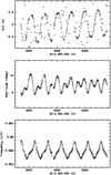 |
Fig. 9. Same as Fig. 7 except for synthetic data as described in Sect. 3.3.2. |
| In the text | |
|
Fig. 10. Top left panel: power spectrum of SMEI observations between frequencies f1 and f3 (Table 5). Top right panel: as top left, except for combined SMEI and BRITE data. Other four panels: power spectra of a single sine function with frequency f2 evaluated at SMEI observing times. This variation is modulated with different amplitudes (A) and frequencies (F). 0.0003125 c/d is about the inverse of the time span of the SMEI observations. Middle left panel: A = 10 km s−1, F = 0.0003125 c/d; there is almost no difference w.r.t. the SMEI observations. Middle right panel: A = 30 km s−1, F = 0.0003125 c/d; the strength of the side lobes increases with the amplitude. Bottom left panel: A = 20 km s−1, F = 0.0003125 c/d; bottom right panel: A = 20 km s−1, F = 0.000625 c/d. The separation of main peak and side lobes increases with modulation frequency. |
| In the text | |
|
Fig. 11. Left panel: same as top left panel of Fig. 10 except for compressed abscissa. Right panel: same as lower four panels of Fig. 10 except for compressed abscissa and A = 12 km s−1 and F = 0.0057 c/d, corresponding to a 1-M⊙-star orbiting ν Pup at 1 au. In the left panel, f1–f3 (Table 5) are visible whereas the synthetic data in the right panel only include f2 and its side lobes due to the assumed orbital motion. |
| In the text | |
|
Fig. 12. Cross-correlation functions between the two IUE observations of ν Pup and the 45 kK model template as described in Sect. 3.5. Because of different degrees of similarity to the spectrum of the Be primary, the cross-correlation functions for the 45 kK template are narrower than those with the 35 kK and 27.5 kK templates. The horizontal line indicates a signal-to-noise ratio level of 3.0 above which a companion with temperature ∼45 kK would be considered significant. |
| In the text | |
Current usage metrics show cumulative count of Article Views (full-text article views including HTML views, PDF and ePub downloads, according to the available data) and Abstracts Views on Vision4Press platform.
Data correspond to usage on the plateform after 2015. The current usage metrics is available 48-96 hours after online publication and is updated daily on week days.
Initial download of the metrics may take a while.