| Issue |
A&A
Volume 620, December 2018
|
|
|---|---|---|
| Article Number | A142 | |
| Number of page(s) | 20 | |
| Section | Planets and planetary systems | |
| DOI | https://doi.org/10.1051/0004-6361/201833691 | |
| Published online | 10 December 2018 | |
Deciphering the atmosphere of HAT-P-12b: solving discrepant results★
1
Leibniz-Institut für Astrophysik Potsdam (AIP),
An der Sternwarte 16,
14482 Potsdam,
Germany
e-mail: xalexoudi@aip.de
2
Stellar Astrophysics Centre (SAC), Department of Physics and Astronomy, Aarhus University,
Ny Munkegade 120,
8000 Aarhus C, Denmark
3
Department of Astronomy, University of Virginia,
Charlottesville,
VA 22904, USA
4
Astrophysics Group, Keele University,
Staffordshire,
ST5 5BG, UK
5
Dipartimento di Fisica, Università di Roma Tor Vergata,
Via della Ricerca Scientifica 1,
00133 Rome, Italy
6
Max Planck Institute for Astronomy,
Königstuhl 17,
69117 Heidelberg, Germany
7
INAF - Osservatorio Astrofisico di Torino,
Via Osservatorio 20,
10025 Pino Torinese, Italy
8
Department of Astronomy, Stockholm University, Alba Nova University Center,
106 91
Stockholm, Sweden
Received:
21
June
2018
Accepted:
3
October
2018
Context. Two independent investigations of the atmosphere of the hot Jupiter HAT-P-12b by two different groups resulted in discrepant solutions. Using broad-band photometry from the ground, one study found a flat and featureless transmission spectrum that was interpreted as gray absorption by dense cloud coverage. The second study made use of Hubble Space Telescope (HST) observations and found Rayleigh scattering at optical wavelengths caused by haze.
Aims. The main purpose of this work is to determine the source of this inconsistency and provide feedback to prevent similar discrepancies in future analyses of other exoplanetary atmospheres.
Methods. We studied the observed discrepancy via two methods. With further broad-band observations in the optical wavelength regions, we strengthened the previous measurements in precision, and with a homogeneous reanalysis of the published data, we were able to assess the systematic errors and the independent analyses of the two different groups.
Results. Repeating the analysis steps of both works, we found that deviating values for the orbital parameters are the reason for the aforementioned discrepancy. Our work showed a degeneracy of the planetary spectral slope with these parameters. In a homogeneous reanalysis of all data, the two literature data sets and the new observations converge to a consistent transmission spectrum, showing a low-amplitude spectral slope and a tentative detection of potassium absorption.
Key words: planets and satellites: gaseous planets / planets and satellites: atmospheres / stars: individual: HAT-P-12
The transit light curves of HAT-P-12b are only available at the CDS via anonymous ftp to cdsarc.u-strasbg.fr (130.79.128.5) or via http://cdsarc.u-strasbg.fr/viz-bin/qcat?J/A+A/620/A142
© ESO 2018
1 Introduction
In the past years, the field of exoplanetary sciences has been enriched by the numerous missions dedicated to the discovery and characterization of the planets beyond our solar system. Since the breakthrough of the first exoplanet orbiting a main-sequence star (Mayor & Queloz 1995), we can count up to almost 4.000 exoplanets by mid-20181.
Many methods are used for the detection of planets outside our solar system. The most prevalent of them is the observation of transits. The term “transit” is used to define the passage of the planet in front of its host star, which for a moment blocks a portion of the transmitted starlight. The received radiation is diminished by an amount equal to the ratio between the disk sizes of the planet and the host star. Granted sufficient observational cadence and photometric precision, this method provides precise estimates of the planetary and orbital parameters (period, radius ratio, inclination, etc.).
Transmission spectroscopy is one of the advantages that the transit observations can offer. This technique is considered a fundamental tool for characterizing exoplanetary atmospheres (Charbonneau et al. 2002). During the transit, part of the starlight is filtered as it passes through the upper atmosphere of the planet, where the atoms and molecules can absorb or scatter accordingly, revealing the elemental composition of an exoplanetary atmosphere (Burrows 2014; Madhusudhan et al. 2016; Deming & Seager 2017). The most suitable targets for transmission spectroscopy are hot Jupiters, which orbit their host star at very close distances. The studies of this specific group of exoplanets have so far revealed a tremendous diversity of planetary atmospheres: from clear atmospheres to those that are cloudy and dominated by haze (e.g., Sing et al. 2016; Lendl et al. 2016; Wakeford et al. 2017; Mallonn & Wakeford 2017; Tsiaras et al. 2018; Kreidberg et al. 2018; Nikolov et al. 2018).
The characterization of an exoplanetary atmosphere requires a very careful analysis because the signal of the planetary atmosphere is at most about 0.1% of the stellar flux (Deming & Seager 2017). The exoplanet community succeeded in providing robust results that were confirmed by independent teams. Examples are the clear atmosphere of WASP-39b (Fischer et al. 2016; Sing et al. 2016; Nikolov et al. 2016), the hazy atmosphere of GJ3470b (Nascimbeni et al. 2013; Dragomir et al. 2015; Chen et al. 2017), and the flat transmission spectrum for GJ1214b (Berta et al. 2012; Kreidberg et al. 2014; Nascimbeni et al. 2015). However, since this research takes place at the edge of what can be detected, contradicting results regarding individual planets are reported in the literature as well. Potential reasons may be the different and underestimated systematic errors, the various assumptions in the analysis (e.g., different limb-darkening laws, LDLs), or even the time variability of the atmosphere. Examples of deviating results are the quest for potassium absorption in WASP-31b (Sing et al. 2015; Gibson et al. 2017) and the debates on the spectral slope of WASP-80b (Sedaghati et al. 2017; Kirk et al. 2018; Parviainen et al. 2018) and TrES-3b (Parviainen et al. 2016; Mackebrandt et al. 2017).
A specific example for a controversy in atmospheric characterization is the sub-Saturn HAT-P-12b (Hartman et al. 2009). Previous studies on the atmosphere of this exoplanet by two different groups have shown significant deviations. The first study, Mallonn et al. (2015), hereafter M15, used ground-based broad-band photometry observations and derived a flat transmission spectrum, indicating an opaque layer of clouds as an atmospheric scenario for HAT-P-12b. The second study, carried out by Sing et al. (2016), hereafter S16, used HST spectroscopy observations and found astrong Rayleigh-scattering signature at optical wavelengths that is indicative of a haze layer. The transmission spectra of both works are presented in Fig. 1, with the discrepancy being evident at short wavelengths.
The goal of our work is to investigate the cause of this inconsistency regarding HAT-P-12b. The previous studies differ in several details of the analysis. Different fit routines were used, and with the aim to account for the effect of stellar limb darkening, different laws were employed by the two groups. More specifically, M15 fit the light curves with a quadratic LDL, with coefficients obtained from Claret & Bloemen (2011). S16 adopted the four-parameter LDL (Claret 2004) and calculated new coefficients. Both studies also made different assumptions about the orbital parameters. The effect of these different assumptions on the analyses is determined and cautiously investigated in this work. We attempt to resolve the discrepancy with a homogeneous reanalysis of all the existing data sets. Moreover, in order to increase the precision at bluer wavelengths, where the discrepancy is more pronounced, we obtained additional, new transit observations.
This work is organized as follows. In Sect. 2, we present the new transit observations of HAT-P-12b from different facilities from the ground. In Sect.3, we briefly describe the data reduction. In Sect. 4, we fully explain the method for the light-curve analysis and for the estimation of the error bars. In Sect. 5, we present the results of this work, and we identify the likely source of the inconsistency regarding HAT-P-12b as the degeneracy between the inclination and the optical spectral slope. We include a homogeneous reanalysis of the available data. In Sect. 6, we discuss our results and conclude with a final atmospheric characterization for this exoplanet.
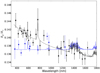 |
Fig. 1 Published transmission spectra of HAT-P-12b. The measurements of the planet-star radius ratio Rp∕R⋆ over wavelength are presented for both works. The results of M15 are shown with blue squares, and the measurements of S16 are shown with black diamonds. Two models of Fortney et al. (2010) are overplotted and present atmospheres that are dominated by clouds (blue line) and haze (black line). |
2 Data acquisition
In order to investigate the disagreement published in the literature for the atmospheric characterization of HAT-P-12b, we collected the existing data obtained with ground-based observations (M15) and with the HST (S16), with the aim to perform the analysis of the two different groups step by step in a homogeneous way. Additionally, we obtained data of ten new primary transit events in 2016–2017 in Johnson B and Sloan g′ filters with different facilities. Using selected broad-band filters, meter-class telescopes are able to provide sufficient accuracy to reveal general trends in a transmission spectrum, for instance, a scattering optical slope (Dragomir et al. 2015; Mallonn et al. 2016; Mackebrandt et al. 2017).
2.1 Published data set of M15
The data sample of M15 included newly observed transit light curves complemented by light curves from the publications of Hartman et al. (2009), Sada et al. (2012), and Lee et al. (2012). These data spanned the time range of 2007 to 2014, the wavelength range from Sloan u′ band to J band in ten different filters, and were observed with ground-based 1-m telescopes such as STELLA, medium-class telescopes such as the Telescopio Nazionale Galileo (TNG), and telescopes with mirrors of up to 8 m such as the Large Binocular Telescope. In this work, we reanalyze the light curves from Sloan u′ band to Sloan z′ band and exclude partial transits. This sample of ground-based literature light curves is furthermore extended by one light curve of Turner et al. (2017) that was obtained in the Johnson B band with the 1.5-m Kuiper Telescope.
2.2 Published data set of S16
The space-based data of HAT-P-12b, provided by S16, are a part of a comparative study of ten hot Jupiters (Program GO-12473, PI: D.K. Sing). HAT-P-12b was observed in the full optical wavelength range from 0.3 to 1.01 μm with the Space Telescope Imaging Spectrograph (STIS, Woodgate et al. 1997). Additionally, for observations in the near-infrared, the Wide Field Camera 3 (WFC3, Leckrone et al. 1998) was also used, and the Spitzer Space Telescope Infrared Array Camera (IRAC, Fazio et al. 2004) completed this survey with observations at 3.6 and 4.5 μm. Observations of two transits of HAT-P-12b were performed with the STIS G430L grating, covering the wavelengths from 0.29 to 0.57 μm (visit 11 and visit 12), and one observation with the G750L grating, covering the range from 0.524 to 1.027 μm (visit 22).
The team of S16 provided us with the reduced HST/STIS light curves. The visits were scheduled so that the transit is shown at the third spacecraft orbit, whereas the out-of-transit baseline is contained in the first, second, and fourth orbits. Each visit consists of four telescope orbits of 96 min. The gaps are due to the stellar target’s occultation by the Earth. A total of 24 spectroscopic light curves were acquired during the three visits (visit 11: seven light curves, visit 12: seven light curves and visit 22:ten light curves). The data were bias-, flat-field- and dark-corrected using the latest version of CALSTIS following a procedure described fully in Nikolov et al. (2015).
2.3 New observations
We obtained new transit light curves in 2016 and 2017 from five ground-based facilities, which are the 3.5-m TNG on the Roque de los Muchachos Observatory, the 1.23-m and 2.2-m telescopes of Calar Alto Observatory, the 3.5-m Astrophysics Research Consortium (ARC) telescope from Apache Point Observatory, and the 1.2-m STELLar Activity (STELLA) telescope (Strassmeier et al. 2004).
2.3.1 ARC observations
HAT-P-12b was observed during the night of 5 July 2017 with the ARCTIC instrument (Huehnerhoff et al. 2016) on the 3.5-m ARC telescope, Apache Point Observatory (program UV04, PI: J.D. Turner). ARCTIC was employed in imaging mode using the J-C B filter, and a binning of 2 × 2 pixels gave a plate scale of 0.228′′ pixel−1. The fast mode yielded a readout time of 11 s with an exposure of 45 s.
2.3.2 TNG observations
One transit of HAT-P-12b was observed during the night of 18 May 2017 using the DOLORES instrument (Oliva 2006) on TNG with a Johnson B filter (Director’s Discretionary Time (DDT) program A35DDT2, PI: X. Alexoudi). With 40 s of exposure time, we achieved a signal-to-noise ratio (S/N) per exposure of approximately 1800. Taking into account the read-out time (25 s) and the image transfer time (6 s), we achieved a 71-s cadence that corresponds to a duty cycle of 56%. We defocused the telescope on purpose to about 4′′ full width at half-maximum (FWHM) of the object point-spread function (PSF) to avoid saturation of the detector. No windowing was applied, and the field of view (FOV) was 8.6′ × 8.6′.
2.3.3 CALAR ALTO 2.2m observations
On 18 May 2017, we were also awarded with DDT (Program DDT.S17.166, PI: X. Alexoudi) to observe with the Calar Alto 2.2-m telescope with CAFOS (Meisenheimer 1994). We used the Johnson B filter with an exposure time of 60 s. With a binning of 2 × 2 pixels and an appropriate windowing of the region of interest, we concluded to a cadence of approximately 80 s and therefore a duty cycle of 73%. The telescope was again defocused to about 4′′ FWHM to avoid saturation of the detector.
2.3.4 Calar Alto 1.23m observations
Two complete transit events of HAT-P-12b were observed between March and May 2017 using the Zeiss 1.23-m telescope, which is equipped with the DLRMKIII (Barrado et al. 2011) camera (4000 × 4000 pixels of 15 μm size) and has an FOV of 21.5′ × 21.5′. The two transits were observed using a Johnson B filter and adopting the defocussing technique for using longer exposure times (120–150 s). This significantly improved the quality of the photometric data. The telescope was autoguided, and the CCD was windowed to decrease the readout time.
2.3.5 STELLA observations
In total, five transit observations of HAT-P-12b were obtained with STELLA with a Sloan g′ filter in 2016 and 2017. All observations were defocused to about 3′′ FWHM for the PSF. We reduced the available FOV of 22′ × 22′ by a read-out window of about 15′ × 15′ to shorten the readout time.
3 Data reduction of ground-based data
The data reduction of the majority of the new observations was carried out using a customized ESO-MIDAS pipeline, which deploys the photometry software SExtractor (Bertin & Arnouts 1996). The procedure is fully described in previous works of Mallonn et al. (2015, 2016). The only exception was the ARC observation, which was reduced using the softwaredescribed in Turner et al. (2016) and Pearson et al. (2014). Table 1 shows the new observations as obtained from the different facilities in detail. The light curves were acquired with Johnson B and Sloan g′ filters (Figs. 2 and 3). The rms scattering of the residuals in most cases is less than 2 mmag. The correlated noise measured with the β factor (see Sect. 4.1) is close to unity in the majority of our time series.
4 Data analysis
4.1 Treatment of photometric errors
A realistic assessment of the individual photometric error bars of the transit light curves is mandatory to finally derive realistic uncertainties on the transit parameters. We derived photometric uncertainties, based on the assumption of white noise, from the photometry software SExtractor (Bertin & Arnouts 1996) as regular part of the data reduction. These uncertainties yield a  larger than unity when an initial transit model was fit. This is an indicator that the individual photometric error bars are underestimated. Therefore, we enlarged the photometric error bars by a factor that forces
  . The obtained light curves often suffer from correlated (red) noise, in addition to the photon noise. The red noise is produced by a combination of systematic errors, such as changes in the atmospheric conditions, tracking of the telescope, or relative flat-field errors. Thus, adjacent points of a light curve become correlated (Pont et al. 2006). This kind of correlated noise leads to underestimated errors of the transit parameters and inconsistent parameterization of the light curves. To quantify the influence of red noise in our data, we used the concept of “β factor” (Winn et al. 2008):
 (1)
(1)
where σr is the standard deviation of the binned residuals into M bins of N points, and σN is the expected standard deviation according to
 (2)
(2)
where σ1 is the standard deviation of the unbinned residuals. In absence of correlated noise, β equals unity. In the presence of correlated noise, the standard deviation of the binned data is different by a factor β from the theoretically expected one (von Essen et al. 2013). The β value depends on the bin size. Therefore, we binned the residual light curves using ten binning widths of 0.3–1.3 times the duration of ingress. The final β value is the average of these ten individual values. Because of statistical fluctuations, the β value might sometimes be lower than 1. For these cases, we set β = 1 as a default. Finally, we enlarged the individual photometric error bars by the corresponding amount of β for all ground-based new and literature light curves.
The HST/STIS light curves show too few data points per orbit to reasonably apply the method of the binned residuals, therefore we adopted β = 1 for the HST data. The photometric noise was verified to yield a  .
.
Overview of the new observations of transits of HAT-P-12b during 2016 and 2017.
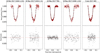 |
Fig. 2 Newly obtained B band light curves of the transit event of HAT-P-12b (upper panels). The light curves are fit and detrended according to the description of the homogeneous reanalysis in Sect. 5.3. Associated residuals of each light curve (lower panels). |
4.2 Light-curve fitting
4.2.1 Transit modeling
We made use of the Python library PyAstronomy2, which is a collection of packages related to astronomy developed by the PyA team at the Hamburger Sternwarte. The PyAstronomy packages contain the analytical transit model formulae of Mandel & Agol (2002) and a class that allows for multiple light-curve fitting in a simultaneous way. The model of Mandel & Agol (2002) is validated for light-curve modeling with the main advantage that it is capable, when used in a fitting procedure, to extract the most suitable system parameters and to investigate their possible correlations. This model is appropriate for systems with a circular or Keplerian orbit. It considers the planet and the star as spheres, while the effect of the limb darkening isalso taken into account by using either the quadratic or the four-parameter LDLs. For HAT-P-12b, we adopted a circular orbit for the system, as derived from radial velocity (RV) data and reported in Hartman et al. (2009) and Knutson et al. (2014). The parameters that constructed the model were the orbital period P, the semi-major axis in units of stellar radius a∕R⋆, the inclination of the system i, the radius of the planet over the radius of the star k = Rp∕R⋆, the limb-darkening coefficients, and the time of the mid-transit T0. The initial values for these parameters were adopted from the literature, from the works of Hartman et al. (2009) and M15. We used the ephemeris given in M15. Throughout this work, we employ a Markov chain Monte Carlo (MCMC) fitting approach, enabled by PyAstronomy. Each fit consists of 300 000 MCMC iterations, rejecting the first 50 000 samples as burn-in phase, ensuring that the final sample is extracted from a well-converged MCMC chain, where the deviance is minimized yielding the best-fit solution. To examine the variety of probable solutions for each free-to-fit parameter, we assumed conservatively uniform prior probability distributions. In the next step, we analyzed the posterior distributions of each parameter and obtained the mean values along with their standard deviations. The errors given throughout this work correspond to 68.3% highest probability density (HPD) intervals of the posterior probability distributions of each parameter, denoting the 1σ level. We checked for convergence of the chains by splitting them into three equally sized sub-groups and verified that their individual mean agreed within 1σ.
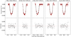 |
Fig. 3 Newlyobtained g′ band light curves (upper panels), fit and detrended as described in Sect. 5.3 (similar to Fig. 2). Their residuals are shown in the lower panels. |
4.2.2 Detrending model for the ground-based data
The physical properties of the observations, such as airmass, time, seeing, and x and y drifts of the pixel position, were used in different combinations to build up a variety of detrending models, as suggested by von Essen et al. (2016). They were fit simultaneously to the transit model. The choice of the best detrending function can be determined by the Bayesian information criterion (BIC, Schwarz 1978):
 (3)
(3)
where k is the number of model parameters, N the number of data points, and χ2 is the chi-squared statistic. The value of χ2 is calculatedas
 (4)
(4)
where Obsi refers to the observed data points and Modi to the fit model, erri are the photometric error bars, and n denotes the total number of data points. By testing many combinations of detrending functions on our light curves, we concluded that a light-curve model M(t) including a second-order time-dependent polynomial
![\begin{equation*}M(t)\,=\,M_0(t)\,[\mathrm{\textit{b}_0} + \mathrm{\textit{b}_1} t + \mathrm{\textit{b}_2} t^2],\end{equation*}](/articles/aa/full_html/2018/12/aa33691-18/aa33691-18-eq8.png) (5)
(5)
where M0(t) is the model for a systematics-free transit model described in Sect. 4.2.1, and b0, b1 and b2 denote the coefficients of the parabola over time, is more efficient, as it minimizes the BIC value for the vast majority of ground-based light curves. This finding is in agreement with M15 in the specific case of HAT-P-12b and with numerous studies on photometric transit light curves obtained with small-size telescopes in general (e.g., Biddle et al. 2014; Maciejewski et al. 2015; Mancini et al. 2016; Mackebrandt et al. 2017; Juvan et al. 2018).
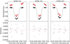 |
Fig. 4 White-light curve fitting for the HST data. The red dots show the raw data, and overplotted with the red solid line, we show the transit model according to the homogeneous reanalysis in Sect. 5.3. The black dots and black solid line indicate the detrended light curves. Lower panels: associated residuals. |
4.2.3 Detrending model for the HST data
The systematics model for HST data is different in comparison to the analysis of the ground-based data. We employed a model similar to the work of Huitson et al. (2013), Nikolov et al. (2014), and S16. In this model, we need to take into account the flux corrections for each orbit with the fitting of a fourth-order polynomial of the orbital phase ϕ of the HST. Higher (fifth- and sixth-) order polynomials are in general not suggested for parameters in a detrending model because they result in larger BIC numbers (Nikolov et al. 2014). Moreover, our detrending model takes into account the shift of the detector positions x and y. Huitson et al. (2013) reported that linearlyfitting the x- and y- offsets of the spectra results in a smaller BIC and a better fit. Furthermore, our systematics model needs to account for the out-of-transit baseline with the use of an offset q0 and a linear term q1, dependent on time. In the end, the final systematic to consider is the spectral shift sh in the dispersion direction. During an observation, the spectrum does not remain at the same place, and for this reason, a pixel does not receive the same wavelength for each exposure. This creates response variations from one exposure to another. Using the cross-correlation technique with the initial first exposure spectrum, S16 determined that this spectral shift is not negligible. Therefore, the complete systematics model we used for the detrending is
![\begin{eqnarray*} M(t)\,& = &\,M_0(t)\,[\mathrm{\textit{q}_0} + \mathrm{\textit{q}_1} t+ \mathrm{\textit{q}_2}\phi + \mathrm{\textit{q}_3}\phi^2 + \mathrm{\textit{q}_4}\phi^3 + \mathrm{\textit{q}_5}\phi^4 \nonumber \\ & & +\,\mathrm{\textit{q}_6} sh\,+\, \mathrm{\textit{q}_7} x\,+\, \mathrm{\textit{q}_8} y],\end{eqnarray*}](/articles/aa/full_html/2018/12/aa33691-18/aa33691-18-eq9.png) (6)
(6)
with q0–q8, the coefficients of each term. The systematics model can be also multiplicative rather than additive (Sing 2018). As suggested by previous studies with STIS (Huitson et al. 2013), we neglected the first orbit measurements to avoid higher systematic errors. These systematics are usually caused by the telescope heating and cooling per orbit, a term known as “thermal breathing”. The temperature changes because of the expansion or contraction of the telescope, thus these are interpreted as variations in the central position of the spectrum and in the PSF. Because of these problems with the first exposure of each orbit (Sing et al. 2011), we neglected these individual data as well. Figure 4 shows the white-light curves of the three visits overplotted with our transit and detrending model.
5 Results
5.1 Reanalysis of the ground-based data
Our ground-based data set consisted of photometric transit light curves from M15 (Hartman et al. 2009; Sada et al. 2012; Lee et al. 2012), 1 light curve from Turner et al. (2017), and our 10 new light curves of Table 1. We made use of a total number of 35 light curves that were observed during a time period covering ten years (2007–2017).
As the first step of our analysis, we attempted to reproduce the broad-band filter transmission spectrum of M15. For this purpose, we adapted the details of the analysis of this work, which employs the quadratic LDL with the two coefficients u and v. The latter was fixed to the theoretical values provided in M15, while the former was left free to fit. The transit parameters T0, a∕R⋆, i, and P were fixed to the values of M15. The model fit consisted of the following free-to-fit parameters: one value per broad-band filter of k and u, along with the three constants b0, b1, and b2 of the time-dependent polynomial (Eq. (5)) per individual light curve. The reanalyzed detrended light curves are presented inFigs. 2, 3, and A.3–A.9. From this global fit and frominvestigating the credibility intervals of the parameters, we find compatible results with M15 for k over wavelength, as shown in Fig. 5.
To conclude this part of our work, using the same LDL and applying the same treatment of the fit parameters, using the same detrending model and the same enlargement procedure on the photometricerrors, but another fitting routine, we were able to reproduce the results obtained by M15. It is important to emphasize that our work includes additional light curves from new observations in Johnson B and Sloan g′ filters, obtained with different facilities from the ground, which improved our precision in both bands. The broad-band results agree with aflat transmission spectrum of HAT-P-12b within one atmospheric pressure scale height. However, the discrepancy concerning the atmosphere of HAT-P-12b is not yet understood. Therefore, we will continue this investigation by taking into account the different LDLs deployed by the different groups and the different system parameters used for the light-curve analyses.
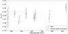 |
Fig. 5 Reanalysis of the ground-based data of HAT-P-12b and comparison with the previous results from M15. The values of this work are offset in wavelength for better visibility. We included additional data for the B and g′ band data at 435 and 475 nm, which results in higher precision. |
Transit parameters of HAT-P-12b derived in this work and comparison to previously published values.
5.1.1 Importance of the LDLs
The studies of M15 and S16 differ in the choice of the LDL. While the former uses the quadratic law, the latter employs the four-parameter LDL with its coefficients α1, α2, α3, and α4. To investigate the importance of this choice in the case of HAT-P-12b, we employed both the quadratic and the four-parameter LDL by fitting the ground-based data again. We used the coefficients provided by Claret & Bloemen (2011) from stellar ATLAS models. We also investigated a plausible change in k when fixing all coefficients to theoretical values in comparison to leaving the first coefficient of either the quadratic or of the four-parameter LDL free to fit.
For all cases, the difference in k is not significant. The values per individual filter change only by a fraction of our 1σ uncertainties, whereas the overall slope remains unaffected.
Moreover, to investigate the suggestion by Csizmadia et al. (2013) that different theoretical calculations of the limb-darkening coefficients by individual authors might lead to varying results for k, we fit our light curves with limb-darkening coefficients obtained from both S16 and Claret & Bloemen (2011). However, the effect of the coefficients from different authors is not of significance either. The obtained k per filter is in agreement with the published ground-based data of HAT-P-12b and supports a flat-spectrum scenario at optical wavelengths.
The main outcome of this part of the analysis is that different LDLs and coefficients are certainly not the cause of the discrepancy in the published transmission spectra of HAT-P-12b. In a further step toward the clarification of the problem, we investigated the effect of the orbital parameters on the light-curve fitting procedure, and specifically, the influence of the system inclination.
5.1.2 Importance of the system inclination
Both studies, M15 and S16, fixed the orbital parameters i and a∕R⋆ when they fit for k over wavelength. The one work fixed these parameters to values that they derived from a joint fit to all their data, the other work fixed these parameters to values derived from the HAT-P-12b Spitzer light curves of S16. In this section, we investigate the effect of these parameters on the value of k using the example of i. The literature agrees (Table 2) on an inclination value for the HAT-P-12 system of about 89° (Hartman et al. 2009; Line et al. 2013; Mallonn et al. 2015; Mancini et al. 2018). We defined three cases in total with fixed different inclinations of 88°, 89°, and 90°. We chose the four-parameter LDL with fixed coefficients (Claret & Bloemen 2011) and fit the ground-based light curves again with the aim to investigate if there is a significant variation in k with respect to i. Figure 6 shows that changes in the fixed inclination value cause an offset in k, which is wavelength dependent. Therefore, a change in i can cause a slope in the transmission spectrum. Potentially, the assumption of an inaccurately small inclination for HAT-P-12b could imply a Rayleigh slope.
This dependency of the optical slope on the orbital parameters is briefly described in Pont et al. (2013). With our investigation, we verify that the discrepancy between M15 and S16 is potentially based on this degeneracy of i and k. By a joint fit of all ground-based light curves with free transit parameters i, a∕R⋆, and k, we derive a refined value for the inclination, i = 88.83° ± 0.19°.
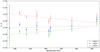 |
Fig. 6 Variation in transmission spectrum for three different inclination values. Different values of i cause an offset in k, which is wavelength dependent. This effect can mimic a slope in the transmission spectrum. The dashed lines mark linear regressions. |
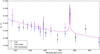 |
Fig. 7 Reanalysis of the HST data using the orbital parameters derived by S16 using the Spitzer transit light-curves. The reproduced transmission spectrum (blue data points) agrees well with the transmission spectrum of S16 (magenta points). |
5.2 Reanalysis of the HST data
In this part of our work, we test if the sloped HST/STIS transmission spectrum can be reproduced, following the analysis procedure described in S16 step by step. Because the HST light curves lack observational data during transit ingress and egress, they are not suited to accurately constrain the orbital parameters i and a∕R⋆. Therefore, S16 derived these parameters from the two Spitzer light curves at 3.5 and 4.6 μm included in their work, resulting in iS16 = 88.10° ± 0.27 and a∕R⋆,S16 = 11.19 ± 0.22 (Nikolov, priv. comm.).
We derived the STIS transmission spectrum from the set of light curves over wavelengths as supplied to us by the team of S16, keeping i and a∕R⋆ fixed to the Spitzer values. A detrending model similar to S16 was employed (see Sect. 4.2.3), and as carried out by S16, we used the four-parameter LDL with coefficients fixed to theoretical values. The free-to-fit parameters were k per wavelength channel and detrending coefficients per light curve. The detrended light curves are presented in Figs. A.1 and A.2.
Figure 7 shows the resulting reanalyzed transmission spectrum, which agrees very well with the spectrum presented in S16. We summarize that S16 suggested slightly different orbital parameters than were given by a fit to the numerous ground-based data and in the literature. If these parameter values are used to derive the transmission spectrum, we reproduce an evident slope of k over wavelength.
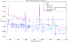 |
Fig. 8 Transmission spectrum of HAT-P-12b as derived from the homogeneous reanalysis of all data from the ground and from the HST with their associated error bars. For reference and comparison, we overplot the values obtained by M15 (black empty squares). The blue dashed lines show plus–minus two scale heights from the weighted average value of k (blue dotted line). In magenta we show the values of S16 together with the suggested atmospheric model (magenta solid line). The cyan solid overplotted line represents the cloud-free, solar-composition model of HAT-P-12bfrom Fortney et al. (2010) for comparison. The blue solid line is a linear regression of the weighted k values. |
5.3 Homogeneous reanalysis of all data
In the previous parts of this work, we successfully reproduced the published results from M15 and S16 with the analyses of each data set independently and according to the published procedure of each group. Now, we aim for a homogeneous reanalysis of both the ground-based and the space-based data. We consider the orbital parameter values derived in this work (Table 2) as the most accurate ones because they are drawn from a very large sample of independently observed data. The remaining systematic noise inherent to the individual light curves of this sample is expected to average out. Moreover, these values broadly agree with the literature values published previously, while the S16 values deviate by about 2 σ. The source of this slight deviation might be pure statistical fluctuation and is not investigated further here. Thus, we fixed i and a∕R⋆ to the best-fit ground-based values, and let k vary for in total 17 wavelength channels of the HST data and eight broad-band filters of the ground-based data. Each individual light curve has its own independent and simultaneously fit detrending function. The wavelength-dependent limb-darkening coefficients of the four-parameter LDL were fixed to the theoretical values from Claret & Bloemen (2011). The result, that is, the final transmission spectrum, is presented in Fig. 8 and Table 3. The k values of ground- and space-based data finally agree broadly.
5.4 Physical parameters and the ephemeris of HAT-P-12b
Based on our newly derived transit parameters, we refined the planetary properties using the equations from Southworth et al. (2007, 2010), Winn (2010), Seager (2011), and Turner et al. (2016):
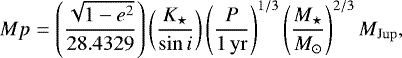 (7)
(7)
where K⋆ = 35.8 ± 1.9 km s−1 is the RV semi-amplitude of the star and M⋆ = 0.73 M⊙ (Hartman et al. 2009). M⊙ denotes one solar mass. The variable e stands for the eccentricity of the system, which in case of HAT-P-12b is assumed to be zero. The surface gravitational acceleration is
 (8)
(8)
and the modified equilibrium temperature Teq is given by
 (9)
(9)
where Teff is the effective temperature of the host star. The formula is derived under the assumption that A = 1 − 4F, with A the Bond albedo and F the heat redistribution factor (Southworth 2010).
The ability of the planet to interact with other bodies in its environment is measured by the Safronov number Θ (Safronov 1972):
 (10)
(10)
To refine the orbital ephemeris, we derived the individual mid-transit times of the new transit observations by a separated fit individually to every light curve, summarized in Table 4, and combined them with the published mid-transit times from Mallonn et al. (2015). A weighted linear least-squares fit to all the mid-transit times versus their cycle number resulted in an updated ephemeris:
 (11)
(11)
Here, Tc denotes the predicted transit central time and N the corresponding cycle number of the reference mid-time. The orbital period agrees with that published by Mallonn et al. (2015), with slightly improved precision, and it shows a difference of about 1 σ to the work of Hartman et al. (2009).
In Table 5, we compare our values with the most recent literature values of HAT-P-12b (Mancini et al. 2018), and our results are in agreement. Moreover, the equilibrium temperature estimated here agrees with the upper limit on the brightness temperature derived by Todorov et al. (2013) if for simplicity we assume the planet to radiate as a blackbody.
6 Discussion and conclusion
The motivation for this work was to draw a homogeneous picture of the atmosphere of HAT-P-12b and to solve the discrepancy between the transmission spectra published by M15 and S16. During the analysis, we found that this discrepancy was not caused by the different analysis tools, as M15 used Levenberg-Marquardt fitting with the JKTEBOP software package (Southworth 2008) and S16 used the MCMC fitting of the Mandel & Agol (2002) transit models. Neither was the usage of different LDLs the reason, nor could it be found in subtle differences in the treatment of the limb-darkening coefficients. Following the procedures of both studies for an individual reproduction of their results, we noted a difference in the orbital planetary parameters that is the likely cause of the discrepancy. While both teams assumed the parameters i and a∕R⋆ to be wavelength independent and kept them fixed during their final light-curve fit, they derived different values for them. The value of M15 agreed with previous literature values, while the light-curve fit of two Spitzer light curves of S16 yielded slightly deviating orbital parameters (Nikolov, priv. comm.). With these two sets of parameters, we succeeded in reproducing the deviating transmission spectrum. When we reanalyzed all ground-based and space-based data using newly derived values for the orbital parameters, we found consistent results among all observations. New transit light curves taken at short wavelengths increased the precision further.
HAT-P-12b is one of the ten targets of the comparative study of S16. The orbital parameters of the other targets, derived from the fit to HST white-light curves (Huitson et al. 2013; Sing et al. 2013, 2015; Nikolov et al. 2014, 2015), are generally in good agreement with previously published values. Therefore, HAT-P-12b probably is a particular case in the HST survey planet sample, and we currently find no indications that would make a reanalysis of other data of this sample necessary.
To our knowledge, a degeneracy between the orbital parameters i and a∕R⋆ and the derived slope in the exoplanet transmission spectrum is not thoroughly discussed in the literature. Such an exercise was not foreseen for this paper either, but an extensive work based on simulated data is currently prepared by our team. Many hot Jupiters that have been investigated with transmission spectroscopy show a (negative) slope in their spectrum, which is generally interpreted as a signature of scattering by aerosol (haze) particles (e.g., Jordán et al. 2013; Sing et al. 2016; Mallonn & Wakeford 2017; Chen et al. 2017). It is extensively discussed in literature that such a slopecan also be mimicked by third light of another stellar body falling to the photometric aperture and brightness inhomogeneities such as spots and faculae on the host star photosphere (Oshagh et al. 2014; Rackham et al. 2018; Mallonn et al. 2018). Without a proper knowledge of all factors that potentially influence the measured slopes in exoplanettransmission spectra, a correct scientific interpretation is not possible. In this article, we wish to direct the attention of observers to a degeneracy of the orbital parameters with the optical exoplanet spectral slope.
The transmission spectrum of HAT-P-12b finally derived in this work has the best currently achievable precision. The data points shortward of 700 nm show a standard deviation of about 0.6 atmospheric pressure scale heights (H) with a mean uncertainty of about 0.8 H, including the less precise data points shortward of 400 nm. This is remarkable considering that the host star is comparably faint, with a V -band magnitude of 12.8, and that it is a K-type star with rather little stellar flux at short wavelengths. Our transmission spectrum is inconsistent with the clear-atmosphere, solar-composition model by Fortney et al. (2010), scaled to the parameters of this planet (Fig. 8). There is no indication for absorption by sodium in either an HST wavelength channel centered at the line core or at the wavelength of pressure-broadened wings, as predicted by the Fortney et al. (2010) model. The transmission data longward of 700 nm are less precise with larger uncertainties and larger scatter among the data points. These data did not show a significant indication for a pressure-broadened potassium line but they could not rule it out either. We agree with the finding by S16 of a tentative absorption signal in the core of the potassium line, but it is just significant at the 2 σ confidence level and based on only one single light-curve. Further observations are required to confirm this.
A linear regression line calculated using all our data points shows a slope of − 2.96 ± 1.28 × 10⁻⁶ nm−1. We consider this slope to be a signature of the planetary atmosphere because of the low activity level of the host star (Mallonn et al. 2015; Mancini et al. 2018). In units of H, this slope corresponds to a difference of about 1.5 H from the u′ band to the z′ band. With this amplitude, the spectral slope is rather typical for hot Jupiters (Sing et al. 2016; Mallonn & Wakeford 2017; Pinhas & Madhusudhan 2017). HAT-P-12b has an equilibrium temperature of 950 K (Sect. 5.4), thus, it is the coolest object of the ten planets in the HST survey. However, no dependence of the slope amplitude on temperature becomes evident, as HAT-P-12b has a very similar slope to 1100 K WASP-39b, 1450 K HD209458b, and even 2500 K WASP-12b (Sing et al. 2016; Mallonn & Wakeford 2017). HAT-P-12b is similar in equilibrium temperature and surface gravity to WASP-39b. However, the former presents an optical spectrum that is dominated by haze particles scattering, while the latter shows a rather clear atmosphere that reveals the pressure-broadened wings of sodium (Fischer et al. 2016; Wakeford et al. 2018). Future work may reveal whether this diversity is linked to differences in cloud condensation by different planetary metallicity abundances or planetary atmospheric dynamics. Another possibility may be differences in the production of photochemical haze by the different host star spectral types of HAT-P-12 and WASP-39.
Individual transit mid-times of the new transit observations of this work.
Estimates of the physical properties of HAT-P-12b as derived from this work in comparison to literature values recently provided by Mancini et al. (2018).
Acknowledgements
We thank the anonymous referee for the insightful comments. We thank Nikolay Nikolov and David Sing for discussions and comments on the manuscript. We are grateful to Jonathan Fortney for providing atmospheric models for HAT-P-12b, and we thank Antonio Claret for providing limb-darkening coefficients of HAT-P-12. We are grateful for DDT observing time at Calar Alto and wish to acknowledge all technical support at the involved observing facilities. L.M. acknowledges support from the Italian Minister of Instruction, University and Research (MIUR) through FFABR 2017 fund. L.M. acknowledges support from the University of Rome Tor Vergata through “Mission: Sustainability 2016” fund. This research has made use of the SIMBAD data base and VizieR catalog access tool, operated at CDS, Strasbourg, France, and of the NASA Astrophysics Data System (ADS). This work is partly based on data obtained with the STELLA robotic telescopes in Tenerife, an AIP facility jointly operated by AIP and IAC, partly based on observations made with the Italian Telescopio Nazionale Galileo (TNG) operated on the island of La Palma by the Fundación Galileo Galilei of the INAF (Istituto Nazionale di Astrofisica) at the Spanish Observatorio del Roque de los Muchachos of the Instituto de Astrofisica de Canarias, partly based on observations collected at the German-Spanish Astronomical Center, Calar Alto, jointly operated by the Max-Planck-Institut für Astronomie Heidelberg and the Instituto de Astrofísica de Andalucía (CSIC), and partly based on observations obtained with the Apache Point Observatory 3.5-m telescope, which is owned and operated by the Astrophysical Research Consortium.
Appendix A Additional figures
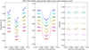 |
Fig. A.1 Raw light curves of HST visit 11 (left panel) and detrended light curves (middle panel). Overplotted are the fitted models of the homogeneous analysis of Sect. 5.3. The associated residuals are presented in the right panel. The curves are shifted arbitrarily for clarity. |
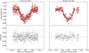 |
Fig. A.3 Reanalyzed, detrended literature u′-band light curves with the associated transit model described in Sect. 5.3. Bottom panels: associated residuals. |
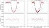 |
Fig. A.4 Reanalyzed, detrended literature B-band light curves with the associated transit model described in Sect. 5.3. Bottom panels: associated residuals. |
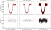 |
Fig. A.5 Reanalyzed, detrended literature g′-band light curves with the associated transit model described in Sect. 5.3. Bottom panels: associated residuals. |
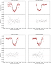 |
Fig. A.6 Reanalyzed, detrended literature V -band light curves with the associated transit model described in Sect. 5.3. Bottom panels: associated residuals. |
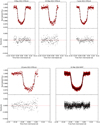 |
Fig. A.7 Reanalyzed, detrended literature r′-band light curves with the associated transit model described in Sect. 5.3. Bottom panels: associated residuals. |
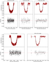 |
Fig. A.8 Reanalyzed, detrended literature R-band light curves with the associated transit model described in Sect. 5.3. Bottom panels: associated residuals. |
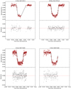 |
Fig. A.9 Reanalyzed, detrended literature two i′-band (upper panels) and two z′-band (lower panels) light curves with the associated transit model described in Sect. 5.3. Bottom panels: associated residuals. |
References
- Barrado, D., Thiele, U., Aceituno, J., et al. 2011, in Highlights of Spanish Astrophysics VI, eds. M. R. Zapatero Osorio, J. Gorgas, J. Maíz Apellániz, J. R. Pardo, & A. Gil de Paz, 637 [Google Scholar]
- Berta, Z. K., Charbonneau, D., Désert, J.-M., et al. 2012, ApJ, 747, 35 [NASA ADS] [CrossRef] [Google Scholar]
- Bertin, E., & Arnouts, S. 1996, A&AS, 117, 393 [NASA ADS] [CrossRef] [EDP Sciences] [Google Scholar]
- Biddle, L. I., Pearson, K. A., Crossfield, I. J. M., et al. 2014, MNRAS, 443, 1810 [NASA ADS] [CrossRef] [Google Scholar]
- Burrows, A. S. 2014, Nature, 513, 345 [NASA ADS] [CrossRef] [Google Scholar]
- Charbonneau, D., Brown, T. M., Noyes, R. W., & Gilliland, R. L. 2002, ApJ, 568, 377 [NASA ADS] [CrossRef] [Google Scholar]
- Chen, G., Guenther, E. W., Pallé, E., et al. 2017, A&A, 600, A138 [NASA ADS] [CrossRef] [EDP Sciences] [Google Scholar]
- Claret, A. 2004, A&A, 428, 1001 [NASA ADS] [CrossRef] [EDP Sciences] [Google Scholar]
- Claret, A., & Bloemen, S. 2011, A&A, 529, A75 [NASA ADS] [CrossRef] [EDP Sciences] [Google Scholar]
- Csizmadia, S., Pasternacki, T., Dreyer, C., et al. 2013, A&A, 549, A9 [NASA ADS] [CrossRef] [EDP Sciences] [Google Scholar]
- Deming, D., & Seager, S. 2017, ArXiv e-prints [arXiv:1701.00493] [Google Scholar]
- Dragomir, D., Benneke, B., Pearson, K. A., et al. 2015, ApJ, 814, 102 [NASA ADS] [CrossRef] [Google Scholar]
- Fazio, G. G., Hora, J. L., Allen, L. E., et al. 2004, ApJS, 154, 10 [NASA ADS] [CrossRef] [Google Scholar]
- Fischer, P. D., Knutson, H. A., Sing, D. K., et al. 2016, ApJ, 827, 19 [CrossRef] [Google Scholar]
- Fortney, J. J., Shabram, M., Showman, A. P., et al. 2010, ApJ, 709, 1396 [NASA ADS] [CrossRef] [Google Scholar]
- Gibson, N. P., Nikolov, N., Sing, D. K., et al. 2017, MNRAS, 467, 4591 [NASA ADS] [CrossRef] [Google Scholar]
- Hartman, J. D., Bakos, G. Á., Torres, G., et al. 2009, ApJ, 706, 785 [NASA ADS] [CrossRef] [Google Scholar]
- Huehnerhoff, J., Ketzeback, W., Bradley, A., et al. 2016, in Ground-based and Airborne Instrumentation for Astronomy VI, Proc. SPIE, 9908, 99085H [Google Scholar]
- Huitson, C. M., Sing, D. K., Pont, F., et al. 2013, MNRAS, 434, 3252 [NASA ADS] [CrossRef] [Google Scholar]
- Jordán, A., Espinoza, N., Rabus, M., et al. 2013, ApJ, 778, 184 [NASA ADS] [CrossRef] [Google Scholar]
- Juvan, I. G., Lendl, M., Cubillos, P. E., et al. 2018, A&A, 610, A15 [NASA ADS] [CrossRef] [EDP Sciences] [Google Scholar]
- Kirk, J., Wheatley, P. J., Louden, T., et al. 2018, MNRAS, 474, 876 [NASA ADS] [CrossRef] [Google Scholar]
- Knutson, H. A., Fulton, B. J., Montet, B. T., et al. 2014, ApJ, 785, 126 [NASA ADS] [CrossRef] [Google Scholar]
- Kreidberg, L., Bean, J. L., Désert, J.-M., et al. 2014, Nature, 505, 69 [NASA ADS] [CrossRef] [Google Scholar]
- Kreidberg, L., Line, M. R., Thorngren, D., Morley, C. V., & Stevenson, K. B. 2018, ApJ, 858, L6 [NASA ADS] [CrossRef] [Google Scholar]
- Leckrone, D. S., Cheng, E. S., Feinberg, L. D., et al. 1998, BAAS 30, 861 [NASA ADS] [Google Scholar]
- Lee, J. W., Youn, J.-H., Kim, S.-L., Lee, C.-U., & Hinse, T. C. 2012, AJ, 143, 95 [NASA ADS] [CrossRef] [Google Scholar]
- Lendl, M., Delrez, L., Gillon, M., et al. 2016, A&A, 587, A67 [NASA ADS] [CrossRef] [EDP Sciences] [Google Scholar]
- Line, M. R., Knutson, H., Deming, D., Wilkins, A., & Desert, J.-M. 2013, ApJ, 778, 183 [NASA ADS] [CrossRef] [Google Scholar]
- Maciejewski, G., Fernández, M., Aceituno, F. J., et al. 2015, A&A, 577, A109 [NASA ADS] [CrossRef] [EDP Sciences] [Google Scholar]
- Mackebrandt, F., Mallonn, M., Ohlert, J. M., et al. 2017, A&A, 608, A26 [NASA ADS] [CrossRef] [EDP Sciences] [Google Scholar]
- Madhusudhan, N., Agúndez, M., Moses, J. I., & Hu, Y. 2016, Space Sci. Rev., 205, 285 [NASA ADS] [CrossRef] [Google Scholar]
- Mallonn, M., & Wakeford, H. R. 2017, Astron. Nachr., 338, 773 [NASA ADS] [CrossRef] [Google Scholar]
- Mallonn, M., Nascimbeni, V., Weingrill, J., et al. 2015, A&A, 583, A138 [NASA ADS] [CrossRef] [EDP Sciences] [Google Scholar]
- Mallonn, M., Bernt, I., Herrero, E., et al. 2016, MNRAS, 463, 604 [NASA ADS] [CrossRef] [Google Scholar]
- Mallonn, M., Herrero, E., Juvan, I. G., et al. 2018, A&A, 614, A35 [NASA ADS] [CrossRef] [EDP Sciences] [Google Scholar]
- Mancini, L., Giordano, M., Mollière, P., et al. 2016, MNRAS, 461, 1053 [NASA ADS] [CrossRef] [Google Scholar]
- Mancini, L., Esposito, M., Covino, E., et al. 2018, A&A, 613, A41 [NASA ADS] [CrossRef] [EDP Sciences] [Google Scholar]
- Mandel, K., & Agol, E. 2002, ApJ, 580, L171 [NASA ADS] [CrossRef] [Google Scholar]
- Mayor, M., & Queloz, D. 1995, Nature, 378, 355 [NASA ADS] [CrossRef] [Google Scholar]
- Meisenheimer,K. 1994, Sterne Weltraum, 33, 516 [NASA ADS] [Google Scholar]
- Nascimbeni, V., Piotto, G., Pagano, I., et al. 2013, A&A, 559, A32 [NASA ADS] [CrossRef] [EDP Sciences] [Google Scholar]
- Nascimbeni, V., Mallonn, M., Scandariato, G., et al. 2015, A&A, 579, A113 [NASA ADS] [CrossRef] [EDP Sciences] [Google Scholar]
- Nikolov, N., Sing, D. K., Pont, F., et al. 2014, MNRAS, 437, 46 [NASA ADS] [CrossRef] [Google Scholar]
- Nikolov, N., Sing, D. K., Burrows, A. S., et al. 2015, MNRAS, 447, 463 [NASA ADS] [CrossRef] [Google Scholar]
- Nikolov, N., Sing, D. K., Gibson, N. P., et al. 2016, ApJ, 832, 191 [NASA ADS] [CrossRef] [Google Scholar]
- Nikolov, N., Sing, D. K., Fortney, J. J., et al. 2018, Nature, 557, 526 [NASA ADS] [CrossRef] [Google Scholar]
- Oliva, E. 2006, Mem. Soc. Astron. It. Suppl., 9, 409 [Google Scholar]
- Oshagh, M., Santos, N. C., Ehrenreich, D., et al. 2014, A&A, 568, A99 [NASA ADS] [CrossRef] [EDP Sciences] [Google Scholar]
- Parviainen, H., Pallé, E., Nortmann, L., et al. 2016, A&A, 585, A114 [NASA ADS] [CrossRef] [EDP Sciences] [Google Scholar]
- Parviainen, H., Pallé, E., Chen, G., et al. 2018, A&A, 609, A33 [NASA ADS] [CrossRef] [EDP Sciences] [Google Scholar]
- Pearson, K. A., Turner, J. D., & Sagan, T. G. 2014, New Astron. Rev., 27, 102 [Google Scholar]
- Pinhas, A., & Madhusudhan, N. 2017, MNRAS, 471, 4355 [NASA ADS] [CrossRef] [Google Scholar]
- Pont, F., Zucker, S., & Queloz, D. 2006, MNRAS, 373, 231 [NASA ADS] [CrossRef] [Google Scholar]
- Pont, F., Sing,D. K., Gibson, N. P., et al. 2013, MNRAS, 432, 2917 [NASA ADS] [CrossRef] [Google Scholar]
- Rackham, B. V., Apai, D., & Giampapa, M. S. 2018, ApJ, 853, 122 [NASA ADS] [CrossRef] [Google Scholar]
- Sada, P. V., Deming, D., Jennings, D. E., et al. 2012, PASP, 124, 212 [NASA ADS] [CrossRef] [Google Scholar]
- Safronov, V. S. 1972, Evolution of the Protoplanetary Cloud and Formation of the Earth and Planets (Jerusalem: Israel Program of Scientific Translations) [Google Scholar]
- Schwarz, G. 1978, Ann. Stat., 6, 461 [Google Scholar]
- Seager, S. 2011, in The Astrophysics of Planetary Systems: Formation, Structure, and Dynamical Evolution, eds. A. Sozzetti, M. G. Lattanzi, & A. P. Boss, IAU Symp., 276, 198 [NASA ADS] [Google Scholar]
- Sedaghati, E., Boffin, H. M. J., Delrez, L., et al. 2017, MNRAS, 468, 3123 [NASA ADS] [CrossRef] [Google Scholar]
- Sing, D. K. 2018, ArXiv e-prints [arXiv:1804.07357] [Google Scholar]
- Sing, D. K., Pont, F., Aigrain, S., et al. 2011, MNRAS, 416, 1443 [NASA ADS] [CrossRef] [Google Scholar]
- Sing, D. K., Lecavelier des Etangs, A., Fortney, J. J., et al. 2013, MNRAS, 436, 2956 [NASA ADS] [CrossRef] [Google Scholar]
- Sing, D. K., Wakeford, H. R., Showman, A. P., et al. 2015, MNRAS, 446, 2428 [NASA ADS] [CrossRef] [Google Scholar]
- Sing, D. K., Fortney, J. J., Nikolov, N., et al. 2016, Nature, 529, 59 [NASA ADS] [CrossRef] [Google Scholar]
- Southworth, J. 2008, MNRAS, 386, 1644 [NASA ADS] [CrossRef] [Google Scholar]
- Southworth, J. 2010, MNRAS, 408, 1689 [NASA ADS] [CrossRef] [Google Scholar]
- Southworth, J., Wheatley, P. J., & Sams, G. 2007, MNRAS, 379, L11 [NASA ADS] [CrossRef] [Google Scholar]
- Southworth, J., Mancini, L., Novati, S. C., et al. 2010, MNRAS, 408, 1680 [NASA ADS] [CrossRef] [Google Scholar]
- Strassmeier, K. G., Granzer, T., Weber, M., et al. 2004, Astron. Nachr., 325, 527 [NASA ADS] [CrossRef] [Google Scholar]
- Todorov, K. O., Deming, D., Knutson, H. A., et al. 2013, ApJ, 770, 102 [NASA ADS] [CrossRef] [Google Scholar]
- Tsiaras, A., Waldmann, I. P., Zingales, T., et al. 2018, AJ, 155, 156 [NASA ADS] [CrossRef] [Google Scholar]
- Turner, J. D., Pearson, K. A., Biddle, L. I., et al. 2016, MNRAS, 459, 789 [NASA ADS] [CrossRef] [Google Scholar]
- Turner, J. D., Leiter, R. M., Biddle, L. I., et al. 2017, MNRAS, 472, 3871 [NASA ADS] [CrossRef] [Google Scholar]
- von Essen, C., Schröter, S., Agol, E., & Schmitt, J. H. M. M. 2013, A&A, 555, A92 [NASA ADS] [CrossRef] [EDP Sciences] [Google Scholar]
- von Essen, C., Cellone, S., Mallonn, M., Tingley, B., & Marcussen, M. 2016, A&A, submitted [arXiv:1607.03680] [Google Scholar]
- Wakeford, H. R., Sing, D. K., Kataria, T., et al. 2017, Science, 356, 628 [NASA ADS] [CrossRef] [Google Scholar]
- Wakeford, H. R., Sing, D. K., Deming, D., et al. 2018, AJ, 155, 29 [Google Scholar]
- Winn, J. N., Holman, M. J., Torres, G., et al. 2008, ApJ, 683, 1076 [NASA ADS] [CrossRef] [Google Scholar]
- Winn, J. N. 2010, Exoplanet Transits and Occultations, ed. S. Seager (University of Arizona Press), 55 [Google Scholar]
- Woodgate, B., Kimble, R., Bowers, C., et al. 1997, BAAS, 29, 836 [NASA ADS] [Google Scholar]
All Tables
Transit parameters of HAT-P-12b derived in this work and comparison to previously published values.
Estimates of the physical properties of HAT-P-12b as derived from this work in comparison to literature values recently provided by Mancini et al. (2018).
All Figures
|
Fig. 1 Published transmission spectra of HAT-P-12b. The measurements of the planet-star radius ratio Rp∕R⋆ over wavelength are presented for both works. The results of M15 are shown with blue squares, and the measurements of S16 are shown with black diamonds. Two models of Fortney et al. (2010) are overplotted and present atmospheres that are dominated by clouds (blue line) and haze (black line). |
| In the text | |
|
Fig. 2 Newly obtained B band light curves of the transit event of HAT-P-12b (upper panels). The light curves are fit and detrended according to the description of the homogeneous reanalysis in Sect. 5.3. Associated residuals of each light curve (lower panels). |
| In the text | |
|
Fig. 3 Newlyobtained g′ band light curves (upper panels), fit and detrended as described in Sect. 5.3 (similar to Fig. 2). Their residuals are shown in the lower panels. |
| In the text | |
|
Fig. 4 White-light curve fitting for the HST data. The red dots show the raw data, and overplotted with the red solid line, we show the transit model according to the homogeneous reanalysis in Sect. 5.3. The black dots and black solid line indicate the detrended light curves. Lower panels: associated residuals. |
| In the text | |
|
Fig. 5 Reanalysis of the ground-based data of HAT-P-12b and comparison with the previous results from M15. The values of this work are offset in wavelength for better visibility. We included additional data for the B and g′ band data at 435 and 475 nm, which results in higher precision. |
| In the text | |
|
Fig. 6 Variation in transmission spectrum for three different inclination values. Different values of i cause an offset in k, which is wavelength dependent. This effect can mimic a slope in the transmission spectrum. The dashed lines mark linear regressions. |
| In the text | |
|
Fig. 7 Reanalysis of the HST data using the orbital parameters derived by S16 using the Spitzer transit light-curves. The reproduced transmission spectrum (blue data points) agrees well with the transmission spectrum of S16 (magenta points). |
| In the text | |
|
Fig. 8 Transmission spectrum of HAT-P-12b as derived from the homogeneous reanalysis of all data from the ground and from the HST with their associated error bars. For reference and comparison, we overplot the values obtained by M15 (black empty squares). The blue dashed lines show plus–minus two scale heights from the weighted average value of k (blue dotted line). In magenta we show the values of S16 together with the suggested atmospheric model (magenta solid line). The cyan solid overplotted line represents the cloud-free, solar-composition model of HAT-P-12bfrom Fortney et al. (2010) for comparison. The blue solid line is a linear regression of the weighted k values. |
| In the text | |
|
Fig. A.1 Raw light curves of HST visit 11 (left panel) and detrended light curves (middle panel). Overplotted are the fitted models of the homogeneous analysis of Sect. 5.3. The associated residuals are presented in the right panel. The curves are shifted arbitrarily for clarity. |
| In the text | |
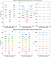 |
Fig. A.2 Same as Fig. A.1 for HST visit 12 (upper panels) and HST visit 22 (lower panels). |
| In the text | |
|
Fig. A.3 Reanalyzed, detrended literature u′-band light curves with the associated transit model described in Sect. 5.3. Bottom panels: associated residuals. |
| In the text | |
|
Fig. A.4 Reanalyzed, detrended literature B-band light curves with the associated transit model described in Sect. 5.3. Bottom panels: associated residuals. |
| In the text | |
|
Fig. A.5 Reanalyzed, detrended literature g′-band light curves with the associated transit model described in Sect. 5.3. Bottom panels: associated residuals. |
| In the text | |
|
Fig. A.6 Reanalyzed, detrended literature V -band light curves with the associated transit model described in Sect. 5.3. Bottom panels: associated residuals. |
| In the text | |
|
Fig. A.7 Reanalyzed, detrended literature r′-band light curves with the associated transit model described in Sect. 5.3. Bottom panels: associated residuals. |
| In the text | |
|
Fig. A.8 Reanalyzed, detrended literature R-band light curves with the associated transit model described in Sect. 5.3. Bottom panels: associated residuals. |
| In the text | |
|
Fig. A.9 Reanalyzed, detrended literature two i′-band (upper panels) and two z′-band (lower panels) light curves with the associated transit model described in Sect. 5.3. Bottom panels: associated residuals. |
| In the text | |
Current usage metrics show cumulative count of Article Views (full-text article views including HTML views, PDF and ePub downloads, according to the available data) and Abstracts Views on Vision4Press platform.
Data correspond to usage on the plateform after 2015. The current usage metrics is available 48-96 hours after online publication and is updated daily on week days.
Initial download of the metrics may take a while.