| Issue |
A&A
Volume 620, December 2018
|
|
|---|---|---|
| Article Number | A74 | |
| Number of page(s) | 13 | |
| Section | Catalogs and data | |
| DOI | https://doi.org/10.1051/0004-6361/201833677 | |
| Published online | 03 December 2018 | |
Deep LOFAR 150 MHz imaging of the Boötes field: Unveiling the faint low-frequency sky⋆
1
Leiden Observatory, Leiden University, PO Box 9513, 2300 RA, Leiden, The Netherlands
e-mail: edwinretana@gmail.com
2
INAF – Istituto di Radioastronomia, via P. Gobetti 101, 40129 Bologna, Italy
3
SUPA, Institute for Astronomy, Royal Observatory, Blackford Hill, Edinburgh, EH9 3HJ, UK
4
Hamburger Sternwarte, University of Hamburg, Gojenbergsweg 112, 21029 Hamburg, Germany
Received:
19
June
2018
Accepted:
5
July
2018
We have conducted a deep survey (with a central rms of 55 μJy) with the LOw Frequency ARray (LOFAR) at 120–168 MHz of the Boötes field, with an angular resolution of 3.98″ × 6.45″, and obtained a sample of 10 091 radio sources (5σ limit) over an area of 20 deg2. The astrometry and flux scale accuracy of our source catalog is investigated. The resolution bias, incompleteness and other systematic effects that could affect our source counts are discussed and accounted for. The derived 150 MHz source counts present a flattening below sub-mJy flux densities, that is in agreement with previous results from high- and low- frequency surveys. This flattening has been argued to be due to an increasing contribution of star-forming galaxies and faint active galactic nuclei. Additionally, we use our observations to evaluate the contribution of cosmic variance to the scatter in source counts measurements. The latter is achieved by dividing our Boötes mosaic into 10 non-overlapping circular sectors, each one with an approximate area of 2 deg2. The counts in each sector are computed in the same way as done for the entire mosaic. By comparing the induced scatter with that of counts obtained from depth observations scaled to 150 MHz, we find that the 1σ scatter due to cosmic variance is larger than the Poissonian errors of the source counts, and it may explain the dispersion from previously reported depth source counts at flux densities S < 1 mJy. This work demonstrates the feasibility of achieving deep radio imaging at low-frequencies with LOFAR.
Key words: surveys / catalogs / radio continuum: general / techniques: image processing
The source catalog and mosaic image are only available at the CDS via anonymous ftp to cdsarc.u-strasbg.fr (130.79.128.5) or via http://cdsarc.u-strasbg.fr/viz-bin/qcat?J/A+A/620/A74
© ESO 2018
1. Introduction
The most luminous radio sources are often associated with radio-loud active galactic nuclei (AGN) powered by accretion onto supermassive black holes (SMBHs), whose radio emission is generated by the conversion of potential energy into electromagnetic energy released as synchrotron radiation and manifesting itself as large-scale structures (radio jets and lobes). The less luminous radio-selected objects are mostly associated with accreting systems like radio-quiet AGNs or starburst galaxies. The radio-emission in star-forming systems has two components: a non-thermal synchrotronic component produced by cosmic rays originating from supernova shockwaves, and a thermal free-free component arising from the interstellar medium ionization by hot massive stars (Condon 1992). Star formation is also thought to be responsible at least for a fraction of radio emission in radio-quiet AGNs (Padovani et al. 2011; Condon et al. 2012).
In recent years, many studies have confirmed a flattening in the (Euclidean normalized) radio counts below a few mJy (Smolčić et al. 2008; Padovani et al. 2009) first detected more than three decades ago (Windhorst et al. 1985; Kellermann et al. 1986). This flatening is due to an increasing contribution of faint radio sources at sub-mJy flux densities. The precise fraction associated with different objects is still under debate, with studies showing a mixture of ellipticals, dwarf galaxies, high-z AGNs, and starburst galaxies (Padovani 2011; Smolčić et al. 2017b). The plethora of objects found suggests a complex interplay between star-formation (SF) and AGN activity in the universe.
Additional efforts are important to understand the physical processes that trigger the radio emission of the sub-mJy and microJy sources. Currently, this is partly hampered because the required sensitivity to detect fainter objects have been achieved in only a few small patches of the sky (Schinnerer et al. 2010; Condon et al. 2012; Miller et al. 2013; Vernstrom et al. 2016; Smolčić et al. 2017a).
The majority of deep surveys (Schinnerer et al. 2010; White et al. 2012; Miller et al. 2013; Vernstrom et al. 2016; Smolčić et al. 2017a) have been carried using radio telescopes operating at high-frequencies (> 1.0 GHz). This situation is rapidly changing as the number of low-frequency radio surveys (< 1.0 GHz) has increased in the last few years. Some survey examples include the VLA Low frequency Sky Survey (VLSS; Cohen et al. 2007), Murchison Widefield Array (MWA) Galactic and Extragalactic All-sky MWA survey (GLEAM; Wayth et al. 2015), and the LOFAR Two-metre Sky Survey (LoTSS; Shimwell et al. 2017). However, several challenges such as strong radio interference and varying effects like ionospheric phase errors across the instrument field of view (FOV) make producing high-resolution, low-frequency radio maps a difficult task (Noordam 2004). The necessity to overcome these challenges and to fully exploit the science offered by low-frequency telescopes has spurred an invigorated interest by radio-astronomers in improving the low-frequency calibration and imaging techniques (e.g. Cotton et al. 2004; Intema et al. 2009; Kazemi et al. 2011; Smirnov 2011; van Weeren et al. 2016; Tasse et al. 2018).
The LOFAR Surveys Key Science Project (SKSP) is embarking on a survey with three tiers of observations: the LoTSS survey at Tier-1 level covers the largest area at the lowest sensitivity (≳100 μ Jy) covering the whole 2π steradians of the northern sky. Deeper Tier-2 and Tier-3 programs aim to cover smaller fields with extensive multi-wavelength data up to a depth of tens and a few microJy, respectively (see Röttgering et al. 2011). Together these surveys will open the low-frequency electromagnetic spectrum for exploration, allowing unprecedented studies of the faint radio population across cosmic time and opening up new parameter space for searches for rare, unusual objects such as high-z quasars (Retana-Montenegro & Röttgering 2018) in a systematic way (see Fig. 1).
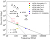 |
Fig. 1. Comparison between two radio sources with the same flux, but different spectral indices. The black triangles denote the 5σ flux density limits for previous all-sky shallow low- and high- frequency surveys (Hales et al. 1988; Becker et al. 1995; Condon et al. 1998; Rengelink et al. 1997; Cohen et al. 2007; Heald et al. 2015; Intema et al. 2017), while color bars indicate the 3 different tiers for LOFAR surveys using the LOFAR Low band antennas (LBA) and High band antennas (HBA), and the deepest high-frequency surveys currently published (Schinnerer et al. 2010; Miller et al. 2013; Smolčić et al. 2017a). Sources steeper than α = −2.1 will be detected at higher signifcance in the Tier-2/Tier-3 surveys than in deep high-frequency surveys, while sources flatter than α = −0.75 at detected at both low and high frequencies. |
One of the regions for the Tier-2 and Tier-3 radio-continuum surveys is the Boötes field. This 9.2 deg2 region is one of the NOAO Deep Wide Field Survey (NDWFS; Jannuzi & Dey 1999) fields, and has a large wealth of multi-wavelength data available including: X-rays (Chandra; Kenter et al. 2005), optical (Uspec, BW, R, I, z, Y bands; Jannuzi & Dey 1999; Cool 2007; Bian et al. 2013), infrared (J, H, K bands, Spitzer; Autry et al. 2003; Ashby et al. 2009; Jannuzi et al. 2010), and radio (60–1400 MHz; de Vries et al. 2002; Williams et al. 2013, 2016; van Weeren et al. 2014).
In this work, we present deep 150 MHz LOFAR observations of the Boötes field obtained using the facet calibration technique described by van Weeren et al. (2016). The data reduction and analysis for other deep fields using the kMS approach (Tasse 2014; Smirnov & Tasse 2015) and DDFACET imager (Tasse et al. 2018) will be presented in future papers (Mandal, in prep.; Sabater, in prep.; Tasse, in prep.). This paper is structured as follows. In Sects. 2 and 3, we describe the observations and data reduction, respectevely. We present our image and source catalog in Sect. 4. We also discuss for the flux density scale, astrometry accuracy, and completeness and reliability. The differential source counts are presented and discussed in Sect. 5. The contribution of cosmic variance to the scatter in source counts measurements is also discussed in Sect. 5. Finally, we summarise our conclusions in Sect. 6. We assume the convection Sν ∝ ν−α, where ν is the frequency, α is the spectral index, and Sν is the flux density as function of frequency.
2. Observations
The Boötes observations centered at 14h32m00s +34d30m00s (J2000 coordinates) were obtained with the LOFAR high band antenna (HBA). We combine 7 datasets observed from March 2013 (Cycle 0) to October 2015 (Cycle 4), which correspond aproximately to a total observing time of 55 hours. When the LOFAR stations operate in the “HBA DUAL INNER” configuration at 150 MHz, LOFAR has a half-power beam width (HPBW) of ∼5° with an angular resolution of ∼5″ (using only the central and remote stations located in The Netherlands). 3C196 is used as primary flux calibrator and was observed 10 min prior to the target observation. The nearby radio-loud quasar 3C295 was selected as secondary flux calibrator, and was observed for 10 min after the target. The observations from cycles 0 and 2 consist of 366 subbands covering the range 110–182 MHz. The subbands below 120 MHz and above 167 MHz generally present poor signal-to-noise (S/N). Therefore, in the following cycles, to obtain a more efficient use of the LOFAR bandwidth the frequency range was restricted to 120–167 MHz, resulting in only 243 subbands per observation. The total time on target varies depending on the cycle. The two observations from Cycle 0 are 5 h and 10 h long, whereas Boötes was observed for 8 h per observation in Cycles 2 and 4. The frequency and time resolution for the observations varies for each cycle. Table 1 presents the details for each one of the observations used in our analysis. Our observations include the dataset L240772 analyzed by Williams et al. (2016).
Summary of the LOFAR Boötes observations.
3. Data reduction
In this section, the data reduction steps of the LOFAR data processing are briefly explained. These steps are divided into three stages: the calibration into a non-directional and directional-dependent parts, and the combination of the final calibrated datasets. We refer the reader to the works of van Weeren et al. (2016) and Williams et al. (2016) for a more detailed explanation of the calibration procedure.
3.1. Direction independent calibration
First, we start by downloading the unaveraged data from the LOFAR Long Term Archive (LTA)1. We follow the basic sequence of steps for the direction-independent (DI) calibration: basic flagging and RFI removal employing AOflagger (Offringa et al. 2010, 2012); flagging of the contributing flux associated to bright off-axis sources referred as the A-team (Cyg A, Cas A, Vir A, and Tau A); obtaining XX and YY gain solution towards the primary flux calibrator using a 3C196 skymodel provided by Pandey (priv. comm.); determining the clock offsets between core and remote stations using the primary flux calibrator phases solutions as described by van Weeren et al. (2016); measuring the XX and YY phase offsets for the calibrator; transferring of amplitude, clock values and phase offsets to the target field; averaging each subband to a resolution of 4 s and 4 channels (no averaging is done for cycle 0 data); initial phase calibration of the amplitude corrected target field using a LOFAR skymodel of Boötes. The final products from the DI calibration are fiducial datasets consisting of 10 subbands equivalent to 2 MHz bands. Each observation is composed of 23 or 21 bands depending on the number of bands flagged due to RFI. We limit the frequency to the range 120–167 MHz to accomplish an uniform coverage in the frequency domain.
The DI calibrated bands are imaged at medium-resolution (∼40″ × 30″) using wsclean2 (Offringa et al. 2014). From these images, we construct a medium-resolution skymodel that is subtracted from the visibility data. Later, these data are imaged at low-resolution (∼110″ × 93″) to obtain a low-resolution skymodel. This two-stage approach allows to include extended emission that could have been missed in the medium-resolution image. Both medium- and low-resolution skymodels are combined to create the band skymodel. Finally, the band skymodel is used to subtract the sources from the UV data to obtain DI residual visibilities. This subtraction is temporarily, as these sources will be added later in the directional self-calibration process. This stage of the data processing is carried out using the prefactor3 tool.
3.2. Direction dependent calibration
Direction-dependent (DD) effects such as the spatial and temporal variability of the LOFAR station beam response, and the ionospheric distortions must be considered to obtain high-fidelity low-frequency radio images. It is well known that these effects are responsible for artifacts and higher noise levels in low-frequency images (e.g. Yatawatta et al. 2013). A simple approach to correct these DD effects was originally proposed by Schwab (1984). If the variation of the DD effects across the field of view (FOV) is smooth, we can divide the FOV into a discrete number of regions or “facets”. Within each facet, there needs to be a bright source or group of closely spaced bright sources, which is designated as the facet calibrator. A self-calibration process can be performed on each facet calibrator. This yields a set of DD calibration solutions that are used to calibrate the whole facet. With the DD solutions applied an image of the facet is made and a model for the sources is created. Subsequently, this model is subtracted from the visibility data, and the next brightest facet is dealt with (Noordam 2004). By executing these steps in an iterative way, it is possible to correct the DD effects for all the facets in the FOV. Here, we adopt the DD calibration technique described by van Weeren et al. (2016) to process LOFAR HBA datasets. This procedure is now implemented in the factor4 pipeline.
In our data processing, we use the same facet calibrator distribution as Williams et al. (2016) with new boundary geometry (see Fig. 2). The range of the flux density for our facet calibrators is between 0.3 mJy and 2 Jy. To start the DD process, the corresponding facet calibrator, which was subtracted at the end of the DI calibration is added back to the UV data, and all the bands are phase-rotated in the direction of the calibrator. The self-calibration process comprises several cycles. In the first and second cycles, we solve for the phase-offsets and the total ionospheric electron content (TEC) terms (which introduces a frequency-dependent ionospheric distortion on the phases offsets) only on timescales of ∼10 s. For the third and fourth cycles, we initially solve only for phase+TEC. Finally, we obtain phase+amplitude solutions on large timescales (> 5 min for bright calibrators) to mainly capture the relative slow variations in the beam. The last self-calibration cycle can be iterated various times until convergence is achieved. This last iteration step helps to decrease the number of artifacts around bright facet calibrators.
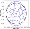 |
Fig. 2. The spatial distribution of the facets in the Boötes field (blue solid lines). The large circle (solid black line) indicates the radial cutoff of 2.5° used to apply the primary beam correction. |
The imaging of the facet starts when the sources not selected as facet calibrators are added back to the UV data and the DD solutions are applied. The facet is imaged in two stages with wsclean (Offringa et al. 2014). First, it is imaged at high resolution (∼5″) to include all the compact sources in a high-resolution facet skymodel. Secondly, the brightest sources from the high-resolution skymodel are subtracted, and the facet is imaged at low-resolution ( ∼ 25″) to obtain a skymodel that includes diffuse emission that can be missed during the high-resolution imaging step. Both high and low resolution models are combined into a new updated skymodel for the facet that is subtracted from the full data. This process does not only improve the DI residual visibilities by reducing the effective noise in the UV data as the source subtraction is performed now using the DD solutions, but also suppresses the effect of the presence of bright calibrators on the subsequent subtraction of fainter facets. The facets are processed in a serial sequence, which is ordered in descending order according to the facet calibrator flux density.
3.3. Combined facet imaging
The procedure to combine different observations is summarized in the following steps:
-
Shifting to a common phase center. For each facet, the astrometry ultimately depends on the precision of the calibration model of the facet calibrator. This implies that the astrometry can be shifted between different regions due to the differences in precision between the models of facet calibrators. This also explains the reason why the astrometry for the same facet is usually slightly shifted, compared to that of other observations. To account for the astrometry offsets between different observations, we phase-shift all the data corresponding to the same facet to a common phase center.
-
Normalizing imaging weights. The data from cycle 0 (4ch,5s) has been further time averaged in comparison with the data from cycles 2 and 4 (4ch,4s). Thus, the imaging weights of cycle 0 data are multiplied by a factor of 1.25 to account for the extra time averaging.
-
Facet imaging. The phase-shifted datasets from all the observations corresponding to a facet are imaged together with wsclean. We use a pixel size of 1.5″, and a robust parameter of −0.7 to obtain a more uniform weighting between short and remote baselines.
-
Mosaicing and primary-beam correction. The resulting facets from the imaging step are mosaiced using factor. To apply the primary beam correction, we use a beam model created by wsclean. The correction is carried out by dividing the facet images by the regridded wsclean beam model. We impose a radial cutoff where the sensitivity of the phased array beam is 50 percent of that at the pointing center (i.e. a radius of ∼2.5 °).
4. Images and sources catalog
4.1. Final mosaic
The final mosaic has an angular resolution of 3.98″ × 6.45″ with PA = 103° and a central rms of ∼55 μJy beam−1 . The entire mosaic and the central region of the Boötes field are shown in Figs. 3 and 4, respectively.
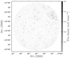 |
Fig. 3. LOFAR 150 MHz mosaic of the Boötes field after beam correction. The size of the mosaic is approximately 20 deg2. The synthesised beam size is 3.98″ × 6.45″. The color scale varies from −0.5σc to 10σc, where σc = 55 μJy beam−1 is the rms noise in the central region. |
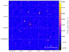 |
Fig. 4. Map showing the central 400′×400′ region of the mosaic center after primary beam correction. The synthesized beam size is 3.98″ × 6.45″. The color scale varies from −6σl to 16σl, where σ1 = 55 μJy beam−1 is the local rms noise. |
4.2. Noise analysis and source extraction
We evaluate the spatial variation of the sensitivity of our mosaic using a noise map created by PyBDSF5(the Python Blob Dectection and Source Finder, formerly PyBDSM; Mohan & Rafferty 2015). The noise map of the Boötes mosaic is shown in Fig. 5. The noise threshold varies from ∼55 μJy beam−1 in the central region to ∼180 μJy beam−1 at the mosaic edges. Around bright sources (> 500 mJy beam−1), the image noise can increase up to 5 times that of an unaffected region. This is caused by residual phase errors still present after DD calibration. The total area in which a source with a given flux can be detected, or visibility area, of our mosaic is displayed in Fig. 6. As expected, the visibility area increases rapidly between ∼55 μJy beam−1 to ∼250 μJy beam−1, with approximately 90 percent of the mosaic area having a rms noise less than 160 μJy beam−1. Two facets located near the mosaic edge have relatively higher noise levels in comparison with adjacent facets. In these regions, the DD calibration fails as their facet calibrators have low flux densities (S150 MHz < 1 mJy) resulting in amplitude and/or phase solutions with low S/Ns. The application of these poor solutions to the data gives as result high-noise facets (σ > 120 − 150 μJy beam−1) in the mosaic.
The software package PyBDSF was used to build an initial source catalog within the chosen radial cutoff. The initial source catalog consists of 10 091 sources detected above a 5σ peak flux density threshold. Of these 1978 are identified by PyBDSF with the source structure code “M” (i.e. sources with multiple components or complex structure), and the rest are classified as “S” (i.e. fitted by a single gaussian component). We inspected our mosaic and found 170 multi-component sources that are misclassified into different single sources by PyBDSF as their emission does not overlap. This includes the 54 extended sources identified by Williams et al. (2016). The components for such sources are merged together by 1) assigning the total flux from all the components as the total flux of the new merged source, 2) assigning the peak flux of the brightest component as the peak flux of the new merged source, and 3) computing the flux-weighted mean position of the components and assigning it as the position of the source. We list these merged sources as “Flag_merged” in the final source catalog.
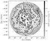 |
Fig. 5. Noise map of the LOFAR 150 MHz mosaic of the Boötes field after primary beam correction. The color scale varies from 0.5σc to 9σc, where σc = 55 μJy beam−1 is the rms noise in the central region. Contours are plotted at 70 μJy beam−1 and 110 μJy beam−1. |
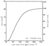 |
Fig. 6. Visibility area of the LOFAR image of the Boötes field. The full area covered is 20 deg2. |
We visually inspected the surroundings of bright objects to identify fake detections. A total of 119 objects are identified as artifacts and flagged “Flag_artifact” in our final catalog. These objects are excluded from our source counts calculations (see Sect. 6).
4.3. Astrometry
To check the positional accuracy, the LOFAR data is cross-correlated against the FIRST survey (Becker et al. 1995). We crossmatched the two catalogs using a matching radius of 2″. In order to minimize the possibility of mismatching, we consider only LOFAR sources with the following criteria: i) a S/N > 10 in both LOFAR and FIRST maps (i.e. high S/N sources), and ii) an angular size less than 50″ to select only compact sources with reliable positions. We find that the mean offsets in right ascension and declination for the cross-matched 989 LOFAR sources are ⟨α⟩ = 0.012 ± 1 × 10⁻⁴ arcsec and ⟨δ⟩ = 0.27 ± 1 × 10⁻⁴ arcsec, respectively. The standard deviations of the right ascension and declination are σRA = 0.57 arcsec and σDec = 0.64 arcsec, respectively. The examination of the offsets in the right ascension and declination directions shows that these have an asymmetrical distribution that differs between facets (see Fig. 7, left panels). We correct the positional offsets in both directions using the FIRST catalog for each facet independently. This is done by fitting a 2D plane to the offsets between the LOFAR and FIRST positions. The plane is A0(α−α0) + B0(δ−δ0) + C0 = 0, where α and δ are the right ascension and declination of the LOFAR-FIRST sources, respectively, α0 and δ0 are the central right ascension and declination of the corresponding facet, and the constants A0, B0, and C0 have units of arcseconds. This fitting provides the astrometry correction that is applied to all sources withing the corresponding facet (see Fig. 7, right panels). We find a total of selected 1048 LOFAR/FIRST sources after the corrections are applied. The mean offsets for the corrected positions are ⟨α⟩ = 0.009 ± 1 × 10⁻⁴ arcsec and ⟨δ⟩ = 0.005 ± 3 × 10⁻⁴ arcsec, respectively. The standard deviations are σRA = 0.42 arcsec and σDec = 0.40 arcsec, respectively. Figure 8 shows the corrected positional offsets. As these offsets are typically smaller than the pixel scale in our mosaic, we do not apply any further corrections for positional offsets in our catalog.
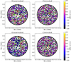 |
Fig. 7. Spatial distribution of positional offsets uncorrected (left panels) and corrected (right panels) between high S/N and compact LOFAR sources and their FIRST counterparts in the right ascention (top panels) and declination (bottom panels) directions. The colorbar denotes the offsets for each object. We find 989 LOFAR/FIRST sources (left panels) using the uncorrected positions; when the astrometry corrections are applied a total of 1048 LOFAR/FIRST sources are found (right panels). The black circle indicates the radial cutoff used to apply the primary beam correction, while the green lines show the facet distribution in our Boötes mosaic. |
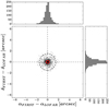 |
Fig. 8. Corrected positional offsets between high S/N and compact LOFAR sources and their FIRST counterparts (see text for more details). The dashed lines denotes a circle with radius r = 1.5″, which is the image pixel scale. The ellipse (red solid line) centered on the right ascension and declination mean offsets indicates the standard deviation for both directions. |
4.4. Bandwidth and time smearing
Two systematic effects that must be accounted for are bandwidth and time smearing. This combined smearing effect reduces the peak flux of a source, and simultaneously the source size is distorted or blurred in such way that the total flux is conserved, but the peak flux is reduced. The smearing effect depends on resolution, channel width, integration time, and increases with the source distance from the phase center. Williams et al. (2016) averaged their data to a resolution of 2 channels and 8 s, which yields a peak flux decrease of 21 percent at 2.5° from the pointing center according to the equations given by Bridle & Schwab (1999). In this work, the reduction in peak flux is less severe as our averaging factor is two times smaller in frequency and time. This results in a reduction of roughly 14 percent at the same distance. This holds for all the datasets that were not observed in cycle 0. For cycle 0 observations, the resolution available is 4 channel and 5 s. In this case, the peak flux underestimation is approximately 30 percent at 2.5° from the pointing center. Following Bridle & Schwab (1999), we apply a weighted smearing correction that takes into account the frequency resolution and integration time of the data sets. The factor for Cycle 0 observations is 15/55 = 0.27 (i.e. the ratio between the observing time obtained in Cycle 0 and the total observing time), and for the other cycles the factor is 40/55 (i.e. its reciprocal 0.73). The smearing correction factor (≥1.0) depends on the distance of the source from the pointing center.
4.5. Flux density scale accuracy
To verify the flux density scale for our Boötes catalog and check its consistency with the Scaife & Heald (2012) flux scale, we compare our fluxes with the GMRT 150 MHz Boötes catalog by Williams et al. (2013). These authors obtained a mosaic with rms levels of 2 − 5 mJy and an angular resolution of 25 arcsec. First, a representative sample of sources is chosen using the following criteria: i) a S/N > 15 in both LOFAR and GMRT maps (i.e. high S/N sources), ii) an angular size less than 50″, and iii) no neighbors within a distance equal to the GMRT beam size or 25″ (i.e. isolated sources). Secondly, we use a scaling factor of 1.078 to put the GMRT fluxes on the Scaife & Heald (2012) scale, according to the 3C196 calibration model (Williams et al. 2016). The crossmatching yields a total of 1250 LOFAR/GMRT sources. We find a mean flux ratio of fR = 0.88 with a standard deviation of σfR = 0.15, which indicates a systematic offset in our flux scale in comparison with the GMRT fluxes. Thus, we apply a correction factor of 12 percent to our LOFAR fluxes. After correcting the fluxes, we find a mean flux ratio of fR = 1.00 with a standard deviation of σfR = 0.12 (see Fig. 9). Considering uncertainties on the flux scale such as: the accuracy of the fluxes on LOFAR images obtained using skymodels based on the Scaife & Heald (2012) is approximately of 10 percent (e.g. Mahony et al. 2016; Shimwell et al. 2017), the errors of the GMRT flux scale (Williams et al. 2016), and the differences in elevation between the calibrator and target, we conclude that a 15 percent uncertainty in our flux scale is appropriate. These global errors are added in quadrature to the flux uncertainties reported by PyBDSF in our final catalog.
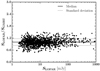 |
Fig. 9. Total flux ratio for LOFAR sources and their GMRT counterparts. Only unresolved and isolated LOFAR sources with S/N > 15 are considered (see text for more details). The dashed lines correspond to a standard deviation of σfR = 0.12, and the median ratio of 1.00 is indicated by a solid black line. |
4.6. Resolved sources
We estimate the maximum extension of a radio source using the total flux ST to peak flux SP ratio:

where θmin and θmaj are the source FWHM axes, bmin and bmaj are the synthesized beam FWHM axes. The correlation between the peak and total flux errors produces a flux ratio distribution with skewer values at low S/N, while it has a tail due to extented sources that extends to high ratios (Prandoni et al. 2000). If ST/SP < 1 sources are affected by errors introduced by the noise in our mosaic, we can derive a criterion for extension assuming that these errors affect ST/SP > 1 sources as well. The lower envelope (the curve that contains 90 percent of all sources with SP < ST) is fitted in the SP/σ axis (where σ is the local rms noise). This curved is mirrored above the SP = ST axis, and is described by the equation:
![$$ \begin{aligned} S_{\rm T}/S_{\rm P}=1.09+\left[\frac{2.7}{(S_{\rm P}/\sigma )}\right]\cdot \end{aligned} $$](/articles/aa/full_html/2018/12/aa33677-18/aa33677-18-eq2.gif)
Using the upper envelope, we find that 4292 of 10 091 (i.e. 42 percent) of the sources in our catalog can be considered extended (see Fig. 10, right panel). These sources are listed as resolved in the final catalog (Sect. 4.8). However, still some objects classified by PyBDSF as made of multiple components are not identified by this criterion as resolved. Similarly, point sources could be located above the envelope by chance.
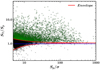 |
Fig. 10. Ratio of the total flux density ST to peak flux density SP as a function of S/N (SP/σ) for all sources in our catalog. The red lines indicate the lower and upper envelopes. The blue line denotes the ST = SP axis. Sources (green circles) that lie above the upper envelope are considered to be resolved. |
4.7. Completeness and reliability
The incompleteness in radio surveys is mainly an issue at low S/Ns, where a significant fraction of the sources can be missed. This is consequence of the image noise on the source detection. For instance, at the detection threshold sources that are located on random noise peaks are more easily detected than those located on noise dips (Prandoni et al. 2000).
The fraction of sources detected at 5σ in the mosaic is estimated through Monte-Carlo (MC) simulations. First, we insert artificial point sources into the residual map created by PyBDSF (see Sect. 4.2). We generate 30 random catalogs with an artificial source density of at least three times the real catalog. These artificial sources are placed at random locations in the residual map. The fluxes are drawn from a power-law distribution inferred from the real sources, with a range between 0.5σ and 30σ, where σ = 55 μJy beam−1. The source extraction is performed with the same parameters as for the real mosaic. To obtain a realistic distribution of sources, 40 percent of the objects in our simulated catalogs are taken to be extended. In the MC simulations, the extended sources are modeled as objects with a gaussian morphology. Their major axis sizes are drawn randomly from values between one and two times the synthesized beam size, the minor axis sizes are chosen to have a fraction between 0.5 and 1.0 of the corresponding major axis size, and the position angles are randomly selected between 0° and 180°. We determine the completeness at a specific flux ST by evaluating the integral distribution of the detected source fraction with total flux > ST. The detected fraction and completeness of our catalog are shown in Fig. 11. Our results indicate that at ST > 1 mJy, our catalog is 95 percent complete, whereas at ST ≲ 0.5 mJy the completeness drops to about 80 percent.
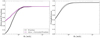 |
Fig. 11. Left panel: fraction of sources detected in our simulations (solid black line) and detected fraction corrected for the visibility area that is used in the source counts calculation (solid purple line). Right panel: completeness function of our Boötes catalog as a function of flux density. Our catalog is 95 percent complete at S150 MHz > 1 mJy, while the completeness drops to about 80 percent at ST ≲ 0.5 mJy. The dashed lines in both plots represent 1σ errors estimated using Poisson statistics. |
In our facets, the presence of residual amplitude and phase errors causes the background noise to deviate from a purely Gaussian distribution. These noise deviations could be potentially detected by the source-finding algorithm as real sources. Assuming that the noise deviations can be equally likely negative or positive and real detections are due to positive peaks only, we run PyBDSF on the inverted mosaic as done in Sect. 4.2 to estimate the false detection rate (FDR) in our survey. This negative mosaic is created by multiplying all the pixels in the mosaic image by −1. During our tests in the negative mosaic, we discovered that PyBDSF identifies a large number of artifacts around bright sources as “real” sources. This could potentially bias our FDR estimations. Therefore, we mask the regions around bright sources (ST > 200 mJy) with circle of radius 25″ to make certain that our FDR estimations are not dominated by artifacts. Excluding bright sources does not affect our FDR estimations, as FDR is generally relevant for fainter sources, whese noise deviations could be detected as real objects. The FDR is determined from the ratio between the number of false detections and real detections at a specific flux density bin. The reliability, R = 1−FDR at a given flux density S, is estimated by integrating the FDR over all fluxes > S. The FDR and reliability are plotted as a function of total flux density in Fig. 12.
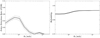 |
Fig. 12. Left panel: false detection rate (FDR) as a function of flux density. For ST < 1 mJy, the FDR is less than 5 percent, while there are not false detections for ST > 5 mJy. Right panel: reliability function of our Boötes catalog as a function of flux density. The dashed lines in both plots represent 1σ errors estimated using Poisson statistics. |
A sample of ten rows from the source catalog.
4.8. Source catalog
The final catalog and mosaic image containing 10 091 sources detected above a 5σ flux density threshold are made available at the CDS. The astrometry, total and peak flux densities in the catalog are corrected as described in Sects. 4.3–4.5 respectively. The reported flux densities are on the Scaife & Heald (2012) flux density scale and their errors have the global uncertainties added in quadrature as described in Sect. 4.5. We list a sample from 13 rows of the published catalog in Table 2, where the columns are:
-
(1)
Source ID,
-
(2,4)
source position (RA, Dec),
-
(3,5)
errors in source position,
-
(6,7)
total flux density and error,
-
(8,9)
peak flux density and error,
-
(10)
combined bandwidth and time smearing correction factor for the peak flux density,
-
(11)
local rms noise,
-
(12)
source type (point source or extended),
-
(13)
PyBDSF source structure code (S/M).
-
(13)
Flag edge, when equals to 1 indicates an object that is located close to or in a facet edge, which could result in some flux loss.
-
(14)
Flag artifact, this flag indicate if an object is a calibration artifact: a value of “1” signifies a source that is probably an artifact, and “2” signifies that is surely an artifact.
-
(15)
Flag merged, when equal to 1 indicates a large diffuse source whose separate components are merged into a single one according to a visual inspection.
5. Source counts
5.1. Size distribution and resolution bias
Following Prandoni et al. (2001), we use estimate an upper limit Θlim for the angular size that a source of given flux can have before its peak flux falls below our detection threshold (5σ). This upper limit is defined as a function of the total flux density:

where Θmax is obtained utilizing Eq. (1) and Θmin, the minimum angular size that is reliably resolved, can be derived combining Eqs. (1) and (2). The constraint provided by Θmin takes into account the finite size of the synthesized beam and ensures that Θlim does not become unphysical (Θmax → 0 at low S/Ns). Sources with sizes > Θmax will remain undetected and the resulting catalog will be incomplete, whereas for sources with sizes < Θmin the deconvolution is not reliable. This systematic effect is called resolution bias. The range of possible values for the Θmax and Θmin according to our rms levels are indicated by the green and yellow, respectively, shaded lines in Fig. 13. To define the rms levels, we consider minimum and maximum noise values in our map. As shown in Fig. 6, 90 percent of the total area has approximately σ ≲ 140 μJy. This value can thus be considered as representative of the maximum noise value. For the minimum noise value, we take the central rms noise in our map that is about σ ∼ 55 μJy. The (deconvolved) size distribution of our sources is shown in Fig. 13. As expected our sources tend to be smaller than the maximum allowed sizes.
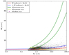 |
Fig. 13. Angular size (deconvolved geometric mean) for LOFAR sources as function of their total flux density. The range of possible values for the maximum and minimum detectable angular sizes corresponding to the rms range in our mosaic (55 − 140 μJy) are indicated by the green and yellow lines, respectively. All unresolved sources are located in the plane Θ = 0, and the median source sizes for our sample are shown by purple points. The red line indicates the median of the Windhorst et al. (1990) functions, the blue line represents the same function increased by a normalization factor of 2. |
A good knowledge of the angular size distribution of our LOFAR sources is critical for a correct determination of the resolution bias in our survey. Particularly, at low-frequencies the sources can be more extended, and the size distribution can be different from that estimated in GHz surveys (Williams et al. 2016; Mahony et al. 2016). In Fig. 13, we compare the median of the angular size for our sample (purple points) with the average of the two median size relations proposed by Windhorst et al. (1990, 1993) for 1.4 GHz surveys:
after scaling them to 150 MHz using a spectral index of α = − 0.7 (Smolčić et al. 2017a; red solid lines). It is clear that our sources have larger median deconvolved angular sizes than those predicted by the Windhorst relations. A similar trend was found by Mahony et al. (2016) and Williams et al. (2016) in their analysis of LOFAR observations. These authors proposed to modify the Windhorst relations by increasing the normalization by factor of 2 (blue solid line) to obtain a better fit to the median angular sizes for their sources. A close examination to the median source sizes in our sample indicates that this modification indeed provides a good fit to our data. Therefore, we employ this relation to account for the resolution effects in our catalog.
To correct the source counts for the incompleteness due to the resolution bias we need to determine the true integral angular size distribution of radio sources as a function of the total flux density. Windhorst et al. (1990) reported a exponential form for the true angular size distribution:
![$$ \begin{aligned} h\left(\Theta _{\mathrm{lim}}\right)=\exp \left[\left(b\left(\frac{\Theta _{\mathrm{lim}}}{\Theta _{\mathrm{med}}}\right)^{a}\right)\right], \end{aligned} $$](/articles/aa/full_html/2018/12/aa33677-18/aa33677-18-eq5.gif)
with a = −ln(2) and b = 0.62. To determine the unbiased integral size distribution from our sample, we need to select sources in a total flux density range that is not affected by the resolution bias. For this purpose, we choose the flux density range 10 mJy < ST < 25 mJy. The reason for choosing this flux density range is two fold. First, the number of reliably deconvolved sources in this range is 93 percent, and second to determine the integral size distribution with a large statistical sample that is close as possible to our 5σ detection threshold. In Fig. 14 (left panel), we compare the integral size distribution (solid black line) for sources in our catalog with flux densities in the range 10 mJy < S150 MHz < 25 mJy with the 1.4 GHz relations proposed by Windhorst scaled to 150 MHz using a spectral index of α = −0.7. We find that the scaled Windhorst relations are a good represention of the integral size distribution for Θ ≲ 5″ sources, which correspond to a fraction of 80 percent in our Boötes catalog.
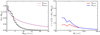 |
Fig. 14. Left panel: integral size distribution (black lines) for sources in our catalog with 10 mJy < S150 MHz < 25 mJy. The red and blue lines represent the Windhorst et al. (1990) and Windhorst et al. (1993) relations scaled to 150 MHz and increased by a normalization factor of 2 for the corresponding median angular sizes. Right panel: resolution bias c = 1/[1−h(Θlim)] as a function of the total flux density. The color legends are the same as in the left panel. |
The resolution bias correction is defined as c = 1/[1−h(Θlim)] (Prandoni et al. 2001). Figure 14 (right panel) shows the resolution bias correction as a function of the total flux density for the scaled Windhorst relations and the integral size distribution determined for our sample. We use the average of the Windhorst relations to apply the resolution bias correction to our catalog. Additionally, a 10 percent uncertainty is added in quadrature to the errors in the source counts following Windhorst et al. (1990).
5.2. Visibility area
The varying noise present in our mosaic implies that objects with different flux densities are not distributed uniformly in the region surveyed. Thus, the contribution of each object to the source counts is weighted by the reciprocal of its visibility area (i.e. the fraction of the total area in which the source can be detected), as derived in Sect. 4.2. This correction allows us to account for different visibility areas within the same flux density bin.
5.3. Completeness and reliability
As can be seen in Fig. 4.7, the fraction of detected sources decreases towards fainter flux densities. Thus, a correction factor that accounts for the missed objects is required when calculating the source counts. For this purpose, we employ the detected fraction corrected for the visibility area (see Fig. 11) to account for the incompleteness in our source counts. Furthermore, we apply a factor to account for the reliability using the FDR derived in Sect. 4.7.
5.4. Multiple-component sources
In Sect. 4.2, we carried out a visual inspection to identify resolved sources that have been misclassified into different single components by our source extraction software. However, for sources that are resolved out and split out into multiple-components and do not show signs of physical connection, establishing that their components are part of a same source is not trivial. Consequently, these components are still listed as separate sources in our catalog. This must be taken into account when computing the source counts to ensure these multi-component sources are only counted once. For this purpose, we employ the algorithm by Magliocchetti et al. (1998), to identity the missed double sources in our catalog. First, the separation between a component and its nearest neighbor, and the total flux density of the two components are compared. The components are considered as part of a double source if their flux ratio f is in the range 0.25 ≤ f ≤ 4, and satisfies the separation criterion scaled to 150 MHz using a spectral index of α = −0.7:
where Θ0 is in arcseconds and ST is the summed flux of the two components, otherwise the components are considered independent single sources . We identify 633 sources (i.e. 6 percent of the catalog) as doubles following the Magliocchetti et al. (1998) criterion.
5.5. Differential source counts
The normalized 150Hz differential radio-source counts derived from our LOFAR Boötes observations between our 5σ flux density threshold of 275 μJy and 3 Jy are shown in Fig. 16. Vertical error bars indicate the uncertainties obtained by propagating the errors on the correction factors to the  Poissonian errors (Gehrels 1986) from the raw counts. Horizontal error bars denote the flux bins width.
For comparison purposes, previous 150 MHz source counts by Intema et al. (2017) and Franzen et al. (2016), as well as the Boötes counts obtained by Williams et al. (2016) are shown in Fig. 16. Additionally, we show previous results from deep fields at 1.4 GHz (Padovani et al. 2015), 3 GHz (Smolčić et al. 2017a) and the compilation by de Zotti et al. (2010) scaled to 150 MHz using a spectral index of α = −0.7 (Smolčić et al. 2017a).
Our source counts are in fairly good agreement with previous low- and high- frequency surveys. At S150 MHz > 1 mJy, there is a very good consistency for the source counts derived from the various surveys. The situation is different for the fainter flux bins (S150MHz < 1 mJy), where there is a large dispersion between the results from the literature. In the range S150MHz ≤ 1.0 mJy, our source counts are consistent with those derived by Williams et al. (2016), and also they closely follow the counts reported by Smolčić et al. (2017a). In the flux density bins S150 MHz ≤ 0.4 mJy, the drop in the source counts may be the result of residual incompleteness. Our data confirms the change in the slope at sub-mJy flux densities previously reported in the literature by high- (Katgert et al. 1988; Hopkins et al. 1998; Padovani et al. 2015) and low- (Williams et al. 2016; Mahony et al. 2016) frequency surveys. This change can be associated to the increasing contribution of SF galaxies and radio-quiet AGNs at the faintest flux density bins (Smolčić et al. 2008, 2017b; Padovani et al. 2009, 2011).
5.6. Cosmic variance
The differences between source counts at flux densities < 1.0 mJy for multiple independent fields are generally larger than predicted from their Poissonian fluctuations (Condon 2007). These differences may result from either systematics uncertainties such as the calibration accuracy, primary beam correction, and bandwidth smearing, or different resolution bias corrections adopted in the literature, or cosmic variance introduced by the large scale structure. The combination of large area coverage and high sensitivity of our Boötes observations offers an excellent opportunity to investigate the effect of cosmic variance in the source counts from different extragalactic fields. For this purpose, we divide the 20 deg2 Boötes mosaic into 10 non-overlapping circular sectors, each one with an approximate area of 2 deg2 and on average containing more than 900 sources. Figure 15 shows the spatial distribution of the circular sectors in the Boötes mosaic.
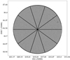 |
Fig. 15. Spatial distribution of the circular sectors in the Boötes mosaic used to test the effect of cosmic variance in our source counts. Each circular sector has an approximate area of 2 deg2. |
The purple shaded region in Fig. 16 shows the 1σ scatter due to cosmic variance in our source counts. The counts in each circular sector are computed in the same way as done for the entire mosaic. The comparison of the shaded region with the counts derived from deep observations scaled to 150 MHz suggests that the 1σ scatter due to cosmic variance is larger than the Poissonian errors of the source counts, and it may explain the dispersion from previously reported depth source counts at flux densities S < 1 mJy. This confirms the results of Heywood et al. (2013) who reached a similar conclusion by comparing the scatter of observed source counts with that of matched samples from the S3-SEX simulation by Wilman et al. (2008).
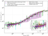 |
Fig. 16. Normalized 150Hz differential radio-source counts derived from our LOFAR Boötes observations between 275 μJy and 2 Jy (purple points). Vertical error bars are calculated assuming Poissonian statistics and horizontal error bars denote the flux bins width. Open black circles show the counts uncorrected for completeness and reliability. The purple shaded area displays the 1σ range of source counts derived from 10 non-overlapping circular sectors. For comparison, we overplot the source counts from recent deep and wide low-frequency surveys (Franzen et al. 2016; Intema et al. 2017), as well the source counts derived by Williams et al. (2016) in the Boötes field. In addition, the results of previous deep surveys carried out at 1.4 GHz (de Zotti et al. 2010; Padovani et al. 2015); and 3 GHz (Smolčić et al. 2017a) are scaled to 150 MHz using a spectral index of α = −0.7 (Smolčić et al. 2017a). The inset shows the source counts in the range 0.080 mJy ≤ S150 MHz ≤ 4 mJy. |
6. Conclusions
We have presented deep LOFAR observations at 150 MHz. These observations cover the entire Boötes field down to an rms noise level of ∼55 μJy beam−1 in the inner region, with a synthesized beam of 3.98″ × 6.45″. Our radio catalog contains 10 091 entries above the 5σ detection over an area of 20 deg2. We investigated the astrometry, flux scale accuracy and other systematics in our source catalog. Our radio source counts are in agreement with those derived from deep high-frequency surveys and recent low-frequency observations. Additionally, we confirm the sharp change in the counts slope at sub-mJy flux densities. The combination of large area coverage and high sensitivity of our Boötes observations suggests that the 1σ scatter due to cosmic variance is larger than the Poissonian errors of the source counts, and it may explain the dispersion from previously reported depth source counts at flux densities S < 1 mJy.
Our LOFAR observations combined with the Boötes ancillary data will allow us to perform a photometric identification of most of the newly detected radio sources in the catalog, including rare objects such as high-z quasars (Retana-Montenegro & Röttgering 2018). Future spectroscopic observations will provide an unique opportunity to study the nature of these faint low-frequency radio sources.
Acknowledgments
ERM acknowledges financial support from NWO Top project No. 614.001.006. HJAR and RJvW acknowledge support from the ERC Advanced Investigator program NewClusters 321271. PNB is grateful for support from the UK STFC via grant ST/M001229/1. LOFAR, the Low Frequency Array designed and constructed by ASTRON, has facilities in several countries, that are owned by various parties (each with their own funding sources), and that are collectively operated by the International LOFAR Telescope (ILT) foundation under a joint scientific policy. The Open University is incorporated by Royal Charter (RC 000391), an exempt charity in England & Wales and a charity registered in Scotland (SC 038302). The Open University is authorized and regulated by the Financial Conduct Authority.
References
- Ashby, M. L. N., Stern, D., Brodwin, M., et al. 2009, ApJ, 701, 428 [NASA ADS] [CrossRef] [Google Scholar]
- Autry, R. G., Probst, R. G., Starr, B. M., et al. 2003, Proc. SPIE, 4841, 525 [Google Scholar]
- Becker, R. H., White, R. L., & Helfand, D. J. 1995, ApJ, 450, 559 [NASA ADS] [CrossRef] [Google Scholar]
- Bian, F., Fan, X., Jiang, L., et al. 2013, ApJ, 774, 28 [NASA ADS] [CrossRef] [Google Scholar]
- Bridle, A. H., & Schwab, F. R. 2003, ASP Conf. Ser., 180, 371 [Google Scholar]
- Cohen, A. S., Lane, W. M., Cotton, W. D., et al. 2007, AJ, 134, 1245 [NASA ADS] [CrossRef] [Google Scholar]
- Condon, J. J. 1992, ARA&A, 30, 575 [NASA ADS] [CrossRef] [MathSciNet] [Google Scholar]
- Condon, J. J. 2007, ASP Conf. Ser., 380, 189 [NASA ADS] [Google Scholar]
- Condon, J. J., Cotton, W. D., Greisen, E. W., et al. 1998, AJ, 115, 1693 [NASA ADS] [CrossRef] [Google Scholar]
- Condon, J. J., Cotton, W. D., Fomalont, E. B., et al. 2012, ApJ, 758, 23 [NASA ADS] [CrossRef] [Google Scholar]
- Cool, R. J. 2007, ApJS, 169, 21 [NASA ADS] [CrossRef] [Google Scholar]
- Cotton, W. D., Condon, J. J., Perley, R. A., et al. 2004, Proc. SPIE, 5489, 180 [Google Scholar]
- de Vries, W. H., Morganti, R., Röttgering, H. J. A., et al. 2002, AJ, 123, 1784 [NASA ADS] [CrossRef] [Google Scholar]
- de Zotti, G., Massardi, M., Negrello, M., & Wall, J. 2010, A&ARv, 18, 1 [NASA ADS] [CrossRef] [Google Scholar]
- Franzen, T. M. O., Jackson, C. A., Offringa, A. R., et al. 2016, MNRAS, 459, 3314 [NASA ADS] [CrossRef] [Google Scholar]
- Gehrels, N. 1986, ApJ, 303, 336 [NASA ADS] [CrossRef] [Google Scholar]
- Hales, S. E. G., Baldwin, J. E., & Warner, P. J. 1988, MNRAS, 234, 919 [Google Scholar]
- Heald, G. H., Pizzo, R. F., Orrú, E., et al. 2015, A&A, 582, A123 [NASA ADS] [CrossRef] [EDP Sciences] [Google Scholar]
- Heywood, I., Jarvis, M. J., & Condon, J. J. 2013, MNRAS, 432, 2625 [NASA ADS] [CrossRef] [Google Scholar]
- Hopkins, A. M., Mobasher, B., Cram, L., & Rowan-Robinson, M. 1998, MNRAS, 296, 839 [NASA ADS] [CrossRef] [Google Scholar]
- Intema, H. T., van der Tol, S., Cotton, W. D., et al. 2009, A&A, 501, 1185 [NASA ADS] [CrossRef] [EDP Sciences] [Google Scholar]
- Intema, H. T., Jagannathan, P., Mooley, K. P., & Frail, D. A. 2017, A&A, 598, A78 [NASA ADS] [CrossRef] [EDP Sciences] [Google Scholar]
- Jannuzi, B. T., & Dey, A. 1999, ASP Conf. Ser., 191, 111 [Google Scholar]
- Jannuzi, B., Weiner, B., Block, M., et al. 2010, BAAS, 42, 513 [NASA ADS] [Google Scholar]
- Katgert, P., Oort, M. J. A., & Windhorst, R. A. 1988, A&A, 195, 21 [NASA ADS] [Google Scholar]
- Kazemi, S., Yatawatta, S., Zaroubi, S., et al. 2011, MNRAS, 414, 1656 [NASA ADS] [CrossRef] [Google Scholar]
- Kellermann, K. I., Fomalont, E. B., Weistrop, D., & Wall, J. 1986, Highlights of Astron., 7, 367 [NASA ADS] [CrossRef] [Google Scholar]
- Kenter, A., Murray, S. S., Forman, W. R., et al. 2005, ApJS, 161, 9 [NASA ADS] [CrossRef] [Google Scholar]
- Magliocchetti, M., Maddox, S. J., Lahav, O., & Wall, J. V. 1998, MNRAS, 300, 257 [NASA ADS] [CrossRef] [Google Scholar]
- Mahony, E. K., Morganti, R., Prandoni, I., et al. 2016, MNRAS, 463, 2997 [NASA ADS] [CrossRef] [Google Scholar]
- Miller, N. A., Bonzini, M., Fomalont, E. B., et al. 2013, ApJS, 205, 13 [NASA ADS] [CrossRef] [Google Scholar]
- Mohan, N., & Rafferty, D. 2015, Astrophysics Source Code Library [record ascl:1502.007] [Google Scholar]
- Noordam, J. E. 2004, in Ground-based Telescopes, ed. J. M., Oschmann, Jr., Proc. SPIE, 5489, 817 [NASA ADS] [CrossRef] [Google Scholar]
- Offringa, A. R., de Bruyn, A. G., Biehl, M., et al. 2010, MNRAS, 405, 155 [NASA ADS] [Google Scholar]
- Offringa, A. R., van de Gronde, J. J., & Roerdink, J. B. T. M. 2012, A&A, 539, A95 [NASA ADS] [CrossRef] [EDP Sciences] [Google Scholar]
- Offringa, A. R., McKinley, B., Hurley-Walker, N., et al. 2014, MNRAS, 444, 606 [NASA ADS] [CrossRef] [Google Scholar]
- Padovani, P. 2011, MNRAS, 411, 1547 [NASA ADS] [CrossRef] [Google Scholar]
- Padovani, P., Mainieri, V., Tozzi, P., et al. 2009, ApJ, 694, 235 [NASA ADS] [CrossRef] [Google Scholar]
- Padovani, P., Miller, N., Kellermann, K. I., et al. 2011, ApJ, 740, 20 [NASA ADS] [CrossRef] [Google Scholar]
- Padovani, P., Bonzini, M., Kellermann, K. I., et al. 2015, MNRAS, 452, 1263 [Google Scholar]
- Prandoni, I., Gregorini, L., Parma, P., et al. 2000, A&AS, 146, 41 [NASA ADS] [CrossRef] [EDP Sciences] [Google Scholar]
- Prandoni, I., Gregorini, L., Parma, P., et al. 2001, A&A, 365, 392 [NASA ADS] [CrossRef] [EDP Sciences] [Google Scholar]
- Rengelink, R. B., Tang, Y., de Bruyn, A. G., et al. 1997, A&AS, 124, 259 [NASA ADS] [CrossRef] [EDP Sciences] [Google Scholar]
- Retana-Montenegro, E., & Röttgering, H. 2018, Front. Astron. Space Sci., 5, 5 [NASA ADS] [CrossRef] [Google Scholar]
- Röttgering, H., Afonso, J., Barthel, P., et al. 2011, JApA, 32, 557 [NASA ADS] [CrossRef] [Google Scholar]
- Scaife, A. M. M., & Heald, G. H. 2012, MNRAS, 423, L30 [NASA ADS] [CrossRef] [Google Scholar]
- Schinnerer, E., Sargent, M. T., Bondi, M., et al. 2010, ApJS, 188, 384 [NASA ADS] [CrossRef] [Google Scholar]
- Schwab, F. R. 1984, AJ, 89, 1076 [NASA ADS] [CrossRef] [Google Scholar]
- Shimwell, T. W., Röttgering, H. J. A., Best, P. N., et al. 2017, A&A, 598, A104 [NASA ADS] [CrossRef] [EDP Sciences] [Google Scholar]
- Smirnov, O. M. 2011, A&A, 527, A107 [NASA ADS] [CrossRef] [EDP Sciences] [Google Scholar]
- Smirnov, O. M., & Tasse, C. 2015, MNRAS, 449, 2668 [NASA ADS] [CrossRef] [Google Scholar]
- Smolčić, V., Schinnerer, E., Scodeggio, M., et al. 2008, ApJS, 177, 14 [NASA ADS] [CrossRef] [Google Scholar]
- Smolčić, V., Novak, M., Bondi, M., et al. 2017a, A&A, 602, A1 [NASA ADS] [CrossRef] [EDP Sciences] [Google Scholar]
- Smolčić, V., Delvecchio, I., Zamorani, G., et al. 2017b, A&A, 602, A2 [NASA ADS] [CrossRef] [EDP Sciences] [Google Scholar]
- Tasse, C. 2014, ArXiv e-prints [arXiv:1410.8706] [Google Scholar]
- Tasse, C., Hugo, B., Mirmont, M., et al. 2018, A&A, 611, A87 [NASA ADS] [CrossRef] [EDP Sciences] [Google Scholar]
- van Weeren, R. J., Williams, W. L., Tasse, C., et al. 2014, ApJ, 793, 82 [NASA ADS] [CrossRef] [Google Scholar]
- van Weeren, R. J., Williams, W. L., Hardcastle, M. J., et al. 2016, ApJS, 223, 2 [NASA ADS] [CrossRef] [Google Scholar]
- Vernstrom, T., Scott, D., Wall, J. V., et al. 2016, MNRAS, 462, 2934 [NASA ADS] [CrossRef] [Google Scholar]
- Wayth, R. B., Lenc, E., Bell, M. E., et al. 2015, PASA, 32, e025 [NASA ADS] [CrossRef] [Google Scholar]
- White, G. J., Hatsukade, B., Pearson, C., et al. 2012, MNRAS, 427, 1830 [NASA ADS] [CrossRef] [Google Scholar]
- Williams, W. L., Intema, H. T., & Röttgering, H. J. A. 2013, A&A, 549, A55 [NASA ADS] [CrossRef] [EDP Sciences] [Google Scholar]
- Williams, W. L., van Weeren, R. J., Röttgering, H. J. A., et al. 2016, MNRAS, 460, 2385 [NASA ADS] [CrossRef] [Google Scholar]
- Wilman, R. J., Miller, L., Jarvis, M. J., et al. 2008, MNRAS, 388, 1335 [NASA ADS] [Google Scholar]
- Windhorst, R. A., Miley, G. K., Owen, F. N., Kron, R. G., & Koo, D. C. 1985, ApJ, 289, 494 [NASA ADS] [CrossRef] [Google Scholar]
- Windhorst, R., Mathis, D., & Neuschaefer, L. 1990, ASP Conf. Ser., 10, 389 [Google Scholar]
- Windhorst, R. A., Fomalont, E. B., Partridge, R. B., & Lowenthal, J. D. 1993, ApJ, 405, 498 [NASA ADS] [CrossRef] [Google Scholar]
- Yatawatta, S., de Bruyn, A. G., Brentjens, M. A., et al. 2013, A&A, 550, A136 [NASA ADS] [CrossRef] [EDP Sciences] [Google Scholar]
All Tables
All Figures
|
Fig. 1. Comparison between two radio sources with the same flux, but different spectral indices. The black triangles denote the 5σ flux density limits for previous all-sky shallow low- and high- frequency surveys (Hales et al. 1988; Becker et al. 1995; Condon et al. 1998; Rengelink et al. 1997; Cohen et al. 2007; Heald et al. 2015; Intema et al. 2017), while color bars indicate the 3 different tiers for LOFAR surveys using the LOFAR Low band antennas (LBA) and High band antennas (HBA), and the deepest high-frequency surveys currently published (Schinnerer et al. 2010; Miller et al. 2013; Smolčić et al. 2017a). Sources steeper than α = −2.1 will be detected at higher signifcance in the Tier-2/Tier-3 surveys than in deep high-frequency surveys, while sources flatter than α = −0.75 at detected at both low and high frequencies. |
| In the text | |
|
Fig. 2. The spatial distribution of the facets in the Boötes field (blue solid lines). The large circle (solid black line) indicates the radial cutoff of 2.5° used to apply the primary beam correction. |
| In the text | |
|
Fig. 3. LOFAR 150 MHz mosaic of the Boötes field after beam correction. The size of the mosaic is approximately 20 deg2. The synthesised beam size is 3.98″ × 6.45″. The color scale varies from −0.5σc to 10σc, where σc = 55 μJy beam−1 is the rms noise in the central region. |
| In the text | |
|
Fig. 4. Map showing the central 400′×400′ region of the mosaic center after primary beam correction. The synthesized beam size is 3.98″ × 6.45″. The color scale varies from −6σl to 16σl, where σ1 = 55 μJy beam−1 is the local rms noise. |
| In the text | |
|
Fig. 5. Noise map of the LOFAR 150 MHz mosaic of the Boötes field after primary beam correction. The color scale varies from 0.5σc to 9σc, where σc = 55 μJy beam−1 is the rms noise in the central region. Contours are plotted at 70 μJy beam−1 and 110 μJy beam−1. |
| In the text | |
|
Fig. 6. Visibility area of the LOFAR image of the Boötes field. The full area covered is 20 deg2. |
| In the text | |
|
Fig. 7. Spatial distribution of positional offsets uncorrected (left panels) and corrected (right panels) between high S/N and compact LOFAR sources and their FIRST counterparts in the right ascention (top panels) and declination (bottom panels) directions. The colorbar denotes the offsets for each object. We find 989 LOFAR/FIRST sources (left panels) using the uncorrected positions; when the astrometry corrections are applied a total of 1048 LOFAR/FIRST sources are found (right panels). The black circle indicates the radial cutoff used to apply the primary beam correction, while the green lines show the facet distribution in our Boötes mosaic. |
| In the text | |
|
Fig. 8. Corrected positional offsets between high S/N and compact LOFAR sources and their FIRST counterparts (see text for more details). The dashed lines denotes a circle with radius r = 1.5″, which is the image pixel scale. The ellipse (red solid line) centered on the right ascension and declination mean offsets indicates the standard deviation for both directions. |
| In the text | |
|
Fig. 9. Total flux ratio for LOFAR sources and their GMRT counterparts. Only unresolved and isolated LOFAR sources with S/N > 15 are considered (see text for more details). The dashed lines correspond to a standard deviation of σfR = 0.12, and the median ratio of 1.00 is indicated by a solid black line. |
| In the text | |
|
Fig. 10. Ratio of the total flux density ST to peak flux density SP as a function of S/N (SP/σ) for all sources in our catalog. The red lines indicate the lower and upper envelopes. The blue line denotes the ST = SP axis. Sources (green circles) that lie above the upper envelope are considered to be resolved. |
| In the text | |
|
Fig. 11. Left panel: fraction of sources detected in our simulations (solid black line) and detected fraction corrected for the visibility area that is used in the source counts calculation (solid purple line). Right panel: completeness function of our Boötes catalog as a function of flux density. Our catalog is 95 percent complete at S150 MHz > 1 mJy, while the completeness drops to about 80 percent at ST ≲ 0.5 mJy. The dashed lines in both plots represent 1σ errors estimated using Poisson statistics. |
| In the text | |
|
Fig. 12. Left panel: false detection rate (FDR) as a function of flux density. For ST < 1 mJy, the FDR is less than 5 percent, while there are not false detections for ST > 5 mJy. Right panel: reliability function of our Boötes catalog as a function of flux density. The dashed lines in both plots represent 1σ errors estimated using Poisson statistics. |
| In the text | |
|
Fig. 13. Angular size (deconvolved geometric mean) for LOFAR sources as function of their total flux density. The range of possible values for the maximum and minimum detectable angular sizes corresponding to the rms range in our mosaic (55 − 140 μJy) are indicated by the green and yellow lines, respectively. All unresolved sources are located in the plane Θ = 0, and the median source sizes for our sample are shown by purple points. The red line indicates the median of the Windhorst et al. (1990) functions, the blue line represents the same function increased by a normalization factor of 2. |
| In the text | |
|
Fig. 14. Left panel: integral size distribution (black lines) for sources in our catalog with 10 mJy < S150 MHz < 25 mJy. The red and blue lines represent the Windhorst et al. (1990) and Windhorst et al. (1993) relations scaled to 150 MHz and increased by a normalization factor of 2 for the corresponding median angular sizes. Right panel: resolution bias c = 1/[1−h(Θlim)] as a function of the total flux density. The color legends are the same as in the left panel. |
| In the text | |
|
Fig. 15. Spatial distribution of the circular sectors in the Boötes mosaic used to test the effect of cosmic variance in our source counts. Each circular sector has an approximate area of 2 deg2. |
| In the text | |
|
Fig. 16. Normalized 150Hz differential radio-source counts derived from our LOFAR Boötes observations between 275 μJy and 2 Jy (purple points). Vertical error bars are calculated assuming Poissonian statistics and horizontal error bars denote the flux bins width. Open black circles show the counts uncorrected for completeness and reliability. The purple shaded area displays the 1σ range of source counts derived from 10 non-overlapping circular sectors. For comparison, we overplot the source counts from recent deep and wide low-frequency surveys (Franzen et al. 2016; Intema et al. 2017), as well the source counts derived by Williams et al. (2016) in the Boötes field. In addition, the results of previous deep surveys carried out at 1.4 GHz (de Zotti et al. 2010; Padovani et al. 2015); and 3 GHz (Smolčić et al. 2017a) are scaled to 150 MHz using a spectral index of α = −0.7 (Smolčić et al. 2017a). The inset shows the source counts in the range 0.080 mJy ≤ S150 MHz ≤ 4 mJy. |
| In the text | |
Current usage metrics show cumulative count of Article Views (full-text article views including HTML views, PDF and ePub downloads, according to the available data) and Abstracts Views on Vision4Press platform.
Data correspond to usage on the plateform after 2015. The current usage metrics is available 48-96 hours after online publication and is updated daily on week days.
Initial download of the metrics may take a while.