| Issue |
A&A
Volume 620, December 2018
|
|
|---|---|---|
| Article Number | A61 | |
| Number of page(s) | 26 | |
| Section | Extragalactic astronomy | |
| DOI | https://doi.org/10.1051/0004-6361/201833625 | |
| Published online | 30 November 2018 | |
Planck’s dusty GEMS
VI. Multi-J CO excitation and interstellar medium conditions in dusty starburst galaxies at z = 2–4⋆
1 Dark Cosmology Centre, Niels Bohr Institute, University of Copenhagen, Juliane Maries Vej 30, 2100 Copenhagen, Denmark
e-mail: This email address is being protected from spambots. You need JavaScript enabled to view it.
2 European Southern Observatory, ESO Vitacura, Alonso de Cordova 3107, Vitacura, Casilla, 19001 Santiago, Chile
3 Institut d’Astrophysique Spatiale, CNRS, Univ. Paris-Sud, Université Paris-Saclay, Bât. 121, 91405 Orsay, France
4 Atacama Large Millimeter/submillimeter Array, ALMA Santiago Central Offices, Alonso de Cordova 3107, Vitacura, Casilla, 763-0355 Santiago, Chile
5 Chalmers University of Technology, Onsala Space Observatory, Onsala, Sweden
6 Laboratoire AIM, CEA/DSM/IRFU, CNRS, Université Paris-Diderot, Bât. 709, 91191 Gif-sur-Yvette, France
7 Aix-Marseille Université, CNRS, CNES, LAM, Marseille, France
8 School of Earth and Space Exploration, Arizona State University, Tempe, AZ 85287, USA
9 Institut d’Astrophysique de Paris, UPMC Université Paris 06, UMR 7095, 75014 Paris, France
10 Department of Physics and Astronomy, University of British Columbia, 6224 Agricultural Road, Vancouver, 6658 British Columbia, Canada
Received:
12
June
2018
Accepted:
8
October
2018
Abstract
We present an extensive CO emission-line survey of the Planck’s dusty Gravitationally Enhanced subMillimetre Sources, a small set of 11 strongly lensed dusty star-forming galaxies at z = 2–4 discovered with Planck and Herschel satellites, using EMIR on the IRAM 30-m telescope. We detected a total of 45 CO rotational lines from Jup = 3 to Jup = 11, and up to eight transitions per source, allowing a detailed analysis of the gas excitation and interstellar medium conditions within these extremely bright (μLFIR = 0.5 − 3.0 × 10¹⁴L⊙), vigorous starbursts. The peak of the CO spectral-line energy distributions (SLEDs) fall between Jup = 4 and Jup = 7 for nine out of 11 sources, in the same range as other lensed and unlensed submillimeter galaxies (SMGs) and the inner regions of local starbursts. We applied radiative transfer models using the large velocity gradient approach to infer the spatially-averaged molecular gas densities, nH2 ≃ 102.6 − 104.1 cm−3, and kinetic temperatures, Tk ≃ 30–1000 K. In five sources, we find evidence of two distinct gas phases with different properties and model their CO SLED with two excitation components. The warm (70–320 K) and dense gas reservoirs in these galaxies are highly excited, while the cooler (15–60 K) and more extended low-excitation components cover a range of gas densities. In two sources, the latter is associated with diffuse Milky Way-like gas phases of density nH2 ≃ 102.4 − 102.8 cm−3, which provides evidence that a significant fraction of the total gas masses of dusty starburst galaxies can be embedded in cool, low-density reservoirs. The delensed masses of the warm star-forming molecular gas range from 0.6to12 × 1010 M⊙. Finally, we show that the CO line luminosity ratios are consistent with those predicted by models of photon-dominated regions (PDRs) and disfavor scenarios of gas clouds irradiated by intense X-ray fields from active galactic nuclei. By combining CO, [C I] and [C II] line diagnostics, we obtain average PDR gas densities significantly higher than in normal star-forming galaxies at low-redshift, as well as far-ultraviolet radiation fields 102–104 times more intense than in the Milky Way. These spatially-averaged conditions are consistent with those in high-redshift SMGs and in a range of low-redshift environments, from the central regions of ultra-luminous infrared galaxies and bluer starbursts to Galactic giant molecular clouds.
Key words: galaxies: high-redshift / galaxies: evolution / galaxies: star formation / galaxies: ISM / submillimeter: galaxies / ISM: molecules
Based on IRAM data obtained with programs 082-12, D09-12, 065-13, 094-13, 223-13, 108-14, and 217-14.
© ESO 2018
1. Introduction
Massive, dusty, star-forming galaxies at high-redshift exhibit enhanced star-formation rates (between a few hundred and 1000 M⊙ yr−1, for example, Casey et al. 2014) compared to those measured in low-redshift nuclear ultra-luminous infrared galaxies (ULIRGs), and account for significant fractions of the cosmic energy budget from star formation at z ∼ 2–4 (e.g., Hauser & Dwek 2001; Magnelli et al. 2013; Dunlop et al. 2017). Their intense star formation is driven by deep gravitational potentials and higher gas masses (e.g., Tacconi et al. 2008; Ivison et al. 2011), gas fractions (e.g., Daddi et al. 2010; Tacconi et al. 2010), and gas mass surface densities (e.g., Riechers et al. 2013; Cañameras et al. 2017a) than in the local Universe. The bulk of their molecular gas reservoirs directly fueling star formation are dense and generally highly turbulent (Lehnert et al. 2009; Solomon & Vanden Bout 2005; Carilli & Walter 2013). Determining the physical conditions of the molecular gas and overall interstellar medium (ISM) within these galaxies is crucial to understand the timescales over which their extreme star-formation activity can be sustained, and to characterize the feedback processes underlying the most rapid phase of stellar mass assembly.
The gas mass census of high-redshift star-forming galaxies has been mostly obtained from observations of carbon monoxide (CO) line emission, since CO is the most abundant molecule in the ISM after H2 and emits rotational transitions observable with space- and ground-based (sub)millimeter receivers. CO molecules form within photon-dominated regions (PDRs), in the outer layers of star-forming clouds between H II regions and the inner prestellar cores, where the incident far-ultraviolet (FUV) radiation fields from young stellar populations are sufficiently attenuated, and hydrogen is mainly in molecular form (Hollenbach & Tielens 1997). Combining CO line diagnostics and PDR models therefore enables us to probe the density and radiation fields in these environments (Kaufman et al. 1999; Le Petit et al. 2006; Rawle et al. 2014). Moreover, observing the CO spectral line energy distributions (SLEDs) allows us to characterize the population of multiple rotational levels and to infer the underlying gas density and kinetic temperature using radiative transfer models (e.g., Weiß et al. 2005; Papadopoulos 2010).
Deriving the total molecular gas masses from CO relies on measurements of the ground-state rotational transition, together with the choice of a CO-to-H2 conversion factor, αCO (see Bolatto et al. 2013, for a review). At high redshift, detecting CO(1–0) is challenging due to its low fluxes and redshifted frequencies and the measured line fluxes can be significantly underestimated due to the cosmic microwave background radiation (da Cunha et al. 2013; Zhang et al. 2016), so the overall gas properties are often deduced from higher-J CO transitions. However, the conversion factors between mid-J and CO(1–0) are highly uncertain, due to the wide range of gas excitations over the SMG population (Carilli & Walter 2013; Sharon et al. 2016). Early studies assumed local thermodynamic equilibrium, but subthermally excited gas reservoirs were subsequently observed in several SMGs (e.g., Hainline et al. 2006). More recently, Narayanan & Krumholz (2014) have suggested to use the star-formation surface density as a proxy of the overall excitation, but also show that this quantity poorly describes the gas conditions in the most intense starbursts. Given these conversion uncertainties, modeling individual CO SLEDs becomes mandatory to obtain robust mass estimates for the different gas phases in dusty star-forming galaxies, and to better constrain the high-redshift mode of star formation.
In the local Universe, similar studies have highlighted the presence of multiple gas components with a range of densities and temperatures in normal star-forming galaxies (e.g., Liu et al. 2015), LIRGs (e.g., Lu et al. 2017), and ULIRGs (e.g., Pearson et al. 2016). These gas phases have been detected in the most massive galaxies at z ∼ 1–3 (Ivison et al. 2010; Harris et al. 2010), with also hints of diffuse reservoirs that could be distributed over large scales and not directly related to the on-going star formation (Dannerbauer et al. 2009; Danielson et al. 2011). The presence of such low density ISM components could have important implications for our understanding of the stellar mass build-up of massive galaxies, but evidence is still scarce because even small mass fractions of warm, excited gas are sufficient to dominate the spatially-integrated luminosities (see, e.g., Rangwala et al. 2011).
Probing the ISM conditions within high-redshift dusty star-forming galaxies using detailed analyses of the CO gas excitation is greatly facilitated through observing the most strongly lensed systems (e.g., Weiß et al. 2007; Cox et al. 2011), for which the magnified emission from intrinsically faint high-J CO lines beyond the turnover of the SLED exceeds the sensitivity limit of single-dish telescopes and interferometers (e.g., Yang et al. 2017). The flux boost due to gravitational lensing is crucial for obtaining line detections with sufficient signal-to-noise ratios, for a wide range of gas excitations, and for intrinsically fainter SMGs than those from unlensed samples. This allows us, for example, to investigate the fundamental differences between galaxies in the starburst and steady disk modes of star formation.
Here we present IRAM 30-m telescope observations of several CO rotational lines in the Planck’s dusty Gravitationally Enhanced subMillimetre Sources (GEMS; Cañameras et al. 2015; hereafter C15), a small set of extremely bright strongly lensed dusty star-forming galaxies identified with Planck. This sample was obtained from the Herschel/SPIRE 250-, 350- and 500-μm follow-up photometry of high-redshift source candidates identified with Planck/HFI over the 50% of the sky with the lowest contamination from Galactic cirrus (see further details in Planck Collaboration Int. XXVII 2015). The Planck’s dusty GEMS were then selected as the brightest isolated point sources in SPIRE maps, with spectral energy distribution (SED) peaking either at 350 or 500 μm and with 350-μm flux density above 400 mJy, following the predicted submm number counts of Negrello et al. (2007, 2010). Given the unprecedented sky coverage of the original sample identified with Planck, the resulting 11 sources are amongst the brightest high-redshift dusty star-forming galaxies on the sky outside of the Galactic plane. Their 350-μm flux densities lie between 294 mJy and 1054 mJy, thereby extending other samples of strongly lensed SMGs from Herschel and the South-Pole Telescope toward higher fluxes (e.g., Vieira et al. 2013; Wardlow et al. 2013; Bussmann et al. 2013). The overall dust heating in these sources is dominated by intense star formation, with minor contributions from central active galactic nuclei (AGN) to the overall FIR luminosities (C15).
All Planck’s dusty GEMS are directly observable from the northern hemisphere, which allowed us to measure robust spectroscopic redshifts between z = 2.236 and z = 3.549 with the EMIR broadband receiver on the IRAM 30-m telescope (C15). Dust continuum interferometry at 880 μm with the SMA previously revealed that the GEMS are either single or multiple compact sources or elongated arcs at subarcsec resolution, and that they are systematically aligned with foreground mass concentrations detected with optical and near-infrared imaging (C15; Frye et al. 2018). We published detailed lensing models of individual GEMS as part of our overall follow-up program. Firstly, in Cañameras et al. (2017a), the analysis of ALMA 0.1″-resolution observations of PLCK_G244.8+54.9 (hereafter the “Ruby”) showed that the submm emission forms a nearly complete Einstein ring of 1.4″ diameter around a red massive foreground galaxy detected with HST/WFC3. VLT/X-shooter spectroscopy revealed that the main deflector is one of the most distant strong lensing galaxies known to date, at z = 1.525. Secondly, in Cañameras et al. (2018), we have extensively studied the foreground mass distribution of PLCK_G165.7+67.0 (the “Emerald”) which forms a giant submm arc at z = 2.236, behind two small groups of galaxies embedded within a massive cluster at z = 0.351. Similarly, we derived lensing models for seven of the nine remaining sources in the sample, based on our SMA dust continuum and PdBI subarcsec line interferometry of the GEMS, and optical and near-infrared imaging and spectroscopy of the foreground deflectors (see Table 1). In addition to providing delensed source properties, these models are crucial for constraining the impact of possible differential lensing effects on the shape of the CO ladder and resulting gas properties. They will be further discussed in a forthcoming paper (Cañameras et al., in prep.).
Properties of the Planck’s dusty GEMS that were part of our CO emission-line survey with EMIR.
After detecting two CO or [C I] transitions per source as part of our redshift search in the 3-mm band, we pursued the millimeter emission-line survey with EMIR in order to obtain further information on the gas conditions and gas heating mechanisms in these strongly gravitationally lensed high-redshift galaxies. A detailed analysis of the atomic gas and ISM properties deduced from the [C I] 3P1 − 3P0 and 3P2 − 3P1 fine-structure lines are discussed in a companion paper (Nesvadba et al. 2018; hereafter N18). Here we focus on the characterization of spatially-integrated molecular gas reservoirs over the entire sample, using our CO line survey and modeling of the CO ladder from Jup = 3 to Jup = 11.
Our paper is organized in the following way: We start with a description of the single-dish observations and data reduction in Sect. 2, and characterize the overall properties of CO line emission in the sample in Sect. 3. In Sect. 4 we describe the magnification factor estimates and discuss the possible differential lensing effects and our choice of the CO-to-H2 conversion factor. We present our analysis of the CO excitation and resulting ISM conditions in Sect. 5.1, and characterize the number of gas components and their total masses in Sect. 5.2. In Sect. 5.3, we combine line diagnostics from different species to derive PDR models. We then discuss the ISM properties obtained with the two approaches, our constraints on the sizes of the gas reservoirs and other heating mechanisms in Sect. 6 and, finally, we conclude with a summary of our analysis in Sect. 7.
Throughout the paper we adopt a flat ΛCDM cosmology with H0 = 67.8 ± 0.9 km−1 Mpc−1, ΩM = 0.308 ± 0.012, and ΩΛ = 1 − ΩM (Planck Collaboration XIII 2016). All observed transitions are rotational transitions of the 12CO isotope, which we refer to as “CO”.
2. Observations and data reduction
High-resolution spectra of the CO lines in the GEMS were obtained with the IRAM 30 meter telescope as part of an extended survey of the brightest atomic and molecular emission lines conducted in the 3-mm, 2-mm, 1.3-mm and 0.8-mm bands. Observations were carried out with the eight mixer receiver broadband instrument (EMIR; Carter et al. 2012), during several programs between September 2012 and June 2014 (PI: N. Nesvadba, see Table A.1). The blind redshift search in the 2-mm and 3-mm bands described in C15 was performed during programs 082-12, D09-12 and 094-13, while program 223-13 was intended to extend our characterization of the CO ladder to higher-J. EMIR offers a total bandwidth of up to 16-GHz separated into 4-GHz sidebands, in each of the two orthogonal polarizations. We used both the FTS or WILMA backends, covering 16 and 8 GHz of total bandwidth, with a spectral resolution of 195 kHz and 2 MHz, respectively. During the integration, the sky emission was subtracted using a wobbler switching of 60″, larger than the telescope primary beam (from 7.5″ at 340 GHz to 29″ at 86 GHz) and larger than the angular size of the sources. We calibrated the pointing every two hours using radio-loud quasars at small angular separation from the GEMS, to obtain an rms pointing accuracy below 3″ (Greve et al. 1996). We focused the telescope after significant variations in the atmospheric temperature including sunrise and sunset, and every 4 h in stable conditions. The observations were carried out under good to average weather conditions using a standard calibration mode, and we flagged the scans taken at high precipitable water vapor (PWV > 8–10 mm at 3 mm).
The scans were reduced using the CLASS software package from the GILDAS1 distribution delivered by IRAM. We inspected all individual 30-s scans in each polarization, and rejected those with spikes falling at the frequency of the line and those with poor baselines (most of them are also flagged as high PWV scans). After subtracting the baselines in individual scans using first-order polynomials, we coadded and smoothed the spectra. The rms values of the resulting spectra were measured with CLASS on baseline channels. The tuning frequencies, integration times and rms noise levels for each spectrum are summarized in Table A.1. We used the telescope efficiencies measured during the relevant calibration campaign to convert the peak antenna temperatures,  , to flux density units.
We used scans from either the FTS or WILMA backend, depending on the number of bad scans and line S/N. Typically, WILMA provided a higher baseline stability and was favored for low S/N spectra. Profiles and non-detections of all CO emission lines observed with EMIR are shown in Fig. 1 and Appendix A.
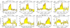 |
Fig. 1. Single-dish spectra of the CO rotational emission lines in PLCK_G244.8+54.9 observed with EMIR. The continuum-subtracted and binned spectra were fitted with two Gaussian components using the CLASS package of GILDAS, by fixing the peak velocities to those measured on the CO(3–2) spectrum. The best-fit line profiles are plotted as red curves, with the individual spectral components overlaid in gray. Velocity offsets are defined relative to the best spectroscopic redshift z = 3.0054 ± 0.0001 presented in Table 1. The resulting line properties are listed in Table A.2 and EMIR spectra of other Planck’s dusty GEMS are shown in Appendix A. |
Furthermore, the CO(1–0) transition in five of the GEMS was observed with the Green Bank telescope (GBT) by Harrington et al. (2018). We will discuss the impact of including the measured line fluxes in our analysis of the CO gas excitation and the implications for the number of molecular gas phases in these intense starbursts, under the assumption that relative flux calibrations between IRAM and GBT spectra are reliable and that the differences in beam sizes play a minor role.
3. Characterizing the CO line emission
We now present our results on the properties of the star-forming gas reservoirs in the GEMS, through searching for the peak of the CO ladder and the characterization of the spatially-integrated CO line ratios.
3.1. CO line profiles of individual sources
By combining all observing runs, we detected 45 CO lines with Jup ≥ 3 out of the 48 observed lines, and up to high rotational levels (maximum of Jup = 11) that trace the warm and dense regime of the bulk of the molecular gas. Our data set includes between two and eight CO lines per source. We fitted each baseline-subtracted and coadded spectrum using a Gaussian function and measured the central frequencies of the lines, as well as the redshifts, full-widths-at-half-maximum (FWHM), and velocity-integrated fluxes. Results are reported in Table A.2, together with the uncertainties provided by the CLASS fitting routine. Line fluxes are uncorrected for lensing magnification. Seven out of the 11 GEMS exhibit single Gaussian profiles and we only use a double Gaussian for PLCK_G045.1+61.1, PLCK_G092.5+42.9, PLCK_G145.2+50.9, and PLCK_G244.8+54.9, where this additional spectral component is robustly detected (see Figs. 1, A.1–A.3).
We computed flux upper limits for the lines without 3σ detections following the approach adopted in Rowlands et al. (2015). We obtained a broad range of line FWHM values, from 200 to 750 km s−1, similar to lensed and unlensed SMGs in the literature (see also C15), and very high fluxes up to 37 Jy km s−1, uncorrected for gravitational magnification. The best spectroscopic redshifts of each source listed in Table 1 were measured from single Gaussian fits to the two lowest-J CO lines detected with EMIR, typically either Jup = 3 and 4 or Jup = 4 and 5.
3.2. CO spectral line energy distributions
Figure 2 shows the individual CO SLEDs of the 11 GEMS, in units of velocity-integrated flux densities. This plot demonstrates that our survey covers the peak of the SLED for nine out of 11 sources, and that this peak systematically falls between Jup = 4 and Jup = 7. This is crucial to shed light on the gas conditions in the GEMS, since the location of the maximum on the CO excitation ladder directly depends on the gas kinetic temperature and density. For this reason, the only two CO transitions detected in PLCK_G145.2+50.9 and the flat ladder of PLCK_G113.7+61.0 in the range Jup = 4–8 will, to a certain extent, prevent us from deriving detailed gas properties in these sources. The SLEDs of PLCK_G092.5+42.9 and PLCK_G244.8+54.9, the two brightest GEMS with well-sampled SLEDs up to Jup = 10–11 exhibit double peaks that strongly suggest the presence of two distinct gas excitation components. We provide further evidence of these multiple gas phases using detailed excitation models in Sect. 5.
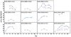 |
Fig. 2. CO spectral-line energy distributions of the Planck’s dusty GEMS. Blue triangles show the velocity-integrated line fluxes uncorrected for gravitational magnification, as measured in this work with EMIR on the IRAM 30-m telescope. All CO(1–0) fluxes are taken from Harrington et al. (2018, black triangles) and CO(3–2) for PLCK_G092.5+42.9 is from Harrington et al. (2016). For PLCK_G045.1+61.1, PLCK_G092.5+42.9, and PLCK_G244.8+54.9, light blue and red triangles show the SLEDs obtained for the blue and red kinematic components, respectively, for the transitions with S/N values sufficiently high to obtain a robust separation of the two components. |
We also determined the shape of the SLED for individual “blue” and “red” components (named according to their position relative to the systemic redshifts of Table 1) in PLCK_G045.1+61.1, PLCK_G092.5+42.9 and PLCK_G244.8+54.9, the three GEMS where two spectral components are detected over several CO lines. To obtain a robust separation, we fixed the central velocities of the individual components to those measured on the lowest-J transition with the highest S/N value, typically either CO(3–2) or CO(4–3) (see Table A.2). The two Gaussians are centered at about –420 and 30 km s−1, –120 and 170 km s−1, –210 and 150 km s−1 (with respect to the spectroscopic redshifts of Table 1) for PLCK_G045.1+61.1, PLCK_G092.5+42.9 and PLCK_G244.8+54.9, respectively. Varying only the FWHM and peak flux of each kinematic component enables us to properly fit the profiles of all mid- and high-J lines, apart from the CO(11–10) transition in PLCK_G244.8+54.9, which has a lower S/N value. The spectral components in PLCK_G244.8+54.9 illustrated in Fig. 1 have central velocities consistent with those of the two regions identified in Cañameras et al. (2017a) from ALMA 0.1″-resolution imaging of the CO(4–3) line emission. The resulting CO SLEDs for the blue and red kinematic components are shown in Fig. 2. For PLCK_G045.1+61.1, both SLEDs are very similar to the one derived from integrated CO fluxes, and peak at Jup = 5. In PLCK_G092.5+42.9, the measured fluxes of the blue component are nearly constant between Jup = 4 and Jup = 8, implying that the variations of the global SLED are mainly driven by the red component. The relative gas excitation in PLCK_G244.8+54.9 is less obvious, with the red component having a larger contribution to the main peak. We further investigate their individual properties in Sect. 5.1.
The relative variations between sources are shown in Fig. 4 by plotting the CO SLEDs normalized by the CO(3–2) velocity-integrated fluxes. We also show how the GEMS compare with other well-studied starburst galaxies in the literature, such as the local starburst Arp 220 (Wiedner et al. 2002; Rangwala et al. 2011), the central region of M 82 (Weiß et al. 2005), and the Cosmic Eyelash (Danielson et al. 2011). Overall, the variety of CO ladders is consistent with the wide range of CO excitations found over the SMG population (Casey et al. 2014). The CO ladder of the most excited GEMS, the Ruby, peaks at Jup = 6, similarly to the local starburst M 82 (Fig. 4). This is in line with the detailed analysis of Cañameras et al. (2017a), which showed that star-forming regions within this maximal starburst could resemble the densest inner parts of molecular regions within low-redshift galaxies.
The CO(1–0) fluxes are comparatively higher than those from local starbursts, assuming that the relative flux calibrations between our CO line survey with EMIR and GBT observations from Harrington et al. (2018) have uncertainties of up to ∼30%. This suggests that the GEMS host a low-excitation gas component distinct from the excited gas phases, as further discussed in Sect. 5.2. Moreover, the fact that the SLED of the most excited sources in the sample peak at Jup ≤ 6, and compare well with the gas excitation in Arp 220, provides further evidence that the GEMS are intense starbursts that do not host a powerful AGN (see, in contrast, the turnover at Jup = 10 for the z = 3.9 QSO APM 08279, Weiß et al. 2007; Bradford et al. 2011). We constrain the maximal contribution from an X-ray dominated region to the overall gas heating in Sect. 6.3.
Sources in local thermal equilibrium (LTE) with thermalized CO rotational levels exhibit SLEDs rising as the square of Jup. Figure 4 shows that only PLCK_G092.5+42.9, PLCK_G102.1+53.6, and PLCK_G244.8+54.9 have CO transitions nearly in thermal equilibrium up to Jup ∼ 4, consistent with the presence of subthermally excited reservoirs, as also found, for example, in Harris et al. (2010).
3.3. CO line luminosities
To quantify the total energy radiated by each CO transition we converted the fluxes to line luminosities, in L⊙, using the relation from Solomon et al. (1992):
 (1)
(1)
where Iline is the velocity-integrated flux in Jy km s−1, νobs the observed frequency of the line in GHz and DL the luminosity distance in Mpc. We also computed line luminosities in K km s−1 pc2 using:
 (2)
(2)
All observed line luminosities (uncorrected for the gravitational magnification) are reported in Table A.2.
In Fig. 3, we plot the relations between LFIR and  for all CO transitions detected in at least one GEMS, and the best-fitting linear relations obtained for local galaxies and individual star-forming regions (Liu et al. 2015) as well as for low-redshift ULIRGs only (Kamenetzky et al. 2016). The two low-redshift comparison samples cover FIR luminosities up to about 1012L⊙. Moreover, ULIRGs span a particularly small dynamical range of less than two orders of magnitude in luminosity, which leads to differences in the high-JLFIR–
 correlations between both samples, although the measured slopes appear to be consistently sublinear (e.g., Greve et al. 2014; Kamenetzky et al. 2016). The GEMS closely follow the low-redshift correlations from Liu et al. (2015) and cover the same regime as other samples of high-redshift dust-obscured star-forming galaxies (Yang et al. 2017). When comparing to local ULIRGs, the CO transitions with Jup ≥ 5 that are thought to arise from the denser and warmer gas components directly related to the on-going star-formation activity appear to best follow the local trends. For Jup ≤ 4, the lower number of sources available in the catalog of Kamenetzky et al. (2016) results in more scattered relations, which complicates the interpretation.
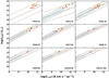 |
Fig. 3. Relations between LFIR and |

We derived the spatially-integrated CO line luminosity ratios for the five GEMS with both CO(1–0) (from Harrington et al. 2018), and mid-J flux measurements, finding r32/10 = 0.42 ± 0.04, r43/10 = 0.30 ± 0.05 and r54/10 = 0.22 ± 0.05. These values are 20–30% lower than ratios obtained in Bothwell et al. (2013) for unlensed SMGs. The r32/10 ratio has been particularly well constrained for high-redshift dusty star-forming galaxies, with measurements in the range r32/10 = 0.40–0.65 (Harris et al. 2010; Tacconi et al. 2010; Carilli & Walter 2013; Greve et al. 2014; Genzel et al. 2015; Daddi et al. 2015; Sharon et al. 2016; Yang et al. 2017), and our estimate therefore remains consistent with the typical values found in the literature. We further interprete these line ratios in terms of gas phases following our gas excitation analysis in Sect. 5.2.
4. Global gas properties of the GEMS
4.1. Correcting for the lensing magnification
4.1.1. Magnification factor estimates
For each source, we used our best-fitting lens model with LENSTOOL (Jullo et al. 2007) to derive amplification maps with the same sampling as the subarcsec resolution CO line and dust continuum maps from our SMA, PdBI, and ALMA follow-up interferometry. The details of our lens modeling approach are described, for example, in Cañameras et al. (2017b) and Cañameras et al. (2018). We then used these maps to compute the luminosity-weighted gravitational magnification factors of the gas and dust components, in order to correct the observed velocity-integrated CO fluxes and line luminosities. We accounted for the frequency variations of the beam size by using the following parametrization of the observed half-power beam width2 (HPBW): HPBW/[arcsec]=2460 × (ν/[GHz])−1. We only considered pixels where the CO line or dust continuum emission is detected above 4σ, and we rejected a small fraction of 5–10 pixels that lie on top of the critical lines and have artificially high magnification factors above 200.
Table 1 summarizes the resulting magnification factors for each source and their 1σ statistical uncertainties. The luminosity-weighted magnification factors of the gas component were inferred from our high-resolution line imaging with the PdBI, for mid-J CO transitions between Jup = 4 and Jup = 6. Unless otherwise stated, for the cold dust component we used SMA continuum maps at 880-μm either in the EXT or VEXT configuration, at similar beam size as our PdBI observations. The CO maps of PLCK_G092.5+42.9, PLCK_G102.1+53.6, and PLCK_G231.3+72.2 have significantly lower resolutions than those from the SMA, and we computed μdust from the 2-mm dust continuum extracted in line-free baseline channels from the PdBI data cubes to avoid beam effects on the magnification factor estimates. We also quote the systematic errors on μ induced by the choice of the mass profile of the main deflector or the inclusion of photometrically-selected multiple image systems, as inferred from the alternative models that will be further discussed in a forthcoming paper (Cañameras et al., in prep.). The luminosity-weighted magnification factors of the Ruby were computed within the beam of the 30-m telescope in the same way as for the other GEMS, based on the detailed lensing analysis of Cañameras et al. (2017b) that shows local variations of μ by up to a factor of 2 for individual clumps in this source.
PLCK_G200.6+46.1 and PLCK_G138.6+62.0 are the only unresolved sources in our follow-up submm interferometry of the whole sample. The main lens galaxies in these systems also lack spectroscopic redshift measurements, which precludes the calculation of detailed lensing models. Since most results rely on line ratios, we nonetheless included these GEMS in the overall analysis and used their position in the LFIR–Tdust parameter space relative to the sequence of unlensed SMGs to derive their gravitational magnification (see Fig. 5 and justification in C15). This method, although crude, provides estimates of μ which are within 25% of the magnification factors obtained from detailed modeling for six sources (Table 1), and within a factor 2 for the remaining three.
4.1.2. Constraints on the differential magnification
Previous studies have cautioned that differential magnification effects can become an important source of systematic uncertainties when characterizing the molecular gas properties of strongly lensed dusty star-forming galaxies (e.g., Blain 1999). This effect can play an important role when comparing fluxes from mid-J CO lines with CO(1–0) because these transitions have critical densities varying by 1–3 orders of magnitude and therefore trace different gas components in the sources. Jup > 2 CO lines trace warm molecular regions which are expected to be compact in high-redshift starbursts, under the form of late-stage mergers akin to the nucleus of Arp 220 (Scoville et al. 2017) or massive star-forming clumps distributed over gas-rich disks (e.g., Swinbank et al. 2010; Thomson et al. 2015), while CO(1–0) is thought to arise from the cool and more diffuse ISM (e.g., Ivison et al. 2011). When observing strongly lensed galaxies, one of these components can benefit from a higher gravitational magnification, depending on the position of the source plane caustic lines. Simulations showed that uncertainties on the CO(6–5)/CO(1–0) line flux ratio due to differential magnification can reach up to 30% (Serjeant 2012) and therefore distort the observed CO SLEDs, but the amplitude of this effect essentially depends on the actual distribution of the low and high-excitation gas phases in these systems. We quantified differential magnification over the sample using two different approaches.
Firstly, we used our detailed lensing models to quantify the level of differential lensing between mid-J CO lines and dust continuum of individual Planck’s dusty GEMS. IRAM/PdBI and ALMA subarcsec resolution line-imaging constrain the morphology of the CO line emission in all sources and allow us to compare with the resolved dust continuum maps to search for variations of the luminosity-weighted magnification factors between the two components. The results of Table 1 demonstrate that values of μgas and μdust are within 1σ for PLCK_G080.2+49.8, PLCK_G102.1+53.6, PLCK_G165.7+67.0 and PLCK_G244.8+54.9, and differ by at most 15–30% for other sources. These variations are comparable with other measurement uncertainties, including IRAM flux calibration uncertainties, and might be partly due to residual differences in the beam dimensions of about 20% (e.g. for PLCK_G045.1+61.1 and PLCK_G092.5+42.9), despite our efforts in computing the luminosity-weighted magnification factors at similar angular resolutions.
The simulation study presented in Serjeant (2012) suggests that differential magnification effects between [C II] and FIR bolometric emissions are minor, for ISM configurations resembling that of the Cosmic Eyelash. [C II] and CO(1–0) line emissions also present similar magnifications. This suggests that if the sources have configurations similar to the Cosmic Eyelash, which is broadly supported by our multiwavelength analysis of PLCK_G165.7+67.0 (Cañameras et al. 2018), the μdust value can serve as a proxy for the magnification of the low-density CO(1–0) gas reservoirs. Under these assumptions, our high-resolution interferometry therefore suggests that differential lensing effects between CO(1–0) and mid-J CO lines are minor in this sample. The effect is most likely negligible between mid- and high-J CO transitions that both trace the compact sites of star formation, as demonstrated by Rybak et al. (2015) for the well-studied dusty starburst SDP 81.
Secondly, we compared the CO line profiles from our IRAM survey to show that differential lensing is not producing a significant bias between different rotational levels. Values given in Table A.2 show that for each source, most line FWHMs measured with single component Gaussian fits are within the 1σ uncertainties, suggesting that Jup > 3 transitions consistently trace the same intrinsic gas kinematics. For PLCK_G045.1+61.1, PLCK_G092.5+42.9, PLCK_G145.2+50.9, and PLCK_G244.8+54.9, we also detect the same number of spectral components from Jup = 3 to Jup = 10, on the transitions with sufficient signal-to-noise ratios (Fig. 1, A.1–A.3). More puzzling is the line profile of CO(6–5) in PLCK_G092.5+42.9, where the two spectral components are robustly detected but with very different flux ratios compared to other transitions. However, since the profiles of CO(8–7) and CO(9–8) lines in this source are consistent with those of CO(4–3) and CO(5–4), we conclude that different gas excitation properties within the blue and red components are more likely to produce different flux ratios on a single transition than differential lensing effects. For these reasons, we assumed that differential lensing is not likely to induce major distortions of the CO SLEDs and hence we ignored this effect for the gas excitation analysis.
4.2. The αCO conversion factor
Deriving the molecular hydrogen masses of the GEMS from our analysis of the CO gas excitation relies on our assumption about the αCO conversion factor, which can induce major uncertainties in high-redshift studies despite the overall consensus reached for local galaxy populations (see Bolatto et al. 2013). However, the 3P1–3P0 fine-structure line of atomic carbon has also proven to be a reliable proxy of the total molecular gas content in galaxies. Due to its low critical density (ncrit ≃ 500 cm−3, Carilli & Walter 2013) it is easily thermalized in molecular clouds and originates from the extended and low-density gas reservoirs that contain the bulk of the molecular gas mass, similarly to CO(1–0), both in nearby (e.g., Papadopoulos et al. 2004; Jiao et al. 2017) and high-redshift ULIRGs (e.g., Alaghband-Zadeh et al. 2013). We can therefore invert the problem by using the detailed analysis of atomic carbon in the GEMS from N18 to derive αCO for the seven sources with [C I](1–0) line detections with EMIR, assuming that it traces the same gas components as CO(1–0).
For these seven GEMS, we used the [C I]-inferred H2 masses from N18, obtained with the relation from Papadopoulos et al. (2004) (see also Eq. 2 in Wagg et al. 2006) and for a common value of the carbon abundance, X[CI] = 3 × 10⁻⁵ (Weiß et al. 2005), an excitation factor, Q10 ≃ 0.5, and the Einstein coefficient, A10 = 7.93 × 10⁻⁸ s−1. We then used the CO(1–0) line luminosities,  , either measured in Harrington et al. (2018) or converted from the mid-J transitions detected with EMIR using the average r32, 10 and r43, 10 conversion factors measured over the sample in Sect. 3.3. Comparing M[CI] (H2) and
  results in the values of αCO shown in Table 2 and Fig. 5. For all but one source, we obtain low conversion factors consistent within 1σ with αCO ∼ 0.8 M⊙ (K km s−1 pc2)−1, the value measured for local ULIRGs and widely used for luminous dusty starbursts at high redshift (see also Bolatto et al. 2013). PLCK_G080.2+49.8 is the only GEMS for which we measure a higher conversion factor inconsistent with the ULIRG value, which is perhaps not surprising since the local star-formation properties within this source are more akin to high-redshift main-sequence galaxies than other extreme starbursts in our sample (N18).
Estimates of the CO-to-H2 conversion factors, gas masses and gas-to-dust ratios.
These results are nevertheless strongly dependent on our choice of the carbon abundance. Enhanced abundances with respect to those over the Galactic plane have been measured in high-redshift starbursts (X[CI] ≃ 4−5 × 10⁻⁵, Weiß et al. 2005; Danielson et al. 2011; Alaghband-Zadeh et al. 2013). We refer to N18 for a discussion of the physical origin and implications of a possible enhanced carbon abundance in the GEMS, and emphasize that this would lower our estimates of αCO and favor the use of a low ULIRG-like factor. Given these considerations, in Sect. 5.2 we therefore take a common factor of 0.8 M⊙ (K km s−1 pc2)−1 to convert the CO line luminosities of the 11 sources to gas masses. This is in line with results obtained in C15 from dust mass measurements and assuming solar-like metallicities. Moreover, Fig. 5 illustrates that this choice is also consistent with independent estimates for other strongly lensed SMGs in the literature (e.g., Aravena et al. 2016).
5. Properties of the CO gas excitation
We now further investigate the CO excitation within each of the GEMS and deduce the physical gas properties using two independent radiative transfer analyses that rely either on the entire SLEDs or a range of measured CO line ratios.
5.1. Large velocity gradient models
5.1.1. Modeling approach
The large velocity gradient (LVG) approach (e.g., Young & Scoville 1991) is commonly used to model the molecular gas excitation in galaxies having optically thick gas reservoirs that are not thermalized, as is the case for the GEMS (see Fig. 4). LVG models can predict the shape of the CO ladder by computing the collisional excitation of CO molecules for a range of gas physical conditions, assuming that turbulent motions within star-forming clouds result in velocity gradients in order to compute the escape probability of optically thick CO emission. We derived radiative transfer LVG models for the GEMS using the Markov chain Monte Carlo (MCMC) implementation of RADEX (van der Tak et al. 2007) presented in Yang et al. (2017)3. This one-dimensional code assumes spherical symmetry and describes the velocity gradients, dv/dr, in the expanding sphere approximation. It performs an MCMC sampling of the parameter space that includes the molecular hydrogen density, nH2, the gas kinetic temperature, Tk, the CO column density per unit velocity gradient, NCO/dv, and the size of the emitting region, and samples the posterior probability distributions functions from the CO line fluxes modeled by RADEX.
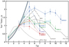 |
Fig. 4. Observed CO SLEDs normalized by the CO(3–2) line fluxes for the GEMS with CO(3–2) detections (the CO(1–0) fluxes are from Harrington et al. 2018), the local starburst Arp 220 (Wiedner et al. 2002; Rangwala et al. 2011), the central region of M 82 (Weiß et al. 2005) and the Cosmic Eyelash (Danielson et al. 2011). For comparison, we also show the CO SLED spatially-integrated over the inner disk of the Milky Way (dotted line, Fixsen et al. 1999), and the expected trend for optically thick gas in local thermodynamic equilibrium (thick gray line). |
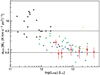 |
Fig. 5. CO luminosity to gas mass conversion factor, αCO, versus FIR luminosity, for the seven Planck’s dusty GEMS with direct αCO measurements using the molecular gas masses inferred from the [C I](1-0) line fluxes of Nesvadba et al. (2018, red stars). All but one GEMS are consistent with the usual ULIRG value αCO = 0.8 M⊙ (K km s−1 pc2)−1 (lower dashed line). Other points show αCO estimates in the literature, for the strongly lensed SMGs from the SPT survey (blue points), high-redshift unlensed dust-obscured starbursts (green points), QSOs (yellow points) and main sequence galaxies (black squares, Aravena et al. 2016, and references therein). The relative uncertainties on αCO obtained for these high-redshift samples are comparable to those of the GEMS. |
Following the CO excitation analysis of strongly-lensed SMGs from the H-ATLAS survey presented in Yang et al. (2017), we assumed flat prior probabilities for the input parameters within the following ranges: nH2 = 101.5–107.0 cm−3, Tk = TCMB − 103 K and NCO/dv = 1015.5–1019.5 cm−2 km−1 s. Here TCMB is the CMB temperature at the redshift of the source (see further justifications and references in Yang et al. 2017). The size of the CO-emitting region is also a free parameter in RADEX that acts as a normalization factor on the overall SLEDs, but the size estimates from the LVG models are quite uncertain given the dependency on both the magnification factor and the beam filling factor. We therefore refer to Sect. 6 for a dicussion of the physical extent of the molecular gas reservoirs and mainly discuss the best-fitting values of nH2, Tk and NCO/dv that fully determine the shape of the SLEDs.
For each source, we sampled the posterior probability distribution functions using 1000 MCMC iterations. As an example, we show the one-dimensional and joint two-dimensional posteriors of each parameter for PLCK_G244.8+54.9 in Fig. 6. The best-fitting values of nH2, Tk and NCO/dv are taken from the maximum of the joint probability distribution and are listed in Table 3 together with 1σ uncertainties. We also plot the modeled CO SLEDs from the best-fitting estimates of the gas densities and kinetic temperatures together with our CO flux measurements with EMIR in Figs. 6, B.1, and B.2.
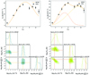 |
Fig. 6. Top left: observed CO SLED of PLCK_G244.8+54.9, the Ruby (black points), without correcting the velocity-integrated fluxes for gravitational magnification. The orange line shows the best-fit model with RADEX using a single gas excitation component, and illustrates a case where this simple model poorly reproduces the CO ladder for Jup ≳ 6. Top right: best-fit model from RADEX using two gas excitation components (solid orange line). The dot-dashed orange line shows the low excitation component, which is assumed to be cooler and more extended than the high excitation component (dashed yellow line) in the analysis. Bottom: one-dimensional and joint two-dimensional posterior probability distributions of nH2, Tk and NCO/dv, obtained from our MCMC sampling of the RADEX parameter space in the two-component model, for the low (left) and high (right) excitation components. Contours increase in steps of 0.5σ. Yellow and orange solid lines show the maximum posterior probability of each parameter, while dotted lines mark the ±1σ range in the distributions. The resulting parameter values are listed above the corresponding histograms. |
Molecular gas properties of the Planck’s dusty GEMS inferred from the MCMC sampling of the LVG model parameter space using RADEX.
5.1.2. Integrated physical properties
The well-sampled mid-J regime of the CO SLEDs provides robust constraints on the gas density and temperature for all GEMS. For a single gas excitation component, we obtain molecular hydrogen densities ranging between 102.6 and 104.1 cm−3, gas temperatures log(Tk)=1.5–3.0 K and NCO/dv = 1016 − 17.5 cm−2 km−1 s. These conditions are very similar to those within high-redshift SMGs from the H-ATLAS sample (Yang et al. 2017) and cover the same density and temperature regimes as local ULIRGs, whose CO ladders also peak between Jup = 4 and Jup = 7 (e.g., Weiß et al. 2005; Rosenberg et al. 2015).
The CO(1–0) line emission in high-redshift dusty star-forming galaxies may have contributions from gas components not seen in the mid-J CO lines (e.g., Ivison et al. 2010), and this transition appears to be a good proxy of the extended and low-density molecular gas reservoirs that are not directly related to star formation. We reproduced the single-component analysis without the CO(1–0) fluxes in order to determine how the gas density and kinetic temperature are affected by this transition and to avoid the difficulty of constraining possible differential lensing effects between Jup = 1 and higher-J transitions. The comparison shown in Fig. 7 only indicates minor differences in the inferred molecular gas properties, suggesting that this single data point can not bias the fit of our SLEDs, well-sampled between Jup = 3 and Jup = 7.
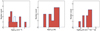 |
Fig. 7. Results of the gas excitation analysis with RADEX. Red histograms show the median values of the marginal probability distributions of nH2, Tk and NCO/dv obtained by modeling the CO SLEDs with a single excitation component (see Table 3). Blue histograms illustrate how results change when removing the CO(1–0) fluxes from the analysis. |
In some cases our simple one-component model poorly reproduces the CO ladder. For example, a significant discrepancy is found at Jup ≥ 6 for PLCK_G244.8+54.9 (Fig. 6), and both the CO(1–0) and Jup > 7 fluxes are underestimated for PLCK_G092.5+42.9 and PLCK_G113.7+61.0 (Fig. B.1). This suggests that the CO SLEDs in those GEMS trace at least two gas phases with distinct physical properties, an extended and cold gas phase with low excitation and the more compact and warmer gas reservoirs with higher excitation. Previously, several studies also used multicomponent LVG models to adequately describe the CO excitation, both at low (e.g., Weiß et al. 2005) and high redshift (e.g., Daddi et al. 2015), including for distant obscured starbursts (e.g., Danielson et al. 2011; Hodge et al. 2013; Yang et al. 2017). Obtaining reliable detections of low-excitation gas phases in SMGs remains nonetheless challenging because this component is intrinsically weaker than in local normal star-forming galaxies (Rosenberg et al. 2015), and because spatially-integrated CO SLEDs are sensitive to luminosity-weighted parameters and therefore dominated by the less massive, but highly excited dense gas reservoirs (Kamenetzky et al. 2018). The CO SLEDs of a majority of six out of 11 GEMS are not sufficiently sampled to identify such multiple gas phases.
We used two-excitation component models with the same approach, and assigned different parameters to each excitation component within common physical boundaries. Most importantly, the model assumes two additional priors on the relative sizes and temperatures within the Bayesian analysis, requiring that the low-excitation gas component is cooler and more extended than the high-excitation component (as supported by multi-J CO observations in SMGs, Ivison et al. 2011; Casey et al. 2014). For PLCK_G092.5+42.9 and PLCK_G244.8+54.9, the presence of the two gas phases with different levels of excitation is highlighted by the two apparent peaks and the best-fitting solution from the two-component model provides a much better fit to the overall SLED (see Figs. 6 and B.1). The two components are also apparent in PLCK_G113.7+61.0, PLCK_G138.6+62.0, and PLCK_G165.7+67.0, where the single-component model significantly underestimates the CO(1–0) and CO(3–2) fluxes (see Fig. B.1). The overall SLEDs of these sources are nevertheless nearly constant up to Jup = 6 and dominated by the excited gas phase. For this reason we checked that the second lower excitation phase is also detected after removing the CO(1–0) lines from the analysis, and found that the CO(3–2) fluxes remain underestimated by the new models. We therefore conclude that the detection of multiple gas phases in PLCK_G113.7+61.0, PLCK_G138.6+62.0, and PLCK_G165.7+67.0 is robust and that the properties of the low excitation component inferred with and without the CO(1–0) fluxes are consistent within 1σ.
Our two-component models favors low-excitation gas phases peaking between Jup = 2 and 5, while the high-excitation components peak at higher J and consequently have elevated densities and temperatures (best-fitting results summarized in Table 3). For PLCK_G092.5+42.9 and PLCK_G244.8+54.9, the high excitation component even reaches  and
and  , for kinetic temperatures of about 70 and 200 K, respectively. In these two sources, the cooler and more extended gas phase covers the main peak at Jup = 4–6 and is thereby significantly excited, with conditions similar to those of the highly excited gas phase in the Cosmic Eyelash (Danielson et al. 2011), or to the bulk of the gas reservoirs in low-redshift compact ULIRGs and nearby starbursts (e.g., Bradford et al. 2003). Interestingly, for PLCK_G113.7+61.0, PLCK_G138.6+62.0, and PLCK_G165.7+67.0, the best-fitting lower excitation component peaks at Jup = 2–3, similarly to the CO SLEDs observed for the inner Galactic disk (as illustrated in Fig. 4, Fixsen et al. 1999) or local spirals (e.g., Braine & Combes 1992). We measure molecular hydrogen densities of about 102.8 and 102.4 cm−3 for PLCK_G113.7+61.0 and PLCK_G138.6+62.0, respectively, suggesting that this Milky Way-like component is diffuse and might trace extended gas reservoirs not directly fueling star formation, as already postulated for other high-redshift dusty starbursts (e.g., the Cosmic Eyelash, Danielson et al. 2011).
5.1.3. Individual spectral components
We used the spectral component separation described in Sect. 3.2 and the individual CO SLEDs shown in Fig. 2 to study the variations of the gas excitation within each kinematic component. The new LVG models were derived using the same approach and the same number of gas excitation components as for the spectrally-integrated CO spectra (see Fig. B.3). The best-fitting models were then extrapolated down to low-J to predict CO(1–0) fluxes and derive gas masses for the blue and red components, assuming αCO = 0.8 M⊙ (K km s−1 pc2)−1 (see Table 2).
For PLCK_G045.1+61.1, the two modeled CO SLEDs peak between Jup = 4 and Jup = 5 similar to that obtained for the global spectra in Fig. B.2. The density and temperature of the single gas excitation components are therefore consistent, within the uncertainties, with  and
and  , as measured on the overall SLED. Comparing the CO(1–0) fluxes extrapolated from the best-fitting models shown in Fig. B.3 with those extrapolated from the LVG models of the overall SLED (Fig. B.2) suggests that the blue and red components each comprise about half of the total gas mass in PLCK_G045.1+61.1.
The two spectral components in PLCK_G092.5+42.9 also exhibit similar levels of excitation, including a cool and extended gas phase peaking at Jup = 3–5 and a warmer and more compact phase producing a secondary peak at Jup = 7–9. The red kinematic component more closely resembles the global SLED and strongly peaks at Jup = 4–5, although the flux drop measured for the CO(6–5) transition is affected by large uncertainties on the component separation, and possibly by differential magnification effects (see discussion in Sect. 4.1.2). Its properties are fully consistent with the best-fit parameters of Table 3. The kinetic temperatures of the blue kinematic component are also similar and its densities are  and
and  for the low and high-excitation phases, respectively, which is somewhat lower, but consistent within 1σ with those measured on the overall SLED. Models of the blue and red components extrapolated to Jup = 1 show that they contain about 30% and 20% of the gas mass inferred from the CO(1–0) line detection, respectively, suggesting that gas components not seen in mid-J CO lines also contribute to the CO(1–0) fluxes.
In PLCK_G244.8+54.9, the two components have comparable amplitudes over the entire SLED, and the CO(1–0) fluxes extrapolated from the two-component gas excitation models suggest that they contain similar gas masses. The properties of the red component are consistent with those listed in Table 3. However, the SLED of the blue component rises from Jup = 8 to Jup = 10, which given the large uncertainties, provides marginal evidence that the warm gas phase in the blue component is more excited, with molecular gas densities about one order of magnitude higher than those determined from the integrated SLED.
5.2. CO-inferred molecular gas masses
Detailed modeling of well-sampled CO SLEDs provide robust estimates of the molecular gas masses from mid-J CO lines. The measured CO line luminosities can be converted to those of CO(1–0),  , and to the total molecular hydrogen masses, MCO(H2), using the best-fitting CO excitation models and the relation
  . For the 11 Planck’s dusty GEMS, we extrapolated the best-fitting LVG models inferred exclusively from the Jup > 3 CO flux measurements, and predicted the CO(1–0) fluxes and total masses of gas embedded within these excited reservoirs, directly related to the on-going star formation. This method does not include the possible additional contribution from diffuse ISM components extended over roughly kpc scales and spatially segregated from the excited gas phases that have already been detected in some SMGs (see e.g., Harris et al. 2010), and it is not strongly sensitive to differential magnification since this effect is not significantly affecting the overall shape of the CO SLEDs (see Sect. 4.1.2). We used the two-excitation components model for the five sources with CO SLEDs that are poorly fit by a single combination of nH2 and Tk, and the single-component model for the six others (see Figs. B.1 and B.2). The predicted CO(1–0) fluxes were then converted into line luminosities and molecular hydrogen masses using αCO = 0.8 M⊙ (K km s−1 pc2)−1, following the discussion in Sect. 4.2.
We obtain the total gas masses listed in Table 2, which are spatially-integrated over the source components falling within the beam of the IRAM 30-m telescope and corrected for the gravitational magnification factors, μgas, of Table 1. MCO(H2) broadly ranges between 1010 and 1011 M⊙, with a mean value of 4.3 × 10¹⁰ M⊙, akin to the masses obtained for other samples of lensed or unlensed high-redshift SMGs with single-dish CO(1–0) detections or well-sampled CO SLEDs (e.g., Harris et al. 2012; Bothwell et al. 2013). This shows that the GEMS have global gas contents comparable with the overall SMG population, despite being extremely bright on the sky due to their strong gravitational magnifications. PLCK_G145.2+50.9 is almost a factor two more massive than other sources in the sample, suggesting that this is an extremely gas-rich starburst or that our estimate of the magnification factor may be too low, for example due to the presence of large-scale structures at different redshifts along the line of sight. The best-fitting models in Figs. 6 and B.1 indicate that the low-excitation component dominates the overall mass budget in PLCK_G092.5+42.9, PLCK_G113.7+61.0, PLCK_G138.6+ 62.0, and PLCK_G244.8+54.9, while the mass of both components are comparable in PLCK_G165.7+67.0. For these five sources, the molecular gas masses would be systematically lower if we had used the single component models instead.
We then used the dust masses from SED fitting in C15 and the luminosity-weighted magnification factors of the dust continuum, μdust, presented in Table 1, to infer the global gas-to-dust mass ratios, δGDR (see Table 2). We obtained an average gas-to-dust mass ratio of about 150 over the sample, consistent with other high-redshift SMGs (e.g., Ivison et al. 2011) and local ULIRGs (e.g., Solomon et al. 1997).
The best-fitting RADEX models of the CO Jup ≥ 3 ladder systematically underestimate the CO(1–0) fluxes for the five sources detected with the GBT in Harrington et al. (2018), regardless of our assumption of the number of excitation components. If this reflects the intrinsic ratio of the gas mass probed in these transitions, then it implies that some of the Planck’s dusty GEMS contain low-density gas reservoirs segregated from the excited components traced by the mid- to high-J CO lines observed with EMIR. As discussed above, Figs. 6 and B.1 show that the cooler gas phase in the two-component LVG models of PLCK_G092.5+42.9, PLCK_G165.7+67.0, and PLCK_G244.8+54.9 is still significantly excited, with peaks in the range Jup = 3–5 implying molecular gas densities of 103–104 cm−3. This suggests that these GEMS might not only contain the two excited gas phases with different conditions, but also additional reservoirs of gas with lower levels of excitation that are not currently included in the analysis and would explain the excess of CO(1–0) emission. Assuming that the differences between the measured CO(1–0) fluxes and those predicted by the two-component models are indeed associated with such diffuse and low-excitation components, we find that these reservoirs enclose about 20–50% of the total molecular hydrogen mass in PLCK_G092.5+42.9, PLCK_G165.7+67.0, and PLCK_G244.8+54.9. This is comparable with the diffuse mass fraction of 50% measured in the Cosmic Eyelash (Danielson et al. 2011). These fractions would rise up to 80% if we instead assumed the single-component excitation models despite their poor description of the CO SLEDs in the high-J regime.
If the CO(1–0) emission arises partially from gas not probed in the higher-J lines, then differential magnification can be an issue, provided that the relative calibration between the GBT and IRAM observations is robust. Several authors (e.g., Rybak et al. 2015; Spilker et al. 2015) have already pointed out that CO(1–0) line luminosities can have different magnification factors than higher-J CO lines, due to the different spatial distributions of the underlying gas reservoirs. Quantifying this effect would require subarcsec resolution CO(1–0) interferometry. However, we showed in Sect. 4.1 that differential magnification effects between the mid-J CO emission and dust continuum remain below 30%. The excess of CO(1–0) emission observed for these GEMS is also more significant than the upper limit on the differential lensing effect between low- and mid-J CO lines of about 30% predicted by Serjeant (2012), assuming conservatively that the cold and warm CO phases follow very different distributions (thus ignoring massive star-forming disks with well-mixed gas phases). Moreover, attributing the enhanced CO(1–0) emission in the GEMS solely to differential lensing would imply μCO(1 − 0) > μmid-J CO, consistently for all sources. This would correspond to caustic line positions preferentially magnifying the extended low-density regions emitting CO(1–0), with respect to the compact star-forming clouds emitting the bulk of the mid-J CO lines. Although such configurations are not ruled out, for high magnification factors μ ≃ 20, the compact regions are more likely to be more strongly magnified than the extended ones (Hezaveh et al. 2012), which strongly disfavors this interpretation.
For PLCK_G113.7+61.0 and PLCK_G138.6+62.0, the two other GEMS with CO(1–0) measurements, the lower excitation component included in the LVG analysis peaks at Jup = 2–3. This is characteristic of diffuse gas, as already discussed in Sect. 5.1, and includes between 50% and 80% of the total molecular gas mass in the systems, depending on whether CO(1–0) is included in the fit or not. We note that these mass fractions are highly uncertain since the SLEDs are flat in the Jup > 4 regime, which complicates the component separation.
5.3. Photon-dominated region models
In star-forming galaxies, the physical properties and chemical composition of gas clouds affected by the surrounding intense radiation field from the newly formed massive stars have been extensively described by photon-dominated region (PDR) models (e.g., Kaufman et al. 1999; Le Petit et al. 2006; Meijerink et al. 2007). These models are now proposing a coherent picture of the structure of molecular clouds, in the intermediate column density regime between H II regions and prestellar cores, where atomic hydrogen remains neutral and the gas material is predominantly heated by the external FUV field. Atomic carbon is ionized in the outer layers and the CO molecules form deeper within the clouds where the ionizing FUV radiation is sufficiently attenuated (e.g., Hollenbach & Tielens 1997). In this section, we derive simple PDR models to infer the gas densities and the strengths of the incident radiation fields from the spatially-integrated line fluxes.
5.3.1. Method
The PDR diagnostics of the GEMS were derived using the standard one-dimensional models of Kaufman et al. (1999, 2006), which have been widely applied in ISM studies of high-redshift SMGs (e.g., Rawle et al. 2014; Gullberg et al. 2015; Wardlow et al. 2017). We derived the combination of cloud density, nPDR, and FUV radiation field, G0, that best reproduce the observed line luminosity ratios using the PDR TOOLBOX (Pound & Wolfire 2008), a publicly available implementation of the model diagnostics. We followed this approach to infer the physical conditions in the GEMS, under the assumption that they comprise a single giant molecular cloud (Kaufman et al. 1999). Although this simple scenario cannot truly do justice to the intrinsic complexity of the ISM configurations, it allows us to perform a simple and uniform treatment of the integrated properties and to derive the luminosity-weighted, spatially-averaged gas properties. Unlike for the LVG analysis, the average PDR densities are expressed in terms of number densities of hydrogen nuclei and vary in the range 1 < log(nPDR/cm−3) < 7. The strengths of the radiation fields produced by the surrounding young stellar populations (given in units of the Habing field, i.e., 1.6 × 10⁻³ erg cm−2 s−1) are in the range −0.5 < log(G0) < 6.5.
We selected the line ratios that provide complementary constraints on nPDR and G0 and assumed, for a given source, that all spatially-integrated line luminosities arise from a unique PDR that covers the same surface area at all frequencies. High-resolution dust and gas interferometry of high-redshift dusty star-forming galaxies show that this population usually hosts a range of giant molecular cloud complexes (e.g., Thomson et al. 2015) associated with distinct PDRs, as observed in the local Universe, and this approximation therefore implies that the output parameters will be luminosity weighted toward the intrinsically brightest regions.
The CO J/(J − 1) line luminosity ratios essentially constrain the range of gas density in the PDRs, even for the GEMS with high-J CO detections. Diagnostics combining CO and atomic carbon transitions from our companion paper (N18) also lead to degenerate solutions spanning several orders of magnitude in G0. In order to better constrain the gas conditions we therefore included lose constraints from [C II], expected from the ensemble average properties of high-redshift galaxies. In intense starbursts, the bulk of [C II] emission arises from PDRs (e.g., Stacey et al. 2010; Rigopoulou et al. 2014) and, given its low critical density, this line preferentially traces the surface of PDRs. Consequently, line ratios involving [C II] efficiently probe the total energy budget from the external FUV radiation field (e.g., Goldsmith et al. 2012). Since most of the GEMS do not have available [C II] line measurements, we used the distribution of source-integrated [C II] line luminosities measured in Gullberg et al. (2015) for 17 strongly lensed SMGs from the South-Pole Telescope (SPT) survey. We used the average [C II]/FIR luminosity ratio for this sample, which we rescaled to the LFIR values of each GEMS in the rest-frame range 42–500 μm (using the photometry of C15). The resulting [C II] luminosities are consistent with our only available line detection for PLCK_G045.1+61.1, L[CII] ∼ 5.4 × 10¹⁰ L⊙, spatially-integrated over the source components by rescaling the resolved ALMA line luminosity of Nesvadba et al. (2016). We also used the [C I](1–0) line detections with EMIR for some GEMS (N18), and converted the [C I](2–1) line luminosities to [C I](1–0) using the average line ratio over the sample for the sources where the 3P1–3P0 transition of atomic carbon falls outside the observing band.
The best-fitting values of nPDR and G0 listed in Table 4 were inferred from these complementary PDR diagnostics of CO, [C I] and [C II]. We did not distinguish either the different excitation components identified with our LVG models in Sect. 5.1, or the spectral components (as done, for instance, in Rawle et al. 2014), although deblending the PDR properties of individual velocity components within the sources should become feasible by combining the high S/N EMIR CO and [C I] spectra with follow-up [C II] observations. We computed parameter uncertainties using Monte Carlo simulations by randomly drawing each line luminosity from a Gaussian distribution with σ equal to the measurement error, deducing the line ratios and best-fitting values of nPDR and G0 from the PDR diagnostics, and taking the median and 1σ errors on each parameter after 500 iterations.
Best-fitting values of the average number density of hydrogen nuclei, nPDR, and FUV radiation field, G0, obtained for the Planck’s dusty GEMS using the publicly available implementation of the PDR models from Kaufman et al. (1999, 2006).
Line ratios involving CO(1–0) from Harrington et al. (2018) occupy different regions in the nPDR − G0 parameter space than those from mid-J CO, [C I](1–0), and [C II], and point toward FUV radiation fields being systematically lower than ratios involving other species, although CO(1–0) and [C I](1–0) have similar critical densities and should both arise from the outer layers of PDRs. We found that the discrepancy vanishes when using the CO(1–0) luminosities extrapolated from our LVG models, except for PLCK_G165.7+67.0. The multiple solutions obtained for this source might be due to blending of multiple spatial components in the beam of the IRAM 30-m telescope (see more details in Cañameras et al. 2018), or to different distributions of [C I](1–0) and CO(1–0) emission on small scales. Given these uncertainties and hints of distinct low density gas components, we did not consider the single-dish CO(1–0) measurements in the PDR analysis. We also put aside the high-J CO transitions with Jup > 7 that trace the dense molecular gas of n ≳ 105 cm−3 at the inner transition region between the PDRs and molecular clouds, where the external FUV radiation is significantly attenuated and other processes such as cosmic rays could have a major contribution to the gas heating (e.g., Papadopoulos 2010). Furthermore, we verified that the gas densities are well constrained in the process and not dominated by our assumptions on the [C II] line luminosities by reproducing the PDR analysis only with the CO and [C I] line ratios. The resulting values of nPDR are consistent within 1σ with the best-fitting results of Table 4. Finally, we also investigated how the results on G0 would be affected if a significant fraction of the [C II] emission in the GEMS originates outside PDRs, for example from H II regions or diffuse gas reservoirs (Madden et al. 1993; Gerin et al. 2015). For the worst case scenario where non-PDR [C II] emission is about 50% (see also Abel 2006; Decarli et al. 2014), a factor of two decrease in the [C II]/[C I](1–0) luminosity leads to FUV radiation fields that are 0.5–0.7 dex lower than those presented in Table 4.
Recent studies including Bothwell et al. (2017) have advocated the need to account for the influence of cosmic rays on PDR models, since this process becomes an important driver of gas excitation deeply within the molecular clouds shielded from the external FUV radiation (Papadopoulos 2010; Kazandjian et al. 2015). Cosmic ray radiation fields in intensely star-forming galaxies such as the GEMS are expected to be significantly enhanced compared to those in the Milky Way, due to efficient particle acceleration in supernova shockwaves. Bothwell et al. (2017) argue that including this gas heating source is crucial to avoid underestimating the PDR densities. However, quantifying the exact influence of cosmic rays on the gas conditions at high attenuation requires the use of dense gas diagnostics such as line ratios of HCN, HNC, and HCO+, which is beyond the scope of this paper. Here we use ratios of low- to mid-J CO, [C I] and [C II] lines, which are expected to vary little in the presence of enhanced cosmic ray ionization rates in intense starbursts, for sufficiently high surrounding FUV radiation fields (Meijerink et al. 2011). For these reasons, we ignored this heating source during the analysis. Furthermore, we emphasize that modifying other assumptions in the models, for instance on the overall PDR geometry, could affect the resulting PDR densities and FUV radiation fields to a similar extent.
5.3.2. Properties of the PDRs
We followed this approach to infer the best-fitting densities and radiation field strengths of the GEMS within the PDR scenario, and converted these quantities to the corresponding range of PDR surface temperatures using Fig. 2 of Kaufman et al. (1999). All values are presented in Table 4 and Fig. 9. The starbursts cover a small range in gas density, nPDR = 104–105 cm−3, and about two orders of magnitude in external FUV field, G0 = 102–104 Habing fields. These PDR conditions are very similar to those in the Cosmic Eyelash (log(nPDR/cm−3) ≃ 4.1 and log(G0) ≃ 3.6, Danielson et al. 2011) and unresolved studies of other high-redshift SMGs in the literature (Cox et al. 2011; Valtchanov et al. 2011; Alaghband-Zadeh et al. 2013; Huynh et al. 2014; Rawle et al. 2014). In Fig. 9, the only points with PDR densities significantly above 104 − 5 cm−3 are the strongly lensed SMGs from the SPT survey presented in Bothwell et al. (2017), likely due to the use of a different PDR code or to their implementation of enhanced cosmic ray ionization rates. In a similar sample drawn from the SPT, Gullberg et al. (2015) find log(G0) = 2–4, comparable with our measurements, and log(nPDR/cm−3) = 2–5, using spatially-integrated [C II] and CO(1–0) line emission. Since [C II] arises from a wide range of environments, correcting the integrated [C II] flux for emission arising from outside PDRs (e.g. from H II regions, diffuse gas reservoirs, Madden et al. 1993) would lower the [C II]/FIR luminosity ratios of that sample and increase the densities, closer to those measured in the GEMS (essentially from the mid-J CO and [C I] lines, see Fig. 8).
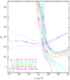 |
Fig. 8. Example of constraints on the number densities of hydrogen nuclei, nPDR, and the FUV radiation fields, G0, obtained for PLCK_G045.1+61.1 using the PDR models from Kaufman et al. (1999, 2006). Contours show the CO, [C I] and [C II] luminosity ratios, as labeled in the caption, with solid lines showing the average ratios and dotted lines their 1σ uncertainties. |
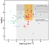 |
Fig. 9. Results of the PDR modeling of the Planck’s dusty GEMS using line luminosity ratios of CO, [C I], and [C II] (red points, see further details in the text), with error bars showing the 1σ uncertainties on the best-fitting values. The average PDR densities, nPDR, correspond to number densities of hydrogen nuclei and the FUV radiation fields, G0, are given in Habing units (1.6 × 10⁻³ erg cm−2 s−1). The sources without [C I](1–0) detection are plotted in light red. We compare with other SMGs in the literature (blue points, Cox et al. 2011; Danielson et al. 2011; Valtchanov et al. 2011; Alaghband-Zadeh et al. 2013; Huynh et al. 2014; Rawle et al. 2014; Bothwell et al. 2017), with the regimes of local normal star-forming galaxies (green points, Malhotra et al. 2001), and local ULIRGs (orange region, Davies et al. 2003), and with the average position of nearby galaxy populations and Galactic regions inferred in Stacey et al. (1991) using [C II]/CO(1–0) line ratios (hatched regions). The physical conditions in the GEMS closely resemble those of local ULIRGs and starbursts, with very similar densities in the range nPDR = 104–105 cm−3. The PDR models also suggest that some Planck’s dusty GEMS are illuminated by lower FUV radiation fields, more typical of local spiral galaxies and molecular clouds in the Milky Way. |
These results compare well with the values G0 = 102.2–104.5 obtained for z = 1–4 SMGs in Wardlow et al. (2017), by modeling the PDR conditions from stacked spectra of the [O I]63μm and [Si II]34μm fine-structure lines in eight to 37 sources, and measurements of [C II] from the literature. However, this study finds average gas densities of 10–1000 cm−3, about two orders of magnitude lower than for other SMGs. This difference could be partly due to selection biases, systematic uncertainties from the stacking analysis that involves both lensed and unlensed SMGs, or possibly because these fine-structure lines probe different gas regions than CO and C I in these high-redshift environments, leading to complex geometric effects. As noted in Wardlow et al. (2017), the difficulty in correctly assessing the level of [O I]63μm self-absorption might also influence the resulting PDR densities (see also Vasta et al. 2010).
In Fig. 9, we compare the best-fitting values of nPDR and G0 with the regimes covered by local populations of star-forming galaxies. The PDRs in the Planck’s dusty GEMS are denser than those in the representative sample of normal star-forming galaxies with [C II] and [O I] detections from Malhotra et al. (2001). The PDR densities in the GEMS correspond very well to those obtained in the nuclei of local ULIRGs by modeling the ratios of near-infrared molecular hydrogen lines (Davies et al. 2003), and are slightly lower than those within the dense cores of Galactic giant molecular clouds (e.g., Bergin et al. 1996). In addition, we show the FUV radiation fields derived from [C II]/CO(1–0) line luminosity ratios in Stacey et al. (1991) for local starbursts and non-starburst spiral galaxies, starburst cores, and giant molecular clouds and denser OB star-forming regions in the Milky Way. For most of the GEMS, the G0 values closely resemble those measured in nearby ULIRGs and bluer starbursts. The models of PLCK_G045.1+61.1, PLCK_G080.2+49.8, PLCK_G145.2+50.9, and PLCK_G200.6+46.1 nonetheless indicate that the PDRs in these GEMS are illuminated by less intense radiation fields, more typical to the regimes of local spiral galaxies and Galactic molecular clouds (Stacey et al. 1991), but still 2–3 orders of magnitude stronger than the average value in the local Galactic ISM. Moreover, the conditions in the GEMS imply average PDR surface temperatures of 100–800 K.
The results of this PDR analysis generally suggest that the most intense dust-obscured starbursts at z = 2–4 have ISM properties akin to various low-redshift environments, ranging from the central regions of ULIRGs triggered by major mergers and of bluer starburst galaxies, to normal star-forming galaxies and the dense Galactic star-forming clouds illuminated by young stars. High spatial resolution interferometric observations of multiple gas tracers combined with high magnifications are required to resolve individual giant molecular clouds in gravitationally lensed high-redshift dusty starbursts and further investigate the conditions within individual PDRs, as well as constraining their sizes and finding their local counterparts.
6. Discussion
6.1. Gas density estimates
Our density estimates from the LVG and PDR models presented in Tables 3 and 4 differ by about one order of magnitude, and average PDR densities, nPDR = nH + 2 × nH2, are higher than nH2 measured on the integrated CO SLEDs (akin to results of Danielson et al. 2011, for the Cosmic Eyelash). For half of the GEMS4, the molecular hydrogen densities derived with the relation nH2 ≃ nPDR/2 are significantly higher than those obtained from the best-fitting LVG models, either with one or two excitation components. Our temperature estimates do not exhibit such discrepancy, since the PDR surface temperatures of Table 4 are within 1σ of the kinetic temperatures from the LVG analysis.
The difference must therefore lie in the different assumptions inherent to each density estimate. Firstly, LVG model parameters are recovered with typical uncertainties of 0.5 dex and up to 1 dex, as also shown by Tunnard & Greve (2016), with possibly some additional dependence on the choice of the relation between escape probability and optical depth (van der Tak et al. 2007). Secondly, the outputs of PDR models vary for different configurations of the incident radiation field, cloud geometries and density distributions throughout the PDR (Spaans 1996). Our assumption of a unique, homogeneous PDR with a single external FUV source is certainly simplistic and, interestingly, Kaufman et al. (1999) and Wolfire et al. (1990) note that applying these models to entire galaxies rather than individual PDRs leads to density and G0 estimates biased to high values. Nonetheless, although lacking detailed constraints on the internal structure of gas clouds only allows us to derive rough estimates of the physical ISM conditions in the GEMS, averaging over the sample provides valuable comparisons between low and high-redshift populations, which is the main scope of this analysis.
It is also possible that additional heating mechanisms contribute. For example mechanical heating can harden the UV radiation fields even in photon-dominated regions (e.g., Kazandjian et al. 2012), and would predominantly boost the high-J lines, thereby mimicking elevated gas densities (Kazandjian et al. 2015). This is an interesting possibility for the GEMS given their intense star formation and broad line widths, perhaps a sign of strong turbulence (as found for the Ruby, Cañameras et al. 2017a). However, a detailed analysis is beyond the scope of this paper.
6.2. Estimates of the PDR sizes
We followed Danielson et al. (2011) in deriving rough estimates of the azimuthally-averaged sizes of the GEMS, using the total CO-inferred masses of molecular gas directly related to the on-going star formation from Sect. 5.2 and the best-fitting molecular gas densities from the PDR analysis (nH2 ≃ nPDR/2, assuming negligible atomic hydrogen densities). This calculation assumes that all the molecular gas is uniformly distributed over the galaxies, which is known to be a strong assumption, since the intense dust-obscured star formation in the GEMS and other high-redshift SMGs has proven to be irregular, either due to mergers (e.g., Engel et al. 2010), or clumpy gas distributions over extended disks (e.g., Swinbank et al. 2011).
Spheres of mass equal to the measured MCO(H2) would have typical radii, R, ranging between 130 and 340 pc to match the best-fitting gas densities. Alternatively, using a 100-pc thick disk model we obtain radii between 150 and 720 pc. For the Ruby, where we have direct, resolved constraints on scales of 100 pc from ALMA dust continuum and CO(4–3) interferometry (Cañameras et al. 2017a), we obtained radii of 130 pc and 165 pc for the sphere and disk models, respectively, slightly larger than the intrinsic size of individual clumps, but smaller than the total starburst size. Since these simple estimates result from the PDR densities, which are constrained by mid-J CO lines and from the gas masses extrapolated from the LVG excitation analysis, they correspond to the extent of the gas reservoirs fueling star formation and suggest that this gas phase is more compact than the overall dust continuum emission (taken as the system size, see Table 1).
Alternatively, the relation  from Wolfire et al. (1990) allows us to convert the incident FUV radiation field for PDRs randomly distributed within a galaxy of total FIR luminosity, LFIR, to the total size of the area covered by the PDRs, RPDR. We assumed that RPDR is equal to the total size of the gas reservoirs, including the extended and low density component suggested by the CO SLED for some sources, and we followed Stacey et al. (2010) in using this relation, together with measurements available in the literature for the local starburst M 82, to infer the sizes of the GEMS (see also Gullberg et al. 2015; Wardlow et al. 2017). We obtained the source radii listed in Table 4, which range between 0.8 and 5.8 kpc, akin to the typical Gaussian half-width at half maximum sizes of the molecular gas reservoirs in high-redshift compact starbursts and SMGs of about 0.5–5 kpc (e.g., Ivison et al. 2011; Bussmann et al. 2013; Ikarashi et al. 2015). Despite the large uncertainties inherent to this scaling relation, the resulting PDR sizes are remarkably similar to the intrinsic dimensions of PLCK_G165.7+67.0 and PLCK_G244.8+54.9 in Table 1, the two GEMS with high-resolution SMA or ALMA interferometry, providing robust measurements of the delensed dust sizes. This suggests that the overall gas reservoirs extend over kpc scales, comparable to those covered by the cold dust continuum and about ten times larger than the intense star-forming clumps identified in some of the sources.
6.3. Constraints on additional heating mechanisms
Studies simulating the chemical composition of photon and X-ray dominated regions (XDR) as a function of their physical properties have claimed that luminosity ratios of CO lines can be used to distinguish effectively the gas clouds heated by the FUV radiation field from star formation (PDR) from those primarily irradiated by X-ray emission from an AGN (XDR). We can therefore use our CO line survey to search for signatures of AGN heating on the molecular gas reservoirs in the GEMS. We used the grid of PDR and XDR models from Meijerink & Spaans (2005) and Meijerink et al. (2007), which suggest that CO line ratios, in particular those between high-J transitions (Jup ≥ 10) and CO(1–0), are significantly higher in XDRs. The reason is that, for a given energy injection from external radiation fields, CO emission will arise from smaller physical scales and warmer environments in XDRs. We compared the observed line ratios with those simulated in Meijerink et al. (2007) for the high density model, the most representative for spatially-integrated gas conditions in SMGs, which also covers the PDR properties in the GEMS. For n = 104–106.5 cm−3 and G0 = 102–105 Habing fields, the high-J CO versus CO(1–0) line ratios increase with the external radiation fields and are significantly higher in XDRs.
The ratios measured in the GEMS are systematically lower than those predicted by the model over this density range. This also holds when using only the highest and lowest-J CO lines detected with EMIR. For instance, we find LCO(10 − 9)/LCO(1 − 0) = 25 ± 11 for PLCK_G092.5+42.9, while Meijerink et al. (2007) obtain a lower limit on this luminosity ratio of approximately 400 in XDRs. Although atomic carbon diagnostics suggest that PLCK_G138.6+62.0 falls in the regime covered both by PDRs and XDRs (N18), we find LCO(7 − 6)/LCO(1 − 0) and LCO(7 − 6)/LCO(3 − 2) to be lower than those in the grid of XDR models by a factor of about 3–4. Consequently, there is no evidence that gas heating in the GEMS can be attributed to incident X-ray radiation fields from a central AGN above the lower value of 1.6 erg s−1 cm−2 considered in the models. This is consistent with the minor AGN contribution to the overall dust heating obtained in C15 and our choice of describing the integrated line emission with PDR models in Sect. 5.3. Other ratios involving dense gas tracers (e.g., HCN/HCO+) would further constrain the upper limits on the incident X-ray fields.
7. Summary
In this paper, we have presented an analysis of the physical properties of highly-excited molecular gas reservoirs in the Planck’s dusty GEMS, a small set of the brightest strongly lensed high-redshift dusty star-forming galaxies on the extragalactic sky identified with the Planck and Herschel satellites, using an extensive CO emission-line survey with EMIR on the IRAM 30-m telescope. We detected 45 CO rotational lines from Jup = 3 to Jup = 11 in the 11 submillimeter sources, ranging between z = 2.2 and z = 3.6, with velocity-integrated fluxes up to 37 μ−1 Jy km s−1. The line profiles are broad, with FWHM = 200–750 km s−1, and they are well-fitted with single Gaussians for seven sources while the remaining four show evidence for double velocity components over multiple Jup values.
Firstly, using the well-sampled CO spectral-line energy distributions from mid- to high-J with up to eight transitions per source and published CO(1–0) observations, we performed a detailed analysis of the CO gas excitation to shed light on the conditions of the ISM within these intense dusty starbursts. The peak of the CO ladder falls between Jup = 4 and Jup = 7 for nine out of 11 sources. Moreover, the two brightest GEMS, PLCK_G092.5+42.9 and PLCK_G244.8+54.9, exhibit double peaks with a highly-excited, warm gas component reaching a maximum at Jup > 7. These results are globally consistent with the broad range of gas excitations found amongst the population of lensed and unlensed SMGs, and with the inner regions of low-redshift starburst galaxies such as Arp 220 and M 82.
Our detailed lensing models from resolved dust continuum and mid-J CO line interferometry, and the EMIR CO line profiles, suggest that differential lensing does not play a major role in this analysis. In the worst case, this effect might induce uncertainties comparable to those from other assumptions (e.g., on the spatial configuration of the gas reservoirs), and we ignored its impact on the CO SLEDs and resulting gas properties.
Secondly, we characterized the gas excitation from radiative transfer LVG models of the spatially-integrated CO flux ratios, following a similar approach as in Yang et al. (2017). For a single excitation component, we obtained average densities nH2 = 102.6 − 104.1 cm−3, kinetic temperatures Tk = 30–1000 K and column densities of CO normalized per unit velocity gradient NCO/dv = 1016–1017.5 cm−2 km−1 s for the bulk of the molecular gas reservoirs in the Planck’s dusty GEMS. For five sources, our well-sampled CO ladders highlight two gas phases with different properties and we reproduced our analysis using two excitation components. We found elevated densities, nH2 = 103.0–104.5 cm−3, and temperatures of about 70–320 K for the warm gas reservoirs with high excitation. The properties of the cooler and more extended low-excitation component in PLCK_G092.5+42.9 and PLCK_G244.8+54.9 are similar to average conditions in local ULIRGs but, for PLCK_G113.7+61.0 and PLCK_G138.6+62.0 this component is diffuse, with nH2 = 102.4–102.8 cm−3. This suggests that some high-redshift dusty starbursts contain a cool, low-density gas phase, comparable to that over the Galactic disk. Moreover, deblending individual kinematic components in three sources provides hints of varying CO excitations in two of them.
Thirdly, the intrinsic molecular gas masses derived from the best-fitting excitation models of the Jup > 3 CO ladder and αCO = 0.8 M⊙ (K km s−1 pc2)−1 range from 0.6 to 12 × 1010 M⊙, implying an average gas-to-dust ratio of 150. These models predict lower CO(1–0) fluxes than those measured with the GBT for five sources. We interprete these low rJ ≥ 3, 1 ratios as additional evidence for a diffuse gas phase, rather than differential magnification, and find that 20–50% of the total gas masses are embedded within these reservoirs, provided that the relative IRAM/GBT flux calibrations are robust.
Lastly, the CO line-luminosity ratios are consistent with those predicted by models of photon-dominated regions and disfavor scenarios in which the gas clouds are irradiated by intense X-ray fields from AGNs. We combined these transitions with single-dish [C I] line detections presented in a companion paper as well as other [C II] measurements from the literature to derive PDR models (Kaufman et al. 1999) and infer the global ISM conditions of the Planck’s dusty GEMS. Our EMIR line detections provide robust constraints on the PDR gas densities, nPDR = 104–105 cm−3, higher than in local normal star-forming galaxies. This results in molecular hydrogen densities greater than those obtained with the LVG models, possibly due to geometric effects or contributions from mechanical heating. The FUV radiation fields from newly formed stellar populations are intense, from 102 to 104 times that of the Milky Way disk, although we caution that for some GEMS, G0 depends strongly on our choice of the [C II] luminosity. These spatially-averaged conditions are consistent with other high-redshift SMGs and cover various low-redshift environments, ranging from the cores of ULIRGs, to bluer starbursts and dense Galactic molecular clouds. PDR radii are of order of 1–6 kpc, showing that the overall gas reservoirs and delensed dust continuum sizes are comparable, and nearly one order of magnitude larger than for individual star-forming clumps.
Our study demonstrates the need to perform extensive line surveys to fully characterize the CO excitation and number of ISM phases in high-redshift SMGs, and that spatially-averaged properties of this population cover a range of low-redshift environments. In the future, combining high spatial resolution interferometry of multiple gas tracers and strong gravitational magnifications will be an ideal way to probe the range of physical conditions within individual giant molecular clouds in high-redshift dusty starbursts, and constrain the local mechanisms setting the star-formation efficiency.
In particular for PLCK_G138.6+62.0, PLCK_G165.7+67.0, PLCK_G200.6+46.1, PLCK_G231.3+72.2 and PLCK_G244.8+54.9.
Acknowledgments
RC would like to thank Raphael Gavazzi for useful discussions. The authors would like to thank the anonymous referee, whose comments were helpful in improving the paper, and the telescope staff at the IRAM 30-m telescope for their excellent support during observations. We are also very grateful to the former director of IRAM, P. Cox, for his generous attribution of Director’s Discretionary Time early on during the program, and to Daniel Dicken for sharing telescope time. This work is based on observations carried out under projects number 082-12, D09-12, 065-13, 094-13, 223-13, 108-14, and 217-14 with the IRAM 30-m telescope. IRAM is supported by INSU/CNRS (France), MPG (Germany) and IGN (Spain). This work was supported by the Programme National Cosmology et Galaxies (PNCG) of CNRS/INSU with INP and IN2P3, co-funded by CEA and CNES. RC was supported by DFF – 4090-00079. ML acknowledges CNRS and CNES for support. CY was supported by an ESO Fellowship.
References
- Abel, N. P. 2006, MNRAS, 368, 1949 [NASA ADS] [CrossRef] [Google Scholar]
- Alaghband-Zadeh, S., Chapman, S. C., Swinbank, A. M., et al. 2013, MNRAS, 435, 1493 [Google Scholar]
- Aravena, M., Spilker, J. S., Bethermin, M., et al. 2016, MNRAS, 457, 4406 [NASA ADS] [CrossRef] [Google Scholar]
- Bergin, E. A., Snell, R. L., & Goldsmith, P. F. 1996, ApJ, 460, 343 [NASA ADS] [CrossRef] [Google Scholar]
- Blain, A. W. 1999, MNRAS, 304, 669 [NASA ADS] [CrossRef] [Google Scholar]
- Bolatto, A. D., Wolfire, M., & Leroy, A. K. 2013, ARA&A, 51, 207 [Google Scholar]
- Bothwell, M. S., Smail, I., Chapman, S. C., et al. 2013, MNRAS, 429, 3047 [NASA ADS] [CrossRef] [Google Scholar]
- Bothwell, M. S., Aguirre, J. E., Aravena, M., et al. 2017, MNRAS, 466, 2825 [Google Scholar]
- Bradford, C. M., Nikola, T., Stacey, G. J., et al. 2003, ApJ, 586, 891 [NASA ADS] [CrossRef] [Google Scholar]
- Bradford, C. M., Bolatto, A. D., Maloney, P. R., et al. 2011, ApJ, 741, L37 [NASA ADS] [CrossRef] [Google Scholar]
- Braine, J., & Combes, F. 1992, A&A, 264, 433 [NASA ADS] [Google Scholar]
- Bussmann, R. S., Pérez-Fournon, I., Amber, S., et al. 2013, ApJ, 779, 25 [NASA ADS] [CrossRef] [Google Scholar]
- Cañameras, R., Nesvadba, N. P. H., Guery, D., et al. 2015, A&A, 581, A105 [NASA ADS] [CrossRef] [EDP Sciences] [Google Scholar]
- Cañameras, R., Nesvadba, N., Kneissl, R., et al. 2017a, A&A, 604, A117 [NASA ADS] [CrossRef] [EDP Sciences] [Google Scholar]
- Cañameras, R., Nesvadba, N. P. H., Kneissl, R., et al. 2017b, A&A, 600, L3 [NASA ADS] [CrossRef] [EDP Sciences] [Google Scholar]
- Cañameras, R., Nesvadba, N. P. H., & Limousin, M. 2018, A&A, 620, A60 [NASA ADS] [CrossRef] [EDP Sciences] [Google Scholar]
- Carilli, C. L., & Walter, F. 2013, ARA&A, 51, 105 [NASA ADS] [CrossRef] [EDP Sciences] [Google Scholar]
- Carter, M., Lazareff, B., Maier, D., et al. 2012, A&A, 538, A89 [NASA ADS] [CrossRef] [EDP Sciences] [Google Scholar]
- Casey, C. M., Narayanan, D., & Cooray, A. 2014, Phys. Rep., 541, 45 [NASA ADS] [CrossRef] [Google Scholar]
- Cox, P., Krips, M., Neri, R., et al. 2011, ApJ, 740, 63 [NASA ADS] [CrossRef] [Google Scholar]
- da Cunha, E., Groves, B., Walter, F., et al. 2013, ApJ, 766, 13 [Google Scholar]
- Daddi, E., Bournaud, F., Walter, F., et al. 2010, ApJ, 713, 686 [NASA ADS] [CrossRef] [Google Scholar]
- Daddi, E., Dannerbauer, H., Liu, D., et al. 2015, A&A, 577, A46 [NASA ADS] [CrossRef] [EDP Sciences] [Google Scholar]
- Danielson, A. L. R., Swinbank, A. M., Smail, I., et al. 2011, MNRAS, 410, 1687 [NASA ADS] [Google Scholar]
- Dannerbauer, H., Daddi, E., Riechers, D. A., et al. 2009, ApJ, 698, L178 [NASA ADS] [CrossRef] [Google Scholar]
- Davies, R. I., Sternberg, A., Lehnert, M., & Tacconi-Garman, L. E. 2003, ApJ, 597, 907 [NASA ADS] [CrossRef] [Google Scholar]
- Decarli, R., Walter, F., Carilli, C., et al. 2014, ApJ, 782, L17 [NASA ADS] [CrossRef] [Google Scholar]
- Dunlop, J. S., McLure, R. J., Biggs, A. D., et al. 2017, MNRAS, 466, 861 [NASA ADS] [CrossRef] [Google Scholar]
- Engel, H., Tacconi, L. J., Davies, R. I., et al. 2010, ApJ, 724, 233 [NASA ADS] [CrossRef] [Google Scholar]
- Fixsen, D. J., Bennett, C. L., & Mather, J. C. 1999, ApJ, 526, 207 [NASA ADS] [CrossRef] [Google Scholar]
- Frye, B. L., Pascale, M., Zitrin, A., et al. 2018, ApJ, submitted [arXiv:1805.04790] [Google Scholar]
- Genzel, R., Tacconi, L. J., Lutz, D., et al. 2015, ApJ, 800, 20 [NASA ADS] [CrossRef] [Google Scholar]
- Gerin, M., Ruaud, M., Goicoechea, J. R., et al. 2015, A&A, 573, A30 [NASA ADS] [CrossRef] [EDP Sciences] [Google Scholar]
- Goldsmith, P. F., Langer, W. D., Pineda, J. L., & Velusamy, T. 2012, ApJS, 203, 13 [Google Scholar]
- Greve, A., Panis, J.-F., & Thum, C. 1996, A&AS, 115, 379 [NASA ADS] [Google Scholar]
- Greve, T. R., Leonidaki, I., Xilouris, E. M., et al. 2014, ApJ, 794, 142 [NASA ADS] [CrossRef] [Google Scholar]
- Gullberg, B., De Breuck, C., Vieira, J. D., et al. 2015, MNRAS, 449, 2883 [NASA ADS] [CrossRef] [Google Scholar]
- Hainline, L. J., Blain, A. W., Greve, T. R., et al. 2006, ApJ, 650, 614 [NASA ADS] [CrossRef] [Google Scholar]
- Harrington, K. C., Yun, M. S., Cybulski, R., et al. 2016, MNRAS, 458, 4383 [NASA ADS] [CrossRef] [Google Scholar]
- Harrington, K. C., Yun, M. S., Magnelli, B., et al. 2018, MNRAS, 474, 3866 [NASA ADS] [CrossRef] [Google Scholar]
- Harris, A. I., Baker, A. J., Zonak, S. G., et al. 2010, ApJ, 723, 1139 [NASA ADS] [CrossRef] [Google Scholar]
- Harris, A. I., Baker, A. J., Frayer, D. T., et al. 2012, ApJ, 752, 152 [NASA ADS] [CrossRef] [Google Scholar]
- Hauser, M. G., & Dwek, E. 2001, ARA&A, 39, 249 [NASA ADS] [CrossRef] [Google Scholar]
- Hezaveh, Y. D., Marrone, D. P., & Holder, G. P. 2012, ApJ, 761, 20 [NASA ADS] [CrossRef] [Google Scholar]
- Hodge, J. A., Carilli, C. L., Walter, F., Daddi, E., & Riechers, D. 2013, ApJ, 776, 22 [NASA ADS] [CrossRef] [Google Scholar]
- Hollenbach, D. J., & Tielens, A. G. G. M. 1997, ARA&A, 35, 179 [NASA ADS] [CrossRef] [Google Scholar]
- Huynh, M. T., Kimball, A. E., Norris, R. P., et al. 2014, MNRAS, 443, L54 [NASA ADS] [CrossRef] [Google Scholar]
- Ikarashi, S., Ivison, R. J., Caputi, K. I., et al. 2015, ApJ, 810, 133 [NASA ADS] [CrossRef] [Google Scholar]
- Ivison, R. J., Swinbank, A. M., Swinyard, B., et al. 2010, A&A, 518, L35 [NASA ADS] [CrossRef] [EDP Sciences] [Google Scholar]
- Ivison, R. J., Papadopoulos, P. P., Smail, I., et al. 2011, MNRAS, 412, 1913 [NASA ADS] [CrossRef] [Google Scholar]
- Jiao, Q., Zhao, Y., Zhu, M., et al. 2017, ApJ, 840, L18 [NASA ADS] [CrossRef] [Google Scholar]
- Jullo, E., Kneib, J.-P., Limousin, M., et al. 2007, New J. Phys., 9, 447 [Google Scholar]
- Kamenetzky, J., Rangwala, N., Glenn, J., Maloney, P. R., & Conley, A. 2016, ApJ, 829, 93 [NASA ADS] [CrossRef] [Google Scholar]
- Kamenetzky, J., Privon, G. C., & Narayanan, D. 2018, ApJ, 859, 9 [NASA ADS] [CrossRef] [Google Scholar]
- Kaufman, M. J., Wolfire, M. G., Hollenbach, D. J., & Luhman, M. L. 1999, ApJ, 527, 795 [NASA ADS] [CrossRef] [Google Scholar]
- Kaufman, M. J., Wolfire, M. G., & Hollenbach, D. J. 2006, ApJ, 644, 283 [NASA ADS] [CrossRef] [Google Scholar]
- Kazandjian, M. V., Meijerink, R., Pelupessy, I., Israel, F. P., & Spaans, M. 2012, A&A, 542, A65 [NASA ADS] [CrossRef] [EDP Sciences] [Google Scholar]
- Kazandjian, M. V., Meijerink, R., Pelupessy, I., Israel, F. P., & Spaans, M. 2015, A&A, 574, A127 [NASA ADS] [CrossRef] [EDP Sciences] [Google Scholar]
- Le Petit, F., Nehmé, C., Le Bourlot, J., & Roueff, E. 2006, ApJS, 164, 506 [NASA ADS] [CrossRef] [EDP Sciences] [Google Scholar]
- Lehnert, M. D., Nesvadba, N. P. H., Le Tiran, L., et al. 2009, ApJ, 699, 1660 [NASA ADS] [CrossRef] [Google Scholar]
- Liu, D., Gao, Y., Isaak, K., et al. 2015, ApJ, 810, L14 [NASA ADS] [CrossRef] [Google Scholar]
- Lu, N., Zhao, Y., Díaz-Santos, T., et al. 2017, ApJS, 230, 1 [NASA ADS] [CrossRef] [Google Scholar]
- Madden, S. C., Geis, N., Genzel, R., et al. 1993, ApJ, 407, 579 [NASA ADS] [CrossRef] [Google Scholar]
- Magnelli, B., Popesso, P., Berta, S., et al. 2013, A&A, 553, A132 [NASA ADS] [CrossRef] [EDP Sciences] [Google Scholar]
- Malhotra, S., Kaufman, M. J., Hollenbach, D., et al. 2001, ApJ, 561, 766 [Google Scholar]
- Meijerink, R., & Spaans, M. 2005, A&A, 436, 397 [NASA ADS] [CrossRef] [EDP Sciences] [Google Scholar]
- Meijerink, R., Spaans, M., & Israel, F. P. 2007, A&A, 461, 793 [NASA ADS] [CrossRef] [EDP Sciences] [Google Scholar]
- Meijerink, R., Spaans, M., Loenen, A. F., & van der Werf, P. P. 2011, A&A, 525, A119 [NASA ADS] [CrossRef] [EDP Sciences] [Google Scholar]
- Narayanan, D., & Krumholz, M. R. 2014, MNRAS, 442, 1411 [NASA ADS] [CrossRef] [Google Scholar]
- Negrello, M., Perrotta, F., González-Nuevo, J., et al. 2007, MNRAS, 377, 1557 [NASA ADS] [CrossRef] [Google Scholar]
- Negrello, M., Hopwood, R., De Zotti, G., et al. 2010, Science, 330, 800 [NASA ADS] [CrossRef] [Google Scholar]
- Nesvadba, N., Kneissl, R., Cañameras, R., et al. 2016, A&A, 593, L2 [NASA ADS] [CrossRef] [EDP Sciences] [Google Scholar]
- Nesvadba, N. P. H., Cañameras, R., & Kneissl, R. 2018, A&A, submitted [Google Scholar]
- Papadopoulos, P. P. 2010, ApJ, 720, 226 [NASA ADS] [CrossRef] [Google Scholar]
- Papadopoulos, P. P., Thi, W.-F., & Viti, S. 2004, MNRAS, 351, 147 [NASA ADS] [CrossRef] [Google Scholar]
- Pearson, C., Rigopoulou, D., Hurley, P., et al. 2016, ApJS, 227, 9 [NASA ADS] [CrossRef] [Google Scholar]
- Planck Collaboration Int. XXVII. 2015, A&A, 582, A30 [NASA ADS] [CrossRef] [EDP Sciences] [Google Scholar]
- Planck Collaboration XIII. 2016, A&A, 594, A13 [NASA ADS] [CrossRef] [EDP Sciences] [Google Scholar]
- Pound, M. W., & Wolfire, M. G. 2008, in Astronomical Data Analysis Software and Systems XVII, eds. R. W. Argyle, P. S. Bunclark, & J. R. Lewis, ASP Conf. Ser., 394, 654 [NASA ADS] [Google Scholar]
- Rangwala, N., Maloney, P. R., Glenn, J., et al. 2011, ApJ, 743, 94 [NASA ADS] [CrossRef] [Google Scholar]
- Rawle, T. D., Egami, E., Bussmann, R. S., et al. 2014, ApJ, 783, 59 [NASA ADS] [CrossRef] [Google Scholar]
- Riechers, D. A., Bradford, C. M., Clements, D. L., et al. 2013, Nature, 496, 329 [Google Scholar]
- Rigopoulou, D., Hopwood, R., Magdis, G. E., et al. 2014, ApJ, 781, L15 [NASA ADS] [CrossRef] [Google Scholar]
- Rosenberg, M. J. F., van der Werf, P. P., Aalto, S., et al. 2015, ApJ, 801, 72 [NASA ADS] [CrossRef] [Google Scholar]
- Rowlands, K., Wild, V., Nesvadba, N., et al. 2015, MNRAS, 448, 258 [NASA ADS] [CrossRef] [Google Scholar]
- Rybak, M., Vegetti, S., McKean, J. P., Andreani, P., & White, S. D. M. 2015, MNRAS, 453, L26 [NASA ADS] [CrossRef] [Google Scholar]
- Scoville, N., Murchikova, L., Walter, F., et al. 2017, ApJ, 836, 66 [NASA ADS] [CrossRef] [Google Scholar]
- Serjeant, S. 2012, MNRAS, 424, 2429 [NASA ADS] [CrossRef] [Google Scholar]
- Sharon, C. E., Riechers, D. A., Hodge, J., et al. 2016, ApJ, 827, 18 [Google Scholar]
- Solomon, P. M., & Vanden Bout, P. A. 2005, ARA&A, 43, 677 [NASA ADS] [CrossRef] [Google Scholar]
- Solomon, P. M., Downes, D., & Radford, S. J. E. 1992, ApJ, 398, L29 [NASA ADS] [CrossRef] [Google Scholar]
- Solomon, P. M., Downes, D., Radford, S. J. E., & Barrett, J. W. 1997, ApJ, 478, 144 [NASA ADS] [CrossRef] [Google Scholar]
- Spaans, M. 1996, A&A, 307, 271 [NASA ADS] [Google Scholar]
- Spilker, J. S., Aravena, M., Marrone, D. P., et al. 2015, ApJ, 811, 124 [NASA ADS] [CrossRef] [Google Scholar]
- Stacey, G. J., Geis, N., Genzel, R., et al. 1991, ApJ, 373, 423 [NASA ADS] [CrossRef] [Google Scholar]
- Stacey, G. J., Hailey-Dunsheath, S., Ferkinhoff, C., et al. 2010, ApJ, 724, 957 [NASA ADS] [CrossRef] [Google Scholar]
- Swinbank, A. M., Smail, I., Longmore, S., et al. 2010, Nature, 464, 733 [Google Scholar]
- Swinbank, A. M., Papadopoulos, P. P., Cox, P., et al. 2011, ApJ, 742, 11 [NASA ADS] [CrossRef] [Google Scholar]
- Tacconi, L. J., Genzel, R., Smail, I., et al. 2008, ApJ, 680, 246 [NASA ADS] [CrossRef] [PubMed] [Google Scholar]
- Tacconi, L. J., Genzel, R., Neri, R., et al. 2010, Nature, 463, 781 [Google Scholar]
- Thomson, A. P., Ivison, R. J., Owen, F. N., et al. 2015, MNRAS, 448, 1874 [NASA ADS] [CrossRef] [Google Scholar]
- Tunnard, R., & Greve, T. R. 2016, ApJ, 819, 161 [NASA ADS] [CrossRef] [Google Scholar]
- Valtchanov, I., Virdee, J., Ivison, R. J., et al. 2011, MNRAS, 415, 3473 [NASA ADS] [CrossRef] [Google Scholar]
- van der Tak, F. F. S., Black, J. H., Schöier, F. L., Jansen, D. J., & van Dishoeck, E. F. 2007, A&A, 468, 627 [NASA ADS] [CrossRef] [EDP Sciences] [Google Scholar]
- Vasta, M., Barlow, M. J., Viti, S., Yates, J. A., & Bell, T. A. 2010, MNRAS, 404, 1910 [NASA ADS] [Google Scholar]
- Vieira, J. D., Marrone, D. P., Chapman, S. C., et al. 2013, Nature, 495, 344 [NASA ADS] [CrossRef] [Google Scholar]
- Wagg, J., Wilner, D. J., Neri, R., Downes, D., & Wiklind, T. 2006, ApJ, 651, 46 [NASA ADS] [CrossRef] [Google Scholar]
- Wardlow, J. L., Cooray, A., De Bernardis, F., et al. 2013, ApJ, 762, 59 [NASA ADS] [CrossRef] [Google Scholar]
- Wardlow, J. L., Cooray, A., Osage, W., et al. 2017, ApJ, 837, 12 [NASA ADS] [CrossRef] [Google Scholar]
- Weiß, A., Walter, F., & Scoville, N. Z. 2005, A&A, 438, 533 [NASA ADS] [CrossRef] [EDP Sciences] [Google Scholar]
- Weiß, A., Downes, D., Neri, R., et al. 2007, A&A, 467, 955 [NASA ADS] [CrossRef] [EDP Sciences] [Google Scholar]
- Wiedner, M. C., Wilson, C. D., Harrison, A., et al. 2002, ApJ, 581, 229 [NASA ADS] [CrossRef] [Google Scholar]
- Wolfire, M. G., Tielens, A. G. G. M., & Hollenbach, D. 1990, ApJ, 358, 116 [NASA ADS] [CrossRef] [Google Scholar]
- Yang, C., Omont, A., Beelen, A., et al. 2017, A&A, 608, A144 [NASA ADS] [CrossRef] [EDP Sciences] [Google Scholar]
- Young, J. S., & Scoville, N. Z. 1991, ARA&A, 29, 581 [NASA ADS] [CrossRef] [Google Scholar]
- Zhang, Z.-Y., Papadopoulos, P. P., Ivison, R. J., et al. 2016, R. Soc. Open Sci., 3, 160025 [Google Scholar]
Appendix A: Profiles and measured properties of the CO rotational lines
Tables A.1 and A.2 present the observation log with EMIR and the properties of each CO emission line, respectively. The spatially-integrated and binned spectra of all observed CO lines are shown in Figs. A.1–A.3, after subtracting the continuum baselines fitted on line-free spectral channels. All spectra from a given source were fitted consistently with a single or two Gaussian components.
Observation log with EMIR on the IRAM 30-m telescope.
Properties of the CO emission lines obtained by fitting the continuum-subtracted spectra using a single or two Gaussian components with CLASS.
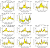 |
Fig. A.1. Continuum-subtracted and binned spectra of PLCK_G045.1+61.1 (top two rows), PLCK_G080.2+49.8 (third row), and PLCK_G102.1+53.6 (bottom row), fitted with one or two Gaussian components. See further details in Fig. 1 caption. |
 |
Fig. A.2. Continuum-subtracted and binned spectra of PLCK_G092.5+42.9 (top two rows), PLCK_G113.7+61.0 (third and fourth rows), and PLCK_G138.6+62.0 (bottom two rows), fitted with one or two Gaussian components. See further details in Fig. 1 caption. |
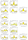 |
Fig. A.3. Continuum-subtracted and binned spectra of PLCK_G145.2+50.9 (first row), PLCK_G165.7+67.0 (second and third rows), PLCK_G200.6+46.1 (fourth and fifth rows), and PLCK_G231.3+72.2 (bottom row), fitted with one or two Gaussian components. See further details in Fig. 1 caption. |
Appendix B: Results of the RADEX LVG modeling
We show the CO SLEDs resulting from our analysis of the gas excitation, using the MCMC implementation of the LVG models from RADEX (van der Tak et al. 2007; Yang et al. 2017). Figure B.1 presents the single and two-component CO excitation models of the four Planck’s dusty GEMS for which we obtain evidence of two distinct gas phases with different properties. Figure B.2 shows the remaining six sources that are conveniently fitted with a single component. The SLEDs plotted in Fig. B.3 are the best-fit LVG models for individual kinematic components deblended from the spectra of PLCK_G045.1+61.1, PLCK_G092.5+42.9, and PLCK_G244.8+54.9, using the same number of excitation components as for the spectrally-integrated SLEDs.
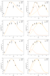 |
Fig. B.1. Best-fit LVG models using RADEX for PLCK_G092.5+42.9 (top), PLCK_G113.7+61.0 (center-top), PLCK_G138.6+62.0 (center-bottom), and PLCK_G165.7+67.0 (bottom), for a single gas excitation component (left) and two components (right). |
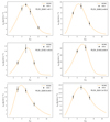 |
Fig. B.2. Single-component models of the gas excitation in the remaining six Planck’s dusty GEMS (see Fig. 6 caption). |
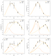 |
Fig. B.3. Best-fit single or double-component LVG models of the gas excitation in the individual blue (left) and red (right) kinematic components of PLCK_G045.1+61.1 (top), PLCK_G092.5+42.9 (center), and PLCK_G244.8+54.9 (bottom). See further details in Fig. 6 caption. |
All Tables
Properties of the Planck’s dusty GEMS that were part of our CO emission-line survey with EMIR.
Estimates of the CO-to-H2 conversion factors, gas masses and gas-to-dust ratios.
Molecular gas properties of the Planck’s dusty GEMS inferred from the MCMC sampling of the LVG model parameter space using RADEX.
Best-fitting values of the average number density of hydrogen nuclei, nPDR, and FUV radiation field, G0, obtained for the Planck’s dusty GEMS using the publicly available implementation of the PDR models from Kaufman et al. (1999, 2006).
Properties of the CO emission lines obtained by fitting the continuum-subtracted spectra using a single or two Gaussian components with CLASS.
All Figures
|
Fig. 1. Single-dish spectra of the CO rotational emission lines in PLCK_G244.8+54.9 observed with EMIR. The continuum-subtracted and binned spectra were fitted with two Gaussian components using the CLASS package of GILDAS, by fixing the peak velocities to those measured on the CO(3–2) spectrum. The best-fit line profiles are plotted as red curves, with the individual spectral components overlaid in gray. Velocity offsets are defined relative to the best spectroscopic redshift z = 3.0054 ± 0.0001 presented in Table 1. The resulting line properties are listed in Table A.2 and EMIR spectra of other Planck’s dusty GEMS are shown in Appendix A. |
| In the text | |
|
Fig. 2. CO spectral-line energy distributions of the Planck’s dusty GEMS. Blue triangles show the velocity-integrated line fluxes uncorrected for gravitational magnification, as measured in this work with EMIR on the IRAM 30-m telescope. All CO(1–0) fluxes are taken from Harrington et al. (2018, black triangles) and CO(3–2) for PLCK_G092.5+42.9 is from Harrington et al. (2016). For PLCK_G045.1+61.1, PLCK_G092.5+42.9, and PLCK_G244.8+54.9, light blue and red triangles show the SLEDs obtained for the blue and red kinematic components, respectively, for the transitions with S/N values sufficiently high to obtain a robust separation of the two components. |
| In the text | |
|
Fig. 3. Relations between LFIR and |
| In the text | |
|
Fig. 4. Observed CO SLEDs normalized by the CO(3–2) line fluxes for the GEMS with CO(3–2) detections (the CO(1–0) fluxes are from Harrington et al. 2018), the local starburst Arp 220 (Wiedner et al. 2002; Rangwala et al. 2011), the central region of M 82 (Weiß et al. 2005) and the Cosmic Eyelash (Danielson et al. 2011). For comparison, we also show the CO SLED spatially-integrated over the inner disk of the Milky Way (dotted line, Fixsen et al. 1999), and the expected trend for optically thick gas in local thermodynamic equilibrium (thick gray line). |
| In the text | |
|
Fig. 5. CO luminosity to gas mass conversion factor, αCO, versus FIR luminosity, for the seven Planck’s dusty GEMS with direct αCO measurements using the molecular gas masses inferred from the [C I](1-0) line fluxes of Nesvadba et al. (2018, red stars). All but one GEMS are consistent with the usual ULIRG value αCO = 0.8 M⊙ (K km s−1 pc2)−1 (lower dashed line). Other points show αCO estimates in the literature, for the strongly lensed SMGs from the SPT survey (blue points), high-redshift unlensed dust-obscured starbursts (green points), QSOs (yellow points) and main sequence galaxies (black squares, Aravena et al. 2016, and references therein). The relative uncertainties on αCO obtained for these high-redshift samples are comparable to those of the GEMS. |
| In the text | |
|
Fig. 6. Top left: observed CO SLED of PLCK_G244.8+54.9, the Ruby (black points), without correcting the velocity-integrated fluxes for gravitational magnification. The orange line shows the best-fit model with RADEX using a single gas excitation component, and illustrates a case where this simple model poorly reproduces the CO ladder for Jup ≳ 6. Top right: best-fit model from RADEX using two gas excitation components (solid orange line). The dot-dashed orange line shows the low excitation component, which is assumed to be cooler and more extended than the high excitation component (dashed yellow line) in the analysis. Bottom: one-dimensional and joint two-dimensional posterior probability distributions of nH2, Tk and NCO/dv, obtained from our MCMC sampling of the RADEX parameter space in the two-component model, for the low (left) and high (right) excitation components. Contours increase in steps of 0.5σ. Yellow and orange solid lines show the maximum posterior probability of each parameter, while dotted lines mark the ±1σ range in the distributions. The resulting parameter values are listed above the corresponding histograms. |
| In the text | |
|
Fig. 7. Results of the gas excitation analysis with RADEX. Red histograms show the median values of the marginal probability distributions of nH2, Tk and NCO/dv obtained by modeling the CO SLEDs with a single excitation component (see Table 3). Blue histograms illustrate how results change when removing the CO(1–0) fluxes from the analysis. |
| In the text | |
|
Fig. 8. Example of constraints on the number densities of hydrogen nuclei, nPDR, and the FUV radiation fields, G0, obtained for PLCK_G045.1+61.1 using the PDR models from Kaufman et al. (1999, 2006). Contours show the CO, [C I] and [C II] luminosity ratios, as labeled in the caption, with solid lines showing the average ratios and dotted lines their 1σ uncertainties. |
| In the text | |
|
Fig. 9. Results of the PDR modeling of the Planck’s dusty GEMS using line luminosity ratios of CO, [C I], and [C II] (red points, see further details in the text), with error bars showing the 1σ uncertainties on the best-fitting values. The average PDR densities, nPDR, correspond to number densities of hydrogen nuclei and the FUV radiation fields, G0, are given in Habing units (1.6 × 10⁻³ erg cm−2 s−1). The sources without [C I](1–0) detection are plotted in light red. We compare with other SMGs in the literature (blue points, Cox et al. 2011; Danielson et al. 2011; Valtchanov et al. 2011; Alaghband-Zadeh et al. 2013; Huynh et al. 2014; Rawle et al. 2014; Bothwell et al. 2017), with the regimes of local normal star-forming galaxies (green points, Malhotra et al. 2001), and local ULIRGs (orange region, Davies et al. 2003), and with the average position of nearby galaxy populations and Galactic regions inferred in Stacey et al. (1991) using [C II]/CO(1–0) line ratios (hatched regions). The physical conditions in the GEMS closely resemble those of local ULIRGs and starbursts, with very similar densities in the range nPDR = 104–105 cm−3. The PDR models also suggest that some Planck’s dusty GEMS are illuminated by lower FUV radiation fields, more typical of local spiral galaxies and molecular clouds in the Milky Way. |
| In the text | |
|
Fig. A.1. Continuum-subtracted and binned spectra of PLCK_G045.1+61.1 (top two rows), PLCK_G080.2+49.8 (third row), and PLCK_G102.1+53.6 (bottom row), fitted with one or two Gaussian components. See further details in Fig. 1 caption. |
| In the text | |
|
Fig. A.2. Continuum-subtracted and binned spectra of PLCK_G092.5+42.9 (top two rows), PLCK_G113.7+61.0 (third and fourth rows), and PLCK_G138.6+62.0 (bottom two rows), fitted with one or two Gaussian components. See further details in Fig. 1 caption. |
| In the text | |
|
Fig. A.3. Continuum-subtracted and binned spectra of PLCK_G145.2+50.9 (first row), PLCK_G165.7+67.0 (second and third rows), PLCK_G200.6+46.1 (fourth and fifth rows), and PLCK_G231.3+72.2 (bottom row), fitted with one or two Gaussian components. See further details in Fig. 1 caption. |
| In the text | |
|
Fig. B.1. Best-fit LVG models using RADEX for PLCK_G092.5+42.9 (top), PLCK_G113.7+61.0 (center-top), PLCK_G138.6+62.0 (center-bottom), and PLCK_G165.7+67.0 (bottom), for a single gas excitation component (left) and two components (right). |
| In the text | |
|
Fig. B.2. Single-component models of the gas excitation in the remaining six Planck’s dusty GEMS (see Fig. 6 caption). |
| In the text | |
|
Fig. B.3. Best-fit single or double-component LVG models of the gas excitation in the individual blue (left) and red (right) kinematic components of PLCK_G045.1+61.1 (top), PLCK_G092.5+42.9 (center), and PLCK_G244.8+54.9 (bottom). See further details in Fig. 6 caption. |
| In the text | |
Current usage metrics show cumulative count of Article Views (full-text article views including HTML views, PDF and ePub downloads, according to the available data) and Abstracts Views on Vision4Press platform.
Data correspond to usage on the plateform after 2015. The current usage metrics is available 48-96 hours after online publication and is updated daily on week days.
Initial download of the metrics may take a while.