| Issue |
A&A
Volume 620, December 2018
The XXL Survey: second series
|
|
|---|---|---|
| Article Number | A17 | |
| Number of page(s) | 7 | |
| Section | Cosmology (including clusters of galaxies) | |
| DOI | https://doi.org/10.1051/0004-6361/201832970 | |
| Published online | 20 November 2018 | |
The XXL Survey
XXXII. Spatial clustering of the XXL-S AGN★
1
National Observatory of Athens, Lofos Nymfon, Thession,
Athens
11810, Greece
e-mail: This email address is being protected from spambots. You need JavaScript enabled to view it.
2
Physics Department, Aristotle University of Thessaloniki,
Thessaloniki
54124, Greece
3
AIM, CEA, CNRS, Université Paris-Saclay, Université Paris Diderot, Sorbonne Paris Cité,
91191
Gif-sur-Yvette, France
4
Dipartimento di Fisica e Astronomia, Alma Mater Studiorum Università di Bologna,
Via Gobetti 93/2,
40129
Bologna, Italy
5
INAF - Osservatorio di Astrofisica e Scienza dello Spazio,
via Gobetti 93/3,
40129
Bologna, Italy
6
INFN, Sezione di Bologna,
viale Berti Pichat 6/2,
40127
Bologna, Italy
7
Australian Astronomical Observatory,
PO Box 915,
North Ryde
NSW 1670, Australia
8
LAM, OAMP, Université Aix-Marseille, CNRS, Pôle de l’Étoile, Site de Chãteau Gombert,
38 rue Frédéric Joliot-Curie,
13388
Marseille 13 Cedex, France
9
INAF - IASF - Milano,
Via Bassini 15,
20133
Milano, Italy
10
Centre for Extragalactic Astronomy, Department of Physics, Durham University,
South Road,
Durham,
DH1 3LE, UK
11
Argelander Institut fuer Astronomie, Universitaet Bonn,
Auf dem Huegel 71,
53121
Bonn, Germany
12
Department of Astronomy, University of Geneva,
ch. d’Ecogia 16,
1290
Versoix, Switzerland
Received:
6
March
2018
Accepted:
9
April
2018
Abstract
The XMM-XXL Survey spans two fields of 25 deg2 each observed for more than 6 Ms with XMM, which provided a sample of tens of thousands of point sources with a flux limit of ~2.2 × 10⁻¹⁵ and ~1.4 × 10⁻¹⁴ erg s−1 cm2, corresponding to 50% of the area curve, in the soft band (0.5–2 keV) and hard band (2–10 keV), respectively. In this paper we present the spatial clustering properties of ~3100 and ~1900 X-ray active galactic nuclei (AGNs) in the soft and hard bands, respectively, which have been spectroscopically observed with the AAOmega facility. This sample is 90% redshift complete down to an optical magnitude limit of r ≲ 21.8. The sources span the redshift interval 0 < z < 5.2, although in the current analysis we limit our samples to z ≤ 3, with corresponding sample median values of z̅ ≃ 0.96 and 0.79 for the soft band and hard band, respectively. We employ the projected two-point correlation function to infer the spatial clustering and find a correlation length r0 = 7.0(±0.34) and 6.42(±0.42) h−1 Mpc, respectively, for the soft- and hard-band detected sources with a slope for both cases of γ = 1.44(±0.1). The power-law clustering was detected within comoving separations of 1 and ~25 h−1 Mpc. These results, as well as those derived in two separate redshift ranges, provide bias factors of the corresponding AGN host dark matter halos that are consistent with a halo mass of log10[Mh∕(h−1M⊙)] = 13.04 ± 0.06, confirming the results of most recent studies based on smaller X-ray AGN samples.
Key words: galaxies: active / surveys
Based on observations obtained with XMM-Newton, an ESA science mission with instruments and contributions directly funded by ESA Member States and NASA.
© ESO 2018
1 Introduction
The importance of studying the clustering pattern of active galactic nuclei (AGNs) and their evolution stems from the fact that it can place important constraints on the AGN triggering mechanisms, which are still largely unknown (Alexander & Hickox 2012). Furthermore, it can provide information regarding the properties of the dark matter halos that host AGNs. This is of great importance given the strong evidence supporting an interactive co-evolution of black holes and their host galaxies (e.g. Magorrian et al. 1998; Gültekin et al. 2009; Zubovas & King 2012). Semi-analytical models, including the effects of major galaxy mergers, have been employed to explain the triggering mechanism for the most luminous AGNs (Di Matteo et al. 2005; Hopkins et al. 2006; Marulli et al. 2009). However, secular evolution (disc instabilities or minor interactions) could also be at work in the lowest luminosity AGN regime (Hopkins & Hernquist 2006; Bournaud et al. 2011). Merger models appear to reproduce both the clustering of quasi-stellar objects (QSOs) and the mass of dark matter halos in which they reside. Observational studies lead to somewhat conflicting clustering results depending on the AGN selection (e.g. Coil et al. 2007, 2009; Mendez et al. 2016; Magliocchetti et al. 2017; Hale et al. 2018).
A large number of X-ray AGN spectroscopic surveys of varying sizes have been used to measure the X-ray AGN spatial correlation function, providing indications of a much stronger clustering pattern than that of optical AGNs (Mullis et al. 2004; Gilli et al. 2005, 2009; Yang et al. 2006; Hickox et al. 2009; Coil et al. 2009; Krumpe et al. 2010, 2018; Cappelluti et al. 2010; Miyaji et al. 2011; Starikova et al. 2011; Allevato et al. 2011; Koutoulidis et al. 2013; Mountrichas et al. 2016; Allevato et al. 2016). The stronger clustering of X-ray AGNs implies that they are hosted by more massive dark matter (DM) halos than optical QSOs (e.g. Koutoulidis et al. 2013), while its dependence on X-ray luminosity suggests that the main accretion mode of the former is the so-called hot halo mode (e.g. Fanidakis et al. 2012, 2013). Observational indications of varying strength have been reported in the literature for the dependence of AGN clustering on luminosity (Plionis et al. 2008; Krumpe et al. 2010; Cappelluti et al. 2010; Koutoulidis et al. 2013; Fanidakis et al. 2013).
This paper is part of the long list of studies based on the Ultimate XMM-Newton Extragalactic X-ray survey, or XXL (Pierre et al. 2016, a.k.a. XXL Paper I), which is an extension of the XMM-LSS survey at the same depth, but covering 50 deg2 in two 25 deg2 fields in the northern and southern hemispheres (XXL-N and XXL-S, respectively). While the XXL survey was primarily designed to build a consistent sample of galaxy clusters for cosmology (Pacaud et al. 2016, XXL Paper II), an immediate by-product of the survey is the identification of numerous point sources, the large majority of which are AGNs. In particular, AGN science traditionally confronted with low number statistics when performing statistical studies of the population, receives a great benefit from the addition of about 25 000 sources.
Here we present an analysis of the clustering properties of a subsample of these sources which have been spectroscopically observed with the AAOmega multifibre spectrograph. In total ~ 3740 XXL-S sources have currently spectroscopic data. We note that when it is necessary to use an a priori Cosmology (e.g. to estimate distances from redshifts), we use a flat ΛCDM model with Ωm = 0.3, σ8 = 0.81, and H0 = 100 h km s−1 Mpc−1.
In Sect. 2 we present the basic information about the XXL survey, the multiwavelength counterparts of the X-ray point sources, and the follow-up spectroscopic campaign. In Sect. 3 we present the basic methodology used to derive the projected correlation function and the inferred spatial clustering, while Sect. 4 lists the basic results and a relevant discussion regarding the inferred X-ray AGN bias evolution and the host DM halo mass. Finally, in Sect. 5 we present the list of the main conclusions of our work.
2 The XXL point source catalogue
2.1 X-ray source detection
X-ray source extraction is performed in three stages, as detailed by Pacaud et al. (2006). First, images from the three EPIC detectors are combined and a smoothed image is obtained using a multiresolution wavelet algorithm tuned to the low-count Poisson regime (Starck & Pierre 1998). Source detection is then performed on this smoothed image via Sextractor (Bertin & Arnouts 1996) and a list of candidate sources is produced. Finally, a maximum likelihood (ML) fit based on the C-statistic (Cash 1979) is performed for each candidate source; only sources with a detection likelihood from the ML fit > 15 are considered significant (Pacaud et al. 2006). This process is performed separately for the soft (0.5–2 keV) and hard (2–10 keV) bands. The subsequent band merging of the detections is detailed in Chiappetti et al. (2018, hereafter XXL Paper XXVII). The point source sample has a flux limit of ~ 2.2 × 10⁻¹⁵ and ~ 1.4 × 10⁻¹⁴ erg s−1 cm2 (corresponding to 50% of the area curve) for the soft band and hard band, respectively (see Fig. 3 in XXL Paper XXVII).
2.2 Multiwavelength counterpart assignment
Several telescopes have targeted both the XXL-North and XXL-South fields, either as part of an all-sky survey or due to dedicated proposals. XXL-North holds a privileged position with respect to the southern field since it is overlapping with one of the CFHTLS fields, namely W1. Nevertheless, significant progress is being made with observations also accumulating for the southern field, which already benefits from multiwavelength coverage, i.e. surveys based on the Galaxy Evolution Explorer (GALEX), the Visible and Infrared Survey Telescope for Astronomy (VISTA), the Infrared Array Camera on Spitzer (IRAC), Wide-field Infrared Survey Explorer (WISE), the Blanco Cosmology Survey (BCS), and the Dark Energy Camera (DECam). We have retrieved all the images available for these surveys along with the corresponding weight maps when available. All the optical and near-infrared images have been rescaled to zero-point 30 for consistency and ease during the photometry extraction. GALEX, IRAC, and WISE data already have homogeneous zero-points (per survey), and there is thus no need for rescaling.
2.3 Counterpart association
To associateX-ray sources with potential counterparts in other wavelengths, we first obtained multiwavelength counterpart sets, by positionally matching the individual primary photometric catalogues (one per survey per band: 28 in XXL-N and 19 in XXL-S) using a radius among them of 0.7″ (or 2″ for GALEX, IRAC, and WISE) as described in Fotopoulou et al. (2016, hereafter XXL Paper VI).
We then computed the likelihood ratio (LR) estimator (Sutherland & Saunders 1992), which has also been used in other studies (e.g. Brusa et al. 2007). The estimator was computed for each survey and band where a potential counterpart is present, and the highest LR value was assigned to the counterpart set. We then ordered the counterpart sets by decreasing LR and divided them into three broad groups: good (LR > 0.25), fair (0.05 < LR < 0.25), and bad (LR < 0.25). In addition, as a cross-check we calculated the simple probability of chance coincidence, according to Downes et al. (1986).
We then assigned a preliminary rank, rejecting most of the cases with bad scores. A primary single counterpart is either a physical solitary association, a single non-bad association, or exceptionally the best of the rejects that has been “recovered”. When several candidates above the threshold exist, the one with the best estimator is considered the primary counterpart, and all the others secondaries. The detailed procedure can be found in XXL Paper XXVII.
2.4 Optical photometry
The BCS covers ~50 deg2, fully covering XXL-S. Optical data in the griz bands were obtained with the Mosaic2 imager mounted on the Cerro Tololo Inter-American Observatory (CTIO) 4m Blanco telescope, reaching 10σ point source depths of 23.9, 24.0, 23.6, and 22.1 mag (AB) in the four bands (for more details see Desai et al. 2012). The DECam (Flaugher et al. 2015) mounted on the Blanco telescope also observed XXL-S (PI: C. Lidman) in the griz bands (4850−9000 Å). The limiting magnitudes in each band (defined as the third quartile of the corresponding magnitude distribution) reach 25.73, 25.78, 25.6, and 24.87 mag (AB). More details of the observations can be found in XXL Paper VI and in Desai et al. (2012, 2015).
2.5 Optical spectroscopy
A significant effort has been made to obtain spectroscopy of both northern and southern XXL fields, either with large spectroscopic surveys, for example SDSS, VIPERS (Scodeggio et al. 2018), GAMA (Baldry et al. 2018), ESO Large Program (Adami et al. 2018, a.k.a. XXL Paper XX), or smaller scale spectroscopic observations, like the William Herschel Telescope (WHT) spectroscopic follow-up program (Koulouridis et al. 2016, XXL Paper XII). The southern field has been chosen for this study due to the homogeneity of its spectroscopic follow-up data, which is based uniquely on a number of observing runs with the multifibre 2dF+AAOmega facility on the AAT; instead, the northern field is based on a compilation of different surveys with different instruments, limiting magnitudes, selection biases, and solid angles.The first set of AAOmega runs occurred in 2013, and is described in Lidman et al. (2016, hereafter XXL Paper XIV). The second set of runs occurred in 2016 and is described in XXL Paper XXVII. As noted in XXL Paper XIV, priority was given to cluster galaxies over AGN in the 2013 observations. In the 2016 set of observations, AGNs had the highest priority. Hence, the coverage of the AGNs is, perhaps apart from the smallest scales, uniform.
It should also be remembered that there is always a lower fibre separation limit, which for the AAOmega case is  , corresponding to ~0.2 h−1 Mpc at the median redshift of our sample. However, since any given region within the XXL area was targeted multiple times with 2dF, the number of objects lost due to potential fibre collisions was negligible.
The final XXL-S spectroscopic sample contains roughly ~ 3740 out of the ~ 4100 total X-ray point sources (a ≳90% completion) with r-band magnitude ≲21.8, obtained during the two AAT observing runs. The fraction of sources that are stars is ~10%, and our final AGN spectroscopic sample therefore consists of 3355 unique sources, of which 3106 are detected in the soft X-ray band and 1893 in the hard.
3 Methodology
In order to quantify the low-order clustering of a distribution of sources, we use the two-point correlation function, ξ(s), which describes the excess probability over random of finding pairs of sources within a range of redshift-space separations, s (e.g. Peebles 1980). Therefore, when measuring ξ directly from redshift catalogues of sources, we unavoidably include the distorting effect of peculiar velocities since the comoving distance of a source is
 (1)
(1)
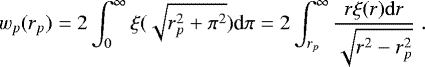
where vp × r is the component of the peculiar velocity of the source along the line of sight. In order to avoid such effects the so-called projected correlation function, wp(rp), can be used to infer the spatial clustering (e.g. Davis & Peebles 1983).
To this end, we deconvolve the redshift-based distance of a source, s, in two components, one parallel (π) and one perpendicular (rp) to the line of sight, i.e.  , and thus the redshift-space correlation function can be written as ξ(s) = ξ(rp, π). Since redshift space distortions affect only the π component, we can estimate the projected correlation function, wp(rp) (which is free of z-space distortions), by integrating ξ(rp, π) along π:
 (2)
(2)
Once we have estimated the projected correlation function, wp (rp), we can recover the real space correlation function since the two are related according to (Davis & Peebles 1983)
 (3)
(3)
Modelling ξ(r) as a power law,  , we obtain
 (4)
(4)
with
 (5)
(5)
where Γ is the usual gamma function.
However, it should be noted that although Eq. (4) strictly holds for πmax = ∞, practically we always impose a cut-off πmax (for reasons discussed in the next section). This introduces an underestimation of the underlying correlation function, which is an increasing function of separation rp. For a power-law correlation function this underestimation is easily inferred from Eq. (3) and is given by (e.g. Starikova et al. 2011)
 (6)
(6)
Thus, by taking into account the above statistical correction, and under the assumption of the power-law correlation function, we can recover the corrected spatial correlation function, ξ(rp), from the fit to the measured wp(rp) according to
 (7)
(7)
which provides also the value of γ. However, at large separations the correction factor increasingly dominates over the signal, and thus it constitutes an unreliable correction procedure.
3.1 Correlation function estimator
As a first step we calculate ξ(rp, π) using the Landy & Szalay (1993) estimator (for a discussion regarding different estimators see Kerscher et al. 2000)
 (8)
(8)
where DD(rp, π), RR(rp, π), and DR(rp, π) are the number of data-data, random-random, and data-random pairs, respectively. We then estimate the redshift-space correlation function, ξ(s), in the comoving redshift separation range s ∈ [1, 80] h−1 Mpc and the projected correlation function, wp(rp), in the comoving projected separation range rp ∈ [0.5, 40] h−1 Mpc. We note that large separations in the π direction mostly add noise to the above estimator and therefore the integration is truncated for separations larger than πmax. The choice of πmax is a compromise between having an optimal signal-to-noise ratio for ξ and reducing theexcess noise from high π separations. The majority of studies in the literature usually assume πmax ∈ [5, 30] h−1 Mpc.
The correlation function uncertainty is estimated according to
 (9)
(9)
which corresponds to that expected by the bootstrap technique (Mo et al. 1992). In this work, we bin the source pairs in logarithmic intervals of δlog10(rp, π) ≃ 0.19 and δlog10(s) ≃ 0.12 for the wp(rp) and ξ(s) correlation functions, respectively. Finally, we use a χ2 minimization procedure between data and the power-law model for either type of the correlation function to derive the best-fit r0 and γ parameters. We carefully choose the range of separations in order to obtain the best power-law fit to the data and we impose a lower separation limit of rp ~ 1 h−1 Mpc to minimize non-linear effects.
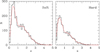 |
Fig. 1 Redshift distribution of the soft and hard XXL-S AGN samples. The red curve corresponds to the mean over 100 random realizations according to the prescription described in Gilli et al. (2005) and using a Gaussian with a smoothing length of σz = 0.125. |
3.2 Random catalogue construction
To estimate the spatial correlation function of a sample of sources we need to construct a large mock comparison sample with a random spatial distribution within the survey area, which also reproduces all the systematic biases that are present in the source sample (i.e. instrumental biases due to the point spread function variation, vignetting, etc.). Also, special care has to be taken to reproduce any biases that enter through the optical counterpart spectroscopic observations strategy (for example, due to fibre collisions in multifibre spectographs or due to the positioning of the slits on the masks in multislit spectrographs, etc.).
To this end we follow the random catalogue construction procedure of Gilli et al. (2005), which is based on reshuffling only the source redshifts, smoothing the corresponding redshift distribution, while keeping the angular coordinates unchanged, thus reproducing all the previously discussed biases. In detail we assign random redshifts to the mock sample by smoothing the source redshift distribution using a Gaussian kernel with a smoothing length of σz = 0.125. This offers a compromise between scales that are either too small and thus may reproduce the z-space clustering, or too large and thus over-smooth the observed redshift distribution, providing an unrealistically high clustering pattern. In Fig. 1 we present the redshift distribution of the soft- and hard-band AGN samples overplotted with the mean over 100 random realizations, according to the above prescription.
We arrived at this value of σz after investigating the effect of different values on the resulting clustering pattern. Interestingly, we found that values in the range 0.05≤ σz ≤ 0.2 provide very consistent clustering results when using the Landy & Szalay (1993) estimator of the 2-p correlation function, while other estimators (e.g. Hamilton 1993) show a large scatter of the clustering results. This is depicted in Fig. 2 where we plot the wp (r) difference between the results based on σz = 0.125 and those indicated within the plot. It is evident that the Landy & Szalay estimator outperforms the corresponding Hamilton estimator by a large margin.
Finally, we note that in the following analysis we have limited our samples to z ≤ 3, since the few higher redshift AGNs, sampling a wide redshift range but extremely sparsely, would act mostly as noise in the clustering analysis.
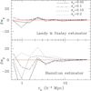 |
Fig. 2 Difference of the projected correlation function, wp(rp), based on a random catalogues constructed with σz = 0.125 with those based on the indicated values of σz. Upper panel: results based on the Landy & Szalay (1993) estimator of the 2-p correlation function. Lower panel: results based on the Hamilton (1993) estimator of the 2-p correlation function. |
4 Results and discussion
We first present results based on the complete sample of sources, spanning all redshifts, with estimated Lx ≳ 1041 erg s−1 cm−2, in order to clearly exclude galaxies. Weselect the optimal πmax cut-off by investigating the performance of the resulting clustering parameters for different values of πmax. We select as our optimal value that for which the clustering parameters show stability. In Fig. 3 we present for both the soft- and hard-band sources the clustering length, rp,0, as a function of πmax for the nominal slope γ = 1.8. We see that for 20 ≲ πmax∕h−1 Mpc ≲ 40 the value of rp,0 is quite stable and equals ≃ 5.6 and ≃ 5.2 h−1 Mpc for the soft- and hard-band sources respectively. For the remaining discussion and results we use consistently πmax = 20 h−1 Mpc.
The derived wp(rp) correlation function is shown in Fig. 4 for both soft- and hard-band sources, while the parameters of the power-law fit, within 1 h−1 Mpc ≲ rp ≲ 25 h−1 Mpc, are shown in Table 1 for both the projected correlation function, wp(rp), and the inferred spatial correlation function (Eq. (7)).
A first important result, indicated both by Fig. 4 and Table 1, is the clustering consistency between the soft- and hard-band sources, although there seems to be a slight but rather insignificant enchancement of the soft-band clustering with respect to that of the hard-band, indicated also in the inset panel by the confidence levels of the fitted correlation function parameters. The inferred spatial correlation length is rp,0 = 7.00 ± 0.34 and 6.42± 0.42 h−1 Mpc for the soft- and hard-band sources, respectively, while for both the slope is γ = 1.44 ± 0.10. We also note the median redshift difference among the two bands.
A second important result is that the inferred clustering is in good agreement with Chandra results, i.e. with the Koutoulidis et al. (2013) clustering analysis of a large compilation of 1466 Chandra 0.5–8 keV sources, which have a median redshift of  , similar to that of our sample, and which provided r0 = 7.2(±0.6) h−1 Mpc and γ = 1.48(±0.12), and with the Starikova et al. (2011) results of the Bootes field (based on the 0.5–2 keV band sources).
In order to visualize the recovery of the true spatial correlation function via Eq. (7), we plot in Fig. 5 the inferred correlation function ξ(rp) together with the redshift-space correlation function, ξ(s) (separately for the soft- and hard-band XXL-S sources) which should be boosted up by redshift-space distortions. Evidently, however, there is an excellent consistency between the two, with both the amplitude and the slope of the power-law fit being in agreement, as can be seen in the insets and in Table 1. We infer that redshift-space distortions do not significantly affect our sample. Furthermore, the inferred spatial clustering lengths correspond to bias values of b ≃ 2.17 ± 0.10 and b ≃ 1.87 ± 0.11 for the soft- and hard-bands at  and 0.79, respectively. These bias values result from (Peebles 1980, 1993)
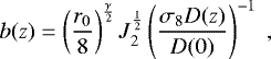 (10)
(10)
where D(z) is the Λ CDM fluctuations growing mode, σ8 = 0.81 is the normalization of the power spectrum (consistent with that of the joint Planck analysis of the Planck Collaboration XIII 2016), and J2(γ) = 72∕[(3 − γ)(4 − γ)(6 − γ)2γ].
We now attempt to investigate the redshift evolution of the AGN correlation function for both the soft- and hard-band sources. To this end we determine the clustering pattern of the following:
the dominant population of XXL-S sources, i.e. those that populate the redshift range around its mode value (0.3 < z < 1.1), which consists of 1375 and 932 soft- and hard-band sources, respectively, with a median redshift of the samples
 ;
;the higher redshift regime, i.e. 1.1 < z < 3, which consists of 1291 soft and 680 hard band sources, respectively, with corresponding median redshifts:
 and 1.63.
The resulting spatial clustering power-law results for the 0.3 < z < 1.1 redshift bin are r0 = 7.10 ± 0.42 h−1 Mpc and γ = 1.45 ± 0.09 for the soft-band and r0 = 5.52 ± 0.54 h−1 Mpc and γ = 1.42 ± 0.12 for the hard-band, respectively. The 1, 2, and 3σ confidence contour levels of the fitted two parameter power-law correlation function model can be seen in Fig. 6. The difference between the soft- and hard-band results is now more pronounced, providing evidence for the reality of the difference. These clustering lengths corresponds to bias values of b ≃ 1.85 ± 0.10 and b ≃ 1.56 ± 0.13, respectively.The results appear to contradict the findings of Elyiv et al. (2012), based on the XMM-LSS, who found that the amplitude of the correlation function is higher in the hard band than in the soft band. A possible explanation is that they do not derive the correlation length directly (due to the absence of spectroscopic redshift information), but use the more uncertain Limbers inversion of the angular clustering pattern.
Analysing the soft-band AGN sample in the higher redshift bin, we find results with a large scatter depending on the separation range used to fit the power-law model to the correlation function; it ranges from ~ 6 to 8 h−1 Mpc and the slope γ from ~1.2 to ~ 2. Using the separation range rp ∈ [3, 35] h−1 Mpc, in order to avoid the large scatter at smaller separations and to enhance our signal, we find r0 = 7.64 ± 0.7 h−1 Mpc and γ = 1.91 ± 0.16, while for a fixed γ = 1.8 we obtain r0 ≃ 7.2 ± 1.0 h−1 Mpc. The measured clustering corresponds to a linear bias factor of b = 3.68 ± 0.46 at  , where the quoted uncertainty also takes into account the r0 scatter due to the separation range used in the power-law fit.
In order to compare our results with those of a large number of recent determinations of the X-ray AGN bias, we present in Fig. 7 the corresponding bias values as a function of redshift. The results of different studies are all translated to the Planck 2015 cosmology (Ωm = 0.3 and σ8 = 0.81) and are indicated by different symbols (as indicated within the figure). The filled green symbols correspond to our current results based on the soft band and the two separate redshift bins, while the open green square corresponds to the overall hard-band results (since we were unable to clearly detect a clustering signal at the high redshift range).
We have fitted two different bias evolution models to the data, the Basilakos et al. (2008) and the Tinker et al. (2010) models, using a χ2 minimization procedure and we derive the DM host halo mass (details and comparisons of the different bias models can be found in Papageorgiou et al. 2012, 2018). We find log10Mh∕[h−1M⊙] = 13.04 ± 0.06 and 12.98 ± 0.07 for the two models, respectively. The corresponding fits can be seen in Fig. 6 as the continous black and broken magenta curves. We note that in the above fit we have excluded the offset results at z ~ 0.75 and by doing so we obtain an excellent fit with a reduced χ2 /d.f. = 0.93. Using all the bias data we obtain the same halo mass, but naturally with a worse reduced χ2.
It is evident that the current results are in agreement with the general trend provided by all previous studies, and consistent with X-ray AGN being hosted by ~ 1013 h−1M⊙ DM halos. The general trend of a significantly higher bias and corresponding host DM halo mass of the X-ray selected AGN with respect to optically selected AGN (e.g. Croom et al. 2005; Ross et al. 2009), which appear to inhabit DM halos with log 10Mh∕[h−1M⊙] ≃ 12.50 ± 0.05 (see e.g. Koutoulidis et al. 2013, and references therein), indicates a different fuelling mechanism for the two populations of AGN.
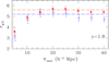 |
Fig. 3 Dependence of the wp(rp) clustering length on the cut-off πmax value for the case of constant slope γ = 1.8. The red filled points correspond to the soft-band results, while the blue open points to the corresponding hard-band results. The red and blue dashed lines correspond to the estimated final rp,0 correlation lengths of the soft- and hard-band sources, respectively. |
Clustering results based on a power-law model fit within 1 < rp < 20 h−1 Mpc, using the whole sample of soft- and hard-band X-ray AGN sources.
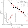 |
Fig. 4 Projected correlation function of the soft (filled points) and hard X-ray AGNs (open red points) for the whole XXL-S AGN sampleand for rp ≳ 1 h−1 Mpc. In the inset panel we only show the 1σ and 3σ confidence contour levels of the corresponding fitted correlation function parameters in order to avoid crowding. |
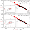 |
Fig. 5 Redshift-space correlation function, ξ(s) (filled circular points), and the inferred real 3D correlation function, ξ(rp) (red pentagons), for the soft- (upper panel) and hard-band XXL-S AGNs (lower panel). The black line corresponds to the power-law fit to ξ(s), and the red line to ξ(rp). The empty circular points signify the small and large separation ξ(s) range that are not used in the power-law fit. In the insets we show the 1, 2, and 3σ confidence contour levels of the corresponding fitted correlation function parameters. |
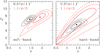 |
Fig. 6 Confidence contour levels (1, 2, and 3σ) of the χ2 fitted two-parameter power-law correlation function model for two redshift ranges, and separately for the soft- and hard-band sources. |
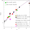 |
Fig. 7 Redshift evolution of the X-ray AGN linear bias factor, as derived from a number of recent studies indicated in the plot. The bias values shown correspond to a flat Λ CDM cosmologicalmodel with Ωm = 0.3 and σ8 = 0.81. The black continuous curve corresponds to the bias evolution model of Basilakos et al. (2008) for a DM host halo mass of Mh = 1013.04h−1M⊙, while the magenta dashed line corresponds to the model of Tinker et al. (2010) for Mh = 1012.96h−1M⊙. |
5 Conclusions
We have analysed the clustering pattern of a homogeneous X-ray AGN spectroscopic sample of the XMM southern field, with a ~ 90% redshift completeness down to an optical counterpart r-band magnitude of 21.8. The sample constitutes the largest spectroscopic sample of X-ray AGN, with a flux limit of ~ 2.2 × 10⁻¹⁵ and ~ 1.4 × 10⁻¹⁴ erg s−1 cm2 (corresponding to 50% of the area curve for the soft band and hard band, respectively), covering a coherent area of ~ 25 deg2.
Our main results are as follows:
The clustering of the X-ray AGN, detected in either soft or hard bands, are well represented by the usual power law in the separation range of 1 ≲ rp ≲ 25 h−1 Mpc, with the inferred spatial clustering length being r0 ≃ 7(±0.3) and 6.4(±0.4) h−1 Mpc for the soft and hard-band detected sources, respectively. The slope for both cases is γ = 1.44(±0.1). The corresponding clustering lengths for the nominal slope γ = 1.8 are r0 ≃ 7.5(±0.3) and ≃ 7.0(±0.4) h−1 Mpc. These results are in good agreement with the analysis of a joint Chandra sample of 1466 sources, having a similar median redshift with our sample, by Koutoulidis et al. (2013) who find r0 ≃ 7.2(±0.6) h−1 Mpc and γ = 1.48(±0.12).
The weak excess clustering of the soft sources with respect to those detected in the hard band becomes more pronounced and significant if we limit our analysis around the mode of the redshift distribution (i.e. 0.3 < z < 1.1), in which case we find the same slope of the power-law, but the clustering lengths become ~ 7.1(±0.4) and ~5.5(±0.5) h−1 Mpc for the soft- and hard-band detected sources, respectively. This is in disagreement with the angular clustering analysis of Elyiv et al. (2012).
The derived linear bias factor at the median redshift of the sample and in two separate redshift bins corresponds to the expectation of host dark matter halos with a mass Mh ≃ 1013h−1 M⊙, in agreement with most recent analysis of local or distant samples of X-ray AGN (e.g. Allevato et al. 2016; Mendez et al. 2016; Krumpe et al. 2018).
Acknowledgements
The Saclay group acknowledges long-term support from the Centre National d’Études Spatiales (CNES). EK thanks CNES and CNRS for their support of post-doctoral research. XXL is an international project based around an XMM Very Large Programme surveying two 25 deg2 extragalactic fields at a depth of ~ 5 × 10⁻¹⁵ erg cm−2 s−1 in the [0.5–2] keV band for point-like sources. The XXL website is http://irfu.cea.fr/xxl. Multi-band information and spectroscopic follow-up of the X-ray sources are obtained through a number of survey programmes, summarised at http://xxlmultiwave.pbworks.com/
References
- Adami, C., Giles, P., Koulouridis, E., et al. 2018, A&A, 620, A5 (XXL Survey, XX) [NASA ADS] [CrossRef] [EDP Sciences] [Google Scholar]
- Alexander, D. M., & Hickox, R. C. 2012, New Astron. Rev., 56, 93 [NASA ADS] [CrossRef] [Google Scholar]
- Allevato, V., Finoguenov, A., Cappelluti, N., et al. 2011, ApJ, 736, 99 [NASA ADS] [CrossRef] [Google Scholar]
- Allevato, V., Civano, F., Finoguenov, A., et al. 2016, ApJ, 832, 70 [NASA ADS] [CrossRef] [Google Scholar]
- Baldry, I. K., Liske, J., Brown, M. J. I., et al. 2018, MNRAS, 474, 3875 [NASA ADS] [CrossRef] [Google Scholar]
- Basilakos, S., Plionis, M., & Ragone-Figueroa, C. 2008, ApJ, 678, 627 [NASA ADS] [CrossRef] [Google Scholar]
- Bertin, E., & Arnouts, S. 1996, A&AS, 117, 393 [NASA ADS] [CrossRef] [EDP Sciences] [Google Scholar]
- Bournaud, F., Dekel, A., Teyssier, R., et al. 2011, ApJ, 741, L33 [NASA ADS] [CrossRef] [Google Scholar]
- Brusa, M., Zamorani, G., Comastri, A., et al. 2007, ApJS, 172, 353 [NASA ADS] [CrossRef] [Google Scholar]
- Cappelluti, N., Ajello, M., Burlon, D., et al. 2010, ApJ, 716, L209 [NASA ADS] [CrossRef] [Google Scholar]
- Cash, W. 1979, ApJ, 228, 939 [NASA ADS] [CrossRef] [Google Scholar]
- Chiappetti, L., Fotopoulou, S., Lidman, C., et al. 2018, A&A, 620, A12 (XXL Survey, XXVII) [NASA ADS] [CrossRef] [EDP Sciences] [Google Scholar]
- Coil, A. L., Georgakakis, A., Newman, J. A., et al. 2009, ApJ, 701, 1484 [NASA ADS] [CrossRef] [Google Scholar]
- Coil, A. L., Hennawi, J. F., Newman, J. A., Cooper, M. C., & Davis, M. 2007, ApJ, 654, 115 [NASA ADS] [CrossRef] [Google Scholar]
- Croom, S. M., Boyle, B. J., Shanks, T., et al. 2005, MNRAS, 356, 415 [NASA ADS] [CrossRef] [Google Scholar]
- Davis, M., & Peebles, P. J. E. 1983, ApJ, 267, 465 [NASA ADS] [CrossRef] [Google Scholar]
- Desai, S., Armstrong, R., Mohr, J. J., et al. 2012, ApJ, 757, 83 [NASA ADS] [CrossRef] [Google Scholar]
- Desai, S., Mohr, J. J., Henderson, R., et al. 2015, J. Instrum., 10, C06014 [CrossRef] [Google Scholar]
- Di Matteo, T., Springel, V., & Hernquist, L. 2005, in Growing Black Holes: Accretion in Cosmological Context, eds. A. Merloni, S. Nayakshin, & R. A. Sunyaev, 345 [Google Scholar]
- Downes, A. J. B., Peacock, J. A., Savage, A., & Carrie, D. R. 1986, MNRAS, 218, 31 [NASA ADS] [CrossRef] [Google Scholar]
- Elyiv, A., Clerc, N., Plionis, M., et al. 2012, A&A, 537, A131 [NASA ADS] [CrossRef] [EDP Sciences] [Google Scholar]
- Fanidakis, N., Baugh, C. M., Benson, A. J., et al. 2012, MNRAS, 419, 2797 [NASA ADS] [CrossRef] [Google Scholar]
- Fanidakis, N., Georgakakis, A., Mountrichas, G., et al. 2013, MNRAS, 435, 679 [NASA ADS] [CrossRef] [Google Scholar]
- Flaugher, B., Diehl, H. T., Honscheid, K., et al. 2015, AJ, 150, 150 [NASA ADS] [CrossRef] [Google Scholar]
- Fotopoulou, S., Pacaud, F., Paltani, S., et al. 2016, A&A, 592, A5 (XXL Survey, VI) [NASA ADS] [CrossRef] [EDP Sciences] [Google Scholar]
- Gilli, R., Daddi, E., Zamorani, G., et al. 2005, A&A, 430, 811 [NASA ADS] [CrossRef] [EDP Sciences] [Google Scholar]
- Gilli, R., Zamorani, G., Miyaji, T., et al. 2009, A&A, 494, 33 [NASA ADS] [CrossRef] [EDP Sciences] [Google Scholar]
- Gültekin, K., Richstone, D. O., Gebhardt, K., et al. 2009, ApJ, 698, 198 [NASA ADS] [CrossRef] [Google Scholar]
- Hale, C. L., Jarvis, M. J., Delvecchio, I., et al. 2018, MNRAS, 474, 4133 [NASA ADS] [CrossRef] [Google Scholar]
- Hamilton, A. J. S. 1993, ApJ, 417, 19 [NASA ADS] [CrossRef] [Google Scholar]
- Hickox, R. C., Jones, C., Forman, W. R., et al. 2009, ApJ, 696, 891 [Google Scholar]
- Hopkins, P. F., & Hernquist, L. 2006, ApJS, 166, 1 [NASA ADS] [CrossRef] [Google Scholar]
- Hopkins, P. F., Hernquist, L., Cox, T. J., et al. 2006, ApJS, 163, 1 [Google Scholar]
- Kerscher, M., Szapudi, I., & Szalay, A. S. 2000, ApJ, 535, L13 [NASA ADS] [CrossRef] [PubMed] [Google Scholar]
- Koulouridis, E., Poggianti, B., Altieri, B., et al. 2016, A&A, 592, A11 (XXL Survey, XII) [NASA ADS] [CrossRef] [EDP Sciences] [Google Scholar]
- Koutoulidis, L., Plionis, M., Georgantopoulos, I., & Fanidakis, N. 2013, MNRAS, 428, 1382 [NASA ADS] [CrossRef] [Google Scholar]
- Krumpe, M., Miyaji, T., & Coil, A. L. 2010, ApJ, 713, 558 [NASA ADS] [CrossRef] [Google Scholar]
- Krumpe, M., Miyaji, T., Coil, A. L., & Aceves, H. 2018, MNRAS, 474, 1773 [NASA ADS] [CrossRef] [Google Scholar]
- Landy, S. D., & Szalay, A. S. 1993, ApJ, 412, 64 [NASA ADS] [CrossRef] [Google Scholar]
- Lidman, C., Ardila, F., Owers, M., et al. 2016, PASA, 33, e001 [NASA ADS] [CrossRef] [Google Scholar]
- Magliocchetti, M., Popesso, P., Brusa, M., et al. 2017, MNRAS, 464, 3271 [NASA ADS] [CrossRef] [Google Scholar]
- Magorrian, J., Tremaine, S., Richstone, D., et al. 1998, AJ, 115, 2285 [NASA ADS] [CrossRef] [Google Scholar]
- Marulli, F., Bonoli, S., Branchini, E., et al. 2009, MNRAS, 396, 1404 [NASA ADS] [CrossRef] [Google Scholar]
- Mendez, A. J., Coil, A. L., Aird, J., et al. 2016, ApJ, 821, 55 [NASA ADS] [CrossRef] [Google Scholar]
- Miyaji, T., Krumpe, M., Coil, A. L., & Aceves, H. 2011, ApJ, 726, 83 [NASA ADS] [CrossRef] [Google Scholar]
- Mo, H. J., Jing, Y. P., & Boerner, G. 1992, ApJ, 392, 452 [NASA ADS] [CrossRef] [Google Scholar]
- Mountrichas, G., Georgakakis, A., Menzel, M.-L., et al. 2016, MNRAS, 457, 4195 [NASA ADS] [CrossRef] [Google Scholar]
- Mullis, C. R., Henry, J. P., Gioia, I. M., et al. 2004, ApJ, 617, 192 [NASA ADS] [CrossRef] [Google Scholar]
- Pacaud, F., Clerc, N., Giles, P. A., et al. 2016, A&A, 592, A2 (XXL Survey, II) [NASA ADS] [CrossRef] [EDP Sciences] [Google Scholar]
- Pacaud, F., Pierre, M., Refregier, A., et al. 2006, MNRAS, 372, 578 [NASA ADS] [CrossRef] [Google Scholar]
- Papageorgiou, A., Basilakos, S., & Plionis, M. 2018, MNRAS, 476, 2621 [NASA ADS] [CrossRef] [Google Scholar]
- Papageorgiou, A., Plionis, M., Basilakos, S., & Ragone-Figueroa, C. 2012, MNRAS, 422, 106 [NASA ADS] [CrossRef] [Google Scholar]
- Peebles, P. J. E. 1980, The Large-Scale Structure of the Universe (Princetown: Princetown University Press) [Google Scholar]
- Peebles, P. J. E. 1993, Principles of Physical Cosmology (Princetown: Princetown University Press) [Google Scholar]
- Pierre, M., Pacaud, F., Adami, C., et al. 2016, A&A, 592, A1 (XXL Survey, I) [NASA ADS] [CrossRef] [EDP Sciences] [Google Scholar]
- Planck Collaboration XIII. 2016, A&A, 594, A13 [NASA ADS] [CrossRef] [EDP Sciences] [Google Scholar]
- Plionis, M., Rovilos, M., Basilakos, S., Georgantopoulos, I., & Bauer, F. 2008, ApJ, 674, L5 [NASA ADS] [CrossRef] [Google Scholar]
- Ross, N. P., Shen, Y., Strauss, M. A., et al. 2009, ApJ, 697, 1634 [NASA ADS] [CrossRef] [Google Scholar]
- Scodeggio, M., Guzzo, L., Garilli, B., et al. 2018, A&A, 609, A84 [NASA ADS] [CrossRef] [EDP Sciences] [Google Scholar]
- Starck, J.-L., & Pierre, M. 1998, A&AS, 128, 397 [NASA ADS] [CrossRef] [EDP Sciences] [Google Scholar]
- Starikova, S., Cool, R., Eisenstein, D., et al. 2011, ApJ, 741, 15 [Google Scholar]
- Sutherland, W., & Saunders, W. 1992, MNRAS, 259, 413 [NASA ADS] [CrossRef] [Google Scholar]
- Tinker, J. L., Robertson, B. E., Kravtsov, A. V., et al. 2010, ApJ, 724, 878 [NASA ADS] [CrossRef] [Google Scholar]
- Yang, Y., Mushotzky, R. F., Barger, A. J., & Cowie, L. L. 2006, ApJ, 645, 68 [NASA ADS] [CrossRef] [Google Scholar]
- Zubovas, K., & King, A. R. 2012, MNRAS, 426, 2751 [NASA ADS] [CrossRef] [Google Scholar]
All Tables
Clustering results based on a power-law model fit within 1 < rp < 20 h−1 Mpc, using the whole sample of soft- and hard-band X-ray AGN sources.
All Figures
|
Fig. 1 Redshift distribution of the soft and hard XXL-S AGN samples. The red curve corresponds to the mean over 100 random realizations according to the prescription described in Gilli et al. (2005) and using a Gaussian with a smoothing length of σz = 0.125. |
| In the text | |
|
Fig. 2 Difference of the projected correlation function, wp(rp), based on a random catalogues constructed with σz = 0.125 with those based on the indicated values of σz. Upper panel: results based on the Landy & Szalay (1993) estimator of the 2-p correlation function. Lower panel: results based on the Hamilton (1993) estimator of the 2-p correlation function. |
| In the text | |
|
Fig. 3 Dependence of the wp(rp) clustering length on the cut-off πmax value for the case of constant slope γ = 1.8. The red filled points correspond to the soft-band results, while the blue open points to the corresponding hard-band results. The red and blue dashed lines correspond to the estimated final rp,0 correlation lengths of the soft- and hard-band sources, respectively. |
| In the text | |
|
Fig. 4 Projected correlation function of the soft (filled points) and hard X-ray AGNs (open red points) for the whole XXL-S AGN sampleand for rp ≳ 1 h−1 Mpc. In the inset panel we only show the 1σ and 3σ confidence contour levels of the corresponding fitted correlation function parameters in order to avoid crowding. |
| In the text | |
|
Fig. 5 Redshift-space correlation function, ξ(s) (filled circular points), and the inferred real 3D correlation function, ξ(rp) (red pentagons), for the soft- (upper panel) and hard-band XXL-S AGNs (lower panel). The black line corresponds to the power-law fit to ξ(s), and the red line to ξ(rp). The empty circular points signify the small and large separation ξ(s) range that are not used in the power-law fit. In the insets we show the 1, 2, and 3σ confidence contour levels of the corresponding fitted correlation function parameters. |
| In the text | |
|
Fig. 6 Confidence contour levels (1, 2, and 3σ) of the χ2 fitted two-parameter power-law correlation function model for two redshift ranges, and separately for the soft- and hard-band sources. |
| In the text | |
|
Fig. 7 Redshift evolution of the X-ray AGN linear bias factor, as derived from a number of recent studies indicated in the plot. The bias values shown correspond to a flat Λ CDM cosmologicalmodel with Ωm = 0.3 and σ8 = 0.81. The black continuous curve corresponds to the bias evolution model of Basilakos et al. (2008) for a DM host halo mass of Mh = 1013.04h−1M⊙, while the magenta dashed line corresponds to the model of Tinker et al. (2010) for Mh = 1012.96h−1M⊙. |
| In the text | |
Current usage metrics show cumulative count of Article Views (full-text article views including HTML views, PDF and ePub downloads, according to the available data) and Abstracts Views on Vision4Press platform.
Data correspond to usage on the plateform after 2015. The current usage metrics is available 48-96 hours after online publication and is updated daily on week days.
Initial download of the metrics may take a while.