| Issue |
A&A
Volume 619, November 2018
|
|
|---|---|---|
| Article Number | A135 | |
| Number of page(s) | 12 | |
| Section | Extragalactic astronomy | |
| DOI | https://doi.org/10.1051/0004-6361/201833841 | |
| Published online | 15 November 2018 | |
Dust attenuation and Hα emission in a sample of galaxies observed with Herschel at 0.6 < z < 1.6
1
Aix Marseille Univ, CNRS, CNES, LAM
Marseille, France
e-mail: veronique.buat@lam.fr
2
Centro de Astronomía (CITEVA), Universidad de Antofagasta, Avenida Angamos 601, Antofagasta, Chile
3
National Centre for Nuclear Research, ul. Hoza 69, 00-681
Warszawa, Poland
4
Univ. Lyon1, ENS de Lyon, CNRS, Centre de Recherche Astrophysique de Lyon UMR5574, 69230
Saint-Genis-Laval, France
5
Astronomy Centre, Department of Physics and Astronomy, University of Sussex, Falmer, Brighton
BN1 9QH , UK
6
School of Sciences, European University Cyprus, Diogenes Street, Engomi, 1516
Nicosia, Cyprus
Received:
13
July
2018
Accepted:
28
August
2018
Context. Dust attenuation shapes the spectral energy distribution of galaxies. It is particularly true for dusty galaxies in which stars experience a heavy attenuation. The combination of UV to IR photometry with the spectroscopic measurement of the Hα recombination line helps to quantify dust attenuation of the whole stellar population and its wavelength dependence.
Aims. We want to derive the shape of the global attenuation curve and the amount of obscuration affecting young stars or nebular emission and the bulk of the stellar emission in a representative sample of galaxies selected in IR. We will compare our results to the commonly used recipes of Calzetti et al. and Charlot and Fall, and to predictions of radiative transfer models.
Methods. We selected an IR complete sample of galaxies in the COSMOS 3D-HST CANDELS field detected with the Herschel satellite with a signal to noise ratio larger than five. Optical to NIR photometry is available as well as NIR spectroscopy for each source. We reduced the sample to the redshift range 0.6 < z < 1.6 to include the Hα line in the G141 grism spectra. We have used a new version of the CIGALE code to fit simultaneously the continuum and Hα line emission of the 34 selected galaxies.
Results. Using flexible attenuation laws with free parameters, we are able to measure the shape of the attenuation curve for each galaxy as well as the amount of attenuation of each stellar population, the former being in general steeper than the starburst law in the UV-optical with a large variation of the slope among galaxies. The attenuation of young stars or nebular continuum is found on average about twice the attenuation affecting older stars, again with a large variation. Our model with power-laws, based on a modification of the Charlot and Fall recipe, gives results in better agreement with the radiative transfer models than the global modification of the slope of the Calzetti law.
Key words: dust, extinction / infrared: galaxies / galaxies: ISM / galaxies: high-redshift
© ESO 2018
1. Introduction
Modeling the spectral energy distribution (SED) of galaxies is a method commonly used to derive physical parameters useful to quantify galaxy evolution, the most popular ones being the star formation rate (SFR) and the stellar mass (Mstar ). The basics of these methods is to reconstruct the stellar emission of a galaxy with population synthesis models and star formation histories (SFHs) of varying complexity with free parameters (e.g., Walcher et al. 2011; Conroy 2013). Dust plays a crucial role by strongly affecting and reshaping the SED: it absorbs and scatters stellar photons, and thermally emits the absorbed energy in the infrared (IR) (λ ~ 1−1000 μm). As a consequence any SED modeling must account for dust attenuation. The easiest way to do this is to introduce a single attenuation curve which accounts for the complex blending of dust properties and relative geometrical distribution of stars and dust within a galaxy. The attenuation law built by Calzetti and collaborators for nearby starburst galaxies (Calzetti et al. 1994, 2000) is by far the most commonly used. It is characterized by a grayer slope than both Milky Way and Large Magellanic Cloud extinction curves and by the lack of the so-called UV bump corresponding to the 2175 Å absorption feature. Charlot & Fall (2000) proposed a recipe also implemented in SED fitting codes. This recipe was originally built to be consistent with the properties of the nearby starburst galaxies analyzed by Calzetti et al. (1994) but both recipes differ substantially in the visible to near-IR (NIR; Chevallard et al. 2013; Lo Faro et al. 2017; Malek et al. 2018).
The universality of an attenuation recipe remains an open question in the nearby universe as well as for more distant galaxies. Battisti et al. (2016, 2017) combined ultraviolet (UV) photometric data from GALEX with SDSS spectroscopy and NIR data from the UKIRT and 2MASS surveys for several thousands of local galaxies, deriving an attenuation curve similar to the starburst law although slightly lower in the UV. Conversely Salim et al. (2018) extended the GALEX and SDSS data to the IR, with WISE and Herschel detections and concluded that there is a high variety of attenuation curves whose slope is a strong function of optical opacity confirming the results of radiative transfer calculations (e.g., Witt & Gordon 2000; Pierini et al. 2004; Tuffs et al. 2004; Inoue 2005; Panuzzo et al. 2007; Chevallard et al. 2013; Seon & Draine 2016).
At higher redshift Reddy et al. (2015) found an average attenuation curve of z ~ 2 galaxies similar to the law of Calzetti et al. (2000) in the UV. More recently Cullen et al. (2018) also obtained an attenuation curve similar in shape to the starburst law for z ~ 3.5 star-forming galaxies. However Salmon et al. (2016) presented strong statistical evidence for the non universality of dust attenuation laws at z ~ 2. Lo Faro et al. (2017) derived flat attenuation curves for ultra luminous IR galaxies (ULIRGs). Both observational and modeling analyses of the infrared excess (IRX) versus the UV spectral slope also support the variability of the attenuation curve of star forming galaxies from steep shapes for young, low-mass galaxies to grayer curves for IR bright, dusty galaxies (e.g., Salmon et al. 2016; Lo Faro et al. 2017; Popping et al. 2017; Narayanan et al. 2018).
When stellar continuum and nebular line emissions are considered together, both must be corrected for dust attenuation and a differential attenuation has been introduced by Calzetti et al. (2000) and Charlot & Fall (2000). The relative attenuation affecting distinct populations and their related emission remains an open issue as does the attenuation law to apply to each component (e.g., Garn et al. 2010; Wild et al. 2011; Chevallard et al. 2013; Kashino et al. 2013; Price et al. 2014; Reddy et al. 2015; Lo Faro et al. 2017; Theios et al. 2018). The difference found between the attenuation of nebular lines on one side and the continuum stellar population on the other side by Calzetti et al. (2000) in nearby starbursts was confirmed by several studies at higher redshifts (Garn et al. 2010; Price et al. 2014) but other analyses found a more similar attenuation for young and old populations (Pannella et al. 2015; Puglisi et al. 2016). Large variations were measured among galaxies by Reddy et al. (2015), correlating with the sSFR of the galaxies.
A widespread method to measure a differential attenuation is to assume the attenuation law of Calzetti et al. (2000) and to compare different measures of SFR obtained with UV, IR and Hα emission separately (Garn et al. 2010; Mancini et al. 2011; Wuyts et al. 2011; Puglisi et al. 2016). Indeed, the simultaneous fit of combined spectroscopic and photometric data ensures a full consistency between the available data but is not trivial to perform. A major issue is the sampling difference between spectra (even of low or moderate resolution) and photometric fluxes: the number of spectroscopic data overwhelms the photometric ones. It makes it very difficult to find any meaningful calculation of the likelihood, on which Bayesian methods rely to build the probability density functions of parameters (Pacifici et al. 2012). Methods using Monte Carlo codes are now developed to simultaneously fit full resolution spectroscopy and photometry (Chevallard & Charlot 2016; Fossati et al. 2018). An alternative approach is to extract some spectroscopic information like equivalent widths (Pacifici et al. 2015), fluxes of emission lines, or age-sensitive spectral indices (Boselli et al. 2016), which are added to the input photometric data. This puts stronger constraints on the different stellar populations as well as the amount of dust attenuation while avoiding the oversampling of full spectra.
In this work we aim at fully characterizing dust attenuation for an IR complete sample of galaxies for which 3D-HST spectra cover the wavelength range of the Hα line (Momcheva et al. 2016). We select galaxies in the COSMOS field detected by Herschel (Pilbratt et al. 2010), with either PACS (Poglitsch et al. 2010) or SPIRE (Griffin et al. 2010) instrument, at least in two bands with a signal to noise ratio (S/N) larger than 5. It ensures a good measure of the total IR emission, which is crucial to measure both SFR and dust attenuation robustly. Photometric data from Laigle et al. (2016) and spectroscopic data from the 3D-HST survey are then added. Ensuring an Hα observation for all the sources limits the redshift range from 0.6 to 1.6. The photometric data and Hα fluxes are simultanously fitted with an updated version of the CIGALE fitting code. This homogenous fit is used to derive attenuation curves and differential attenuation characteristics.
The construction of the dataset is detailed in Sect. 2. We describe our SED fitting method and the various attenuation recipes adopted in this study in Sect. 3. The results of our analysis are presented in Sect. 4 and discussed in Sect. 5. A summary of the main results of this work is presented in Sect. 6.
2. Data selection in the COSMOS field
2.1. Target selection
The HELP1 collaboration provides homogeneous and calibrated multiwavelength data over the Herschel Multitiered Extragalactic Survey (HerMES; Oliver et al. 2012) and the H-ATLAS survey (Eales et al. 2010) and some additional fields. This unique dataset which covers several hundred of square degrees is perfectly suited to build multiwavelength datasets with well controlled selection functions. When combining data over a very large range of wavelengths, the source identification becomes a major issue due to the different spatial resolution and source confusion. It is particularly true for Herschel data with a beam reaching 36 arcsec at 500 μm. The strategy adopted by HELP is to build a master list catalog of objects as complete as possible for each field (Shirley et al., in prep.) and to use the NIR sources of this catalog as prior information for the Herschel maps. The XID+ tool (Hurley et al. 2017) uses a Bayesian probabilistic framework and works with prior positions. The code calculates the full posterior probability distribution on flux estimates. At the end a flux is measured, in a probabilistic sense, for all the NIR sources of the master list.
In an early phase of the HELP project, the COSMOS field was chosen for a pilot study. XID+ was run on Spitzer MIPS1, Herschel SPIRE and PACS maps with prior Spitzer IRAC positions for 694478 sources with fluxes greater than 1 μJy in any of the IRAC bands from the COSMOS2015 catalog of Laigle et al. (2016). From this initial catalog we selected sources with at least either two PACS (at 100 and 160 μm) or two SPIRE (at 250 and 350 μm) fluxes with a S/N > 5. The flux measurements satisfied the criterion of goodness defined in XID+ and corresponding to a gaussian posterior distribution of the estimated flux (Hurley et al. 2017). We were left with a sample of 2774 galaxies for the two deg2 of the COSMOS field.
We crossmatched our selected sources with the 3D-HST catalog of the v4.1.5 release with WFC3 G141 grism spectroscopy over 122.2 arcmin2 in the COSMOS field (Momcheva et al. 2016; Brammer et al. 2012). We took the best match within 2 arcsec from the IRAC coordinates of our IR sources. 52 matches were found which correspond to our full Herschel selection within the area covered by the HST grism survey (122.2 arcmin2 against two deg2 covered by the COSMOS2015 catalog): we got a complete IR selected sample with 3D-HST spectra for each source, all but one (resp two) sources are detected with PACS (resp SPIRE). We assigned a red-shift to each source with the z best value defined in the 3D-HST (Cosmos-3dhst.v4.1.5.zfit.linematch) catalog. z best corresponds to a groundbased spectroscopic redshift for 11 sources and to the best fit grism redshift for 39 sources. Two galaxies have only a photometric redshift, they are classified as active galactic nuclei (AGN) and are excluded (see below). Since we are interested in Hα line measurements we restricted the sample to the redshift range 0.6–1.6 where this line is observed with the G141 grism. 37 objects fulfill this condition. Then we excluded three sources classified as AGN from the Chandra Cosmos Legacy Survey2. We are left with 34 galaxies, all but one galaxy, not detected with SPIRE, have PACS and SPIRE fluxes.
2.2. Photometric data
Starting with the multiwavelength catalog of Laigle et al. (2016), COSMOS2015, we add photometry from CFHTLS and CFHT-WIRDS (Megacam bands u, g, r, i, z and WIRcam bands J, H, Ks ), HSC-UDEEP and UDEEP (Hyper-Suprime-Cam bands g, r, i, z, y) and UKIDSS-LAS (WFCAM bands J, H, K) catalogs. We do this such that the final catalog has one measurement per band per camera, that is taking the order above we add measurements if and only if the object does not already have one in the given band from the given camera. The merging strategy is the same as described in Shirley et al. (in prep.) for the ELAIS-N1 field and is detailed in the “dmu1_ml_COSMOS” product available on the Github repository of the project3. The best crossmatching radii are found to be 0.8 arcsec for CFHTLS, HSC-UDEEP and DEEP, and UKIDS, and 1 arcsec for CFHTWIRDS.
For the SED fitting with CIGALE we use only one measurement per band in order to avoid biasing the fit to parts of the spectrum with multiple cameras covering that band. We choose the ordering based on average depth on a given camera. This ordering, defining which camera measurement is preferred is: Megacam, Hyper-Suprime-Cam, VISTA, WIRCAM, WFCAM. For our 34 galaxies, all the photometric data come from the COSMOS2015 catalog. The photometric dataset consists of 16 bands from GALEX NUV to Spitzer MIPS1 and of the 5 bands from Herschel PACS and SPIRE. With the Hα fluxes we get 22 measurements per object. The near-UV (NUV) flux is measured for only 24 sources, all the other bands are available for the whole sample, except for one galaxy without any SPIRE flux. The transmission curves of the filters are presented in Fig. 1 as well as the wavelength coverage on a template SED for the two extreme redshifts of our sample (z = 0.6 and 1.6).
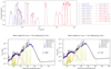 |
Fig. 1. Upper panel: transmission curves of the filters used to build the SED of galaxies, the list of the filters is on the right side of the figure. Lower panel: template SED generated with CIGALE at z = 0.6 and z = 1.6. The solid line is the SED computed with the same modules as the ones used for the fits, with a single model of star formation, dust attenuation and reemission. The red points are the values of the fluxes in the filters whose transmission curves are plotted in the upper panel, the blue squares are mock observations generated by the code with an error of 10% (blue vertical lines, at 3σ). The fluxes are calculated for a total star formation of one solar mass (standard mode for the generation of models with CIGALE). |
2.3. Spectroscopic data
We take the Hα fluxes from the 3D-HST survey4. van Dokkum et al. (2011) showed that for a Hα equivalent width larger than 10 Å, the line is securely measured, without a significant contribution of the underlying stellar absorption. This absorption is directly taken into account in the measurement of the equivalent width (Momcheva et al. 2016) but in case of a faint emission line its contribution is large and increases the uncertainty on the flux measurement. The Hα line is detected with S/N < 2 for three of our sources, and the observed equivalent width of two of these sources is lower than 10 Å, all the others sources have equivalent widths larger than 10 Å. The 3D-HST spectral resolution is not sufficient to detect separately the Hα and the [NII] lines. For the sake of simplicity, hereafter we will refer as Hα fluxes the sum of the Hα and the two [NII] lines.
In this work we analyze individual spectral energy distributions in order to keep the diversity of the sources and we do not stack the data. The Hβ line is not detected on individual sources and we cannot measure Balmer decrements to directly estimate the dust attenuation affecting the Balmer lines (e.g., Garn & Best 2010; Price et al. 2014). The dust emission of our galaxies is measured thanks to the Herschel data and puts a strong constraint on the stellar obscuration through the energy budget between stellar and dust emissions as explained in the next section.
3. The SED fitting method
3.1. The code CIGALE
The SED fitting is performed with the CIGALE code5. We refer to Boquien et al. (2018) and to the description on the web site of CIGALE for more details about the code. CIGALE combines a UV to NIR stellar SED with a dust component emitting in the IR and conserves the energy balance between dust absorbed emission and its thermal reemission. The nebular emission is added from the Lyman continuum photons produced by the stellar component. The nebular continuum and the emission lines are calculated from a grid of nebular templates (Inoue 2011) generated with CLOUDY 08.0. The intensity of 124 lines are included, the models are parametrized with the ionization parameter and the metallicity. Star formation histories as well as dust attenuation recipes can be taken either free or fixed. The global quality of the fit is assessed by a reduced χ
2 ( ) defined as the χ
2 divided by the number of input fluxes. This definition does not account for the degree of freedom of the fit, this quantity is difficult to determine since the free parameters are not independent and the equations linking them are non linear (Chevallard & Charlot 2016). The
) defined as the χ
2 divided by the number of input fluxes. This definition does not account for the degree of freedom of the fit, this quantity is difficult to determine since the free parameters are not independent and the equations linking them are non linear (Chevallard & Charlot 2016). The  value is only used as an indication of the global quality of the fit and the best model is not used for the estimation of the parameters. Instead, the values of the parameters and the corresponding uncertainties are estimated by taking the likelihood weighted mean and standard deviation, the probability distribution function (PDF) of each parameter are built. Here, we only describe the assumptions and choices specific to our current study.
For the purpose of this work, CIGALE is modified (version 0.12.1) so that photometric and emission line fluxes (here only the Hα line) fluxes are fitted simultaneously.
We assume a delayed SFH with the functional form SFR ∝ t exp(−t/τ). A recent constant burst of star formation is overimposed whose amplitude is measured by the stellar mass fraction produced during the burst. This functional SFH is found to give satisfactory results for the galaxies of the ELAIS-N1 field and is routinely used to fit all the HELP samples (Malek et al. 2018). We adopt a Salpeter Initial Mass Function (Salpeter 1955) and the stellar models of Bruzual & Charlot (2003). The metallicity is fixed to the solar value. The input values characterizing the SFH are presented in Table 1.
CIGALE modules and input parameters used for all the fits.
3.2. Parametric attenuation laws
The major aim of this work is to analyze the dust attenuation and its variability among galaxies. Different attenuation recipes are implemented in CIGALE and we start here with two of the most popular ones.
The first recipe we consider is based on the attenuation law for the stellar continuum of Calzetti et al. (2000). The nebular component (and therefore the Hα line) is extinguished with a simple screen model, a Milky Way extinction curve (Cardelli et al. 1989) and a color excess E(B − V)line. The input parameters used to quantify the amount of attenuation are the color excess to apply to the nebular emission, E(B − V)line, and the ratio E(B − V)star/E(B − V)line, E(B − V)star is the color excess to apply to the whole stellar continuum. This ratio was found equal to 0.44 for local starbursts (Calzetti 2001). As we discussed in the introduction, the variability of this ratio is questioned and this parameter is taken free in our fitting procedure. This attenuation recipe (attenuation law of Calzetti et al. (2000), Milky Way extinction curve for the nebular component, and a variable ratio of color excesses) will be called C00 hereafter.
The second recipe we consider is similar to the one proposed by Charlot & Fall (2000). It differs from C00 in its philosophy. A differential attenuation between young (age < 107 years) and old (age > 107 years) stars is assumed. Both young and old stars undergo an attenuation in the interstellar medium (ISM), the young stars are affected by an extra attenuation in the birth clouds (BC). Both attenuation laws are modeled by a power law and normalized to the amount of attenuation in the V band,  and
and  ,
, (1)
(1)
 (2)
(2)
Charlot & Fall (2000) fixed both exponents of the power laws n
BC and n
ISM to −0.7, although a value of −1.3 is initially introduced in their model and further adopted by da Cunha et al. (2008). μ is defined as the ratio of the attenuation in the V band experimented by old and young stars: (3)
(3)
Charlot & Fall (2000) obtained μ = 0.3 from their study of nearby starburst galaxies. As for the ratio of the color excess in the C00 recipe, we take μ as a free parameter in our fits. The recipe defined with the the exponents of the power laws n BC and n ISM equal to −0.7 and μ taken free will be refered as CF00 here-after.
We further introduce some flexibility in the previous recipes and allow the general shape of the attenuation law to be steeper or flatter than the original ones. CF00 becomes the Double Power Law with free slopes (hereafter DBPL-free, as introduced by Lo Faro et al. 2017): n
BC and n
ISM are considered as free parameters. C00 is also modified and we define the Calzetti-like recipe (Noll et al. 2009): (4)
(4)
k′(λ) comes from C00, δ is a free parameter.
In Eq. (4), δ = 0 corresponds to the original recipe C00 and E(B − V)star is equal to AB − AV . When δ ≠ 0, E(B − V)star from Eq. (4) is no longer equal to AB − AV . To avoid a wrong definition, the Calzetti-like recipe is implemented in CIGALE in order that the input parameter E(B − V)star is always equal to AB − AV , for any value of (Boquien et al. 2018). We adopt a fine sampling of the input parameters related to dust attenuation (Table 1) in order to get reliable PDFs, mean values and standard deviations.
3.3. Fitting the SEDs
The modules used for the fits and all their input values are summarized in Table 1. The dust component is calculated with the Draine & Li (2007) models. We use the standard set of parameters adopted for our previous studies of galaxies at similar red-shift and selected in IR (Lo Faro et al. 2017; Malek et al. 2018). In this work we will not focus on the detailed IR emission, we are only interested in the measure of the total IR emission to perform the energy budget of the stellar photons absorbed and reemitted by dust.
The values of  for the different attenuation recipes (CF00, C00, DBPL-free and Calzetti-like) are plotted in Fig. 2. The global quality of the fits is good, in particular with the flexible recipes DBPL-free and Calzetti-like, we will go back to the comparison of the models in the next section.
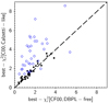 |
Fig. 2. Comparison of the quality of the fits with the four attenuation recipes considered. The best |


The SFR and dust luminosities are found to be similar with all the attenuation recipes with median differences lower than 0.05 dex as illustrated in Fig. 3 for the SFR values obtained with the flexible recipes. The dust luminosity spans only one decade (1011−1012 L ⊙). The mass fraction produced during the current burst is found very low, at most equal to 1%: a single delayed star formation describes the SFH of our galaxies quite well. The stellar masses (M star) exhibit significant differences between models as already underlined by Lo Faro et al. (2017): M star is found higher with CF00 and DBPL-free recipes because of a flatter attenuation curve in the visible to NIR as it will be shown in Sect. 4. The Mstar values obtained with the two flexible recipes are compared in Fig. 3, the median difference reaches 0.27 dex between DBPL-free and Calzetti-like recipes (0.22 dex between CF00 and C00 recipes). When fixed and flexible recipes are compared, the median difference is much lower (0.13 dex between C00 and Calzetti-like, 0.05 dex between CF00 and DBPL-free). The SFR and M star values for our galaxies obtained with the Calzetti-like and DBPL-free recipes are plotted in Fig. 4 together with the average relations of Schreiber et al. (2015) for main sequence (MS) galaxies in the same redshift range. The shift towards lower masses of the values obtained with the Calzettilike method implies that the galaxies exhibit larger specific SFR (SFR divided by stellar mass, hereafter sSFR). At a given stellar mass no galaxy of our sample is found above the MS by more than a factor of 4, which corresponds to the definition of a starburst according to (e.g., Rodighiero et al. 2011; Sargent et al. 2012). We conclude that none of our galaxies is starbursting, in agreement with the delayed SFH.
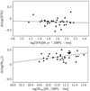 |
Fig. 3. Comparison of SFR and Mstar for the two flexible recipes. The values along the x axis are obtained with the DBPL-free model, the difference between the DBPL-free and Calzetti-like models is plotted on the y axis (DBPL-free minus Calzetti-like logarithmic values). The solid lines are the result of a linear regression. |
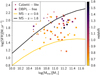 |
Fig. 4. SFR plotted against Mstar for the two flexible recipes DBPL-free (filled squares) and Calzetti-like (dots). The relations of Schreiber et al. (2015) for redshift z = 0.6 and z = 1.6 are represented with solid lines, the redshift of the sources is color coded |
When the DBPL-free recipe is used, it is not possible to estimate securely n BC as already shown by Lo Faro et al. (2017) and we fix its value to −0.7, we checked that using −1.3 does not modify any of the results of this study. The distribution of the total attenuation in the V band is plotted in Fig. 5 for the two flexible recipes, similar distributions are found with the recipes CF00 and C00.
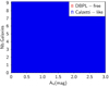 |
Fig. 5. Distribution of the total attenuation in the V band, for DBPL-free (filled red histogram) and Calzetti-like (blue empty histogram). |
4. The derived attenuation laws
4.1. Testing the original recipes of Charlot & Fall (2000) and Calzetti et al. (2000)
We first compare the results of the runs with the original recipes C00 and CF00 (Fig. 2). The fits are significantly better with CF00 with a median value of  equal to 1.57 against 3.32 for C00.
The fits are improved when the slope of the attenuation law is taken free and both recipes return fits of similar quality with a median  of 1.35 and 1.45 for DBPL-free and Calzetti-like recipes respectively. An improvement of the fits is expected since an additional free parameter is introduced in each recipe. However the reduction of
  is stronger in the case of the Calzetti recipe, the CF00 modeling giving satisfactory results already in its original form. This is confirmed by the comparison of the values of the bayesian information criterion (BIC) which accounts for the increase of free parameters6. The difference between BICC00 and BICCalzetti−like is found higher than 6 (which corresponds to a strong evidence against the model with the higher BIC) for 85% of the sample, it drops to 44% between BICCF00 and BICDBPL
−
free. It implies that the global shape of the attenuation curves resulting from the CF00 recipe is more adapted to our galaxy sample than the C00 attenuation law as also found by Lo Faro et al. (2017) and Malek et al. (2018) on different HELP selected samples. In the following we continue the analysis using the flexible attenuation recipes.
is stronger in the case of the Calzetti recipe, the CF00 modeling giving satisfactory results already in its original form. This is confirmed by the comparison of the values of the bayesian information criterion (BIC) which accounts for the increase of free parameters6. The difference between BICC00 and BICCalzetti−like is found higher than 6 (which corresponds to a strong evidence against the model with the higher BIC) for 85% of the sample, it drops to 44% between BICCF00 and BICDBPL
−
free. It implies that the global shape of the attenuation curves resulting from the CF00 recipe is more adapted to our galaxy sample than the C00 attenuation law as also found by Lo Faro et al. (2017) and Malek et al. (2018) on different HELP selected samples. In the following we continue the analysis using the flexible attenuation recipes.
4.2. The attenuation laws derived with flexible recipes
The fits performed with the Calzetti-like and DBPL-free recipes introduce two additional parameters δ and n ISM. Before discussing the values of these parameters and their relation with other dust attenuation characteristics, it is important to check the accuracy of their measurement and their potential degeneracy with the two other intrinsic free parameters describing the attenuation law, E(B − V)star/E(B − V)line and μ. To this aim we generate mock observations for three objects of our sample at representative redshifts of 0.7, 1 and 1.3 from the best fit of each object. Each flux, calculated by integrating the best fit SED in the transmission curve of the filter, is modified by adding a value taken from a Gaussian distribution with the same standard deviation as the observed flux (Boquien et al. 2018). These mock data are then analyzed in the same way as the real data. The 2D likelihood distributions corresponding to the two pairs of intensive parameters (δ, E(B − V)star/E(B − V)line) and (μ, n ISM) are presented in Fig. 6 with the 1D likelihood distribution of each parameter. No severe degeneracy is found between the parameters.
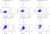 |
Fig. 6. Likelihood distributions for three mock datasets between the two intrinsic parameters describing the flexible dust attenuation recipes (see text). The 2D and 1D likelihood distributions are represented in each panel for the Calzetti-like recipe (upper panels, parameters δ (x axis, powerlaw_slope) and E(B − V)star/E(B − V)line (y axis, E_BV_factor)) and for the DBPL-free recipe (lower panels, parameters n ISM (x axis, slope_ISM) and μ (y axis, mu)). The contour plots correspond to 68, 95 and 99% of the 2D likelihood distributions. The redshifts of the three selected sources are chosen to be representative of the whole sample: from left to right z = 0.7, 1 and 1.3. The blue vertical and horizontal lines represent the true input values. The labels on the plots are the output parameter names defined in CIGALE. |
Another potential issue is the presence of a UV bump in the attenuation curve which may affect the determination of dust absorption parameters and in particular the slope of the attenuation curve. It is possible to introduce a UV bump in the Calzettilike module and such a prescription was already used in various studies (Buat et al. 2012; Kriek & Conroy 2013; Zeimann et al. 2015). We perform a run with a bump of free amplitude. A positive value of the amplitude is returned for most objects with an average value corresponding to ~40% of the value found for the MW extinction curve. With at most one broad-band filter overlapping the UV bump, its detection is not safe and we can only say that we do not exclude the presence of a bump. The impact on the measure of when the bump is considered is a very slight average increase of its values by 0.04±0.09. It never exceeds 0.2 except for two objects for which the difference is of the order of 0.3. For these two SEDs the u band filter overlaps the UV bump and an amplitude for the bump as large as the one of the MW extinction curve is returned by the fit, while there is no valid NUV flux to constrain the slope of the attenuation curve at shorter wavelengths. Such a configuration (positive bump from the fit and no valid NUV data) is realized only for these two objects. As expected the impact of the presence of the UV bump on the estimation of E(B − V)star/E(B − V)line is less important with an average difference between the value obtained with and without the bump of −0.02 ± 0.06. We therefore conclude that the measurement of the dust attenuation parameters introduced in the flexible recipes is robust.
Both parameters μ and E(B − V)star/E(B − V)line measure the differential attenuation affecting young and old stars with a slightly different definition as explained in Sect. 3.3. In the upper panel of Fig. 7, μ and E(B − V)star/E(B − V)line are both found in general higher than the values originally adopted by Charlot & Fall (2000) and Calzetti et al. (2000) (0.3 and 0.44 respectively). They have a correlation coefficient of 0.72. Although the two quantities are both related to differential attenuation between young and old stellar populations, we do not expect a 1:1 relation since their definition as well as the separation between young and old stars are different. In the case of Calzetti-like recipe the nebular and stellar emission are considered separately, only very young and massive stars contribute efficiently to the nebular emission reddened with E(B − V)line when E(B − V)star refers to the attenuation of the continuum emission produce by the stellar population as a whole. The DBPL-free method splits the stellar population in a young and old component whose attenuation is different and μ is defined as  which is the ratio of the attenuation applied to the old and young stars. Using similar quantities, μ can be compared to
  7: these two quantities are found to strongly correlate (R = 0.83) with a mean ratio of
  .
.
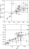 |
Fig. 7. Comparison of the parameters of the attenuation laws. Upper panel: factor of differential attenuation, μ (x axis) against E(B − V)star/E(B − V)line (y axis) for the recipes DBPL-free and Calzetti-like respectively. Lower panel: slopes of the attenuation laws, power-law exponent n ISM for DBPL-free (x axis) against δ for Calzetti-like (y axis). In both panels the values of the original recipes C00 and CF00 are indicated with dashed lines. |
The exponent n ISM of the DBPL-free recipe is also found to correlate with δ, which modifies the C00 law, with a correlation coefficient of 0.74 (lower panel of Fig. 7). The values of δ are found lower than 0 for all but two galaxies and only 8 galaxies are fitted with an average n ISM < −0.7. While the value δ of is sufficient to get the effective attenuation curve to apply to the stellar population with our Calzetti-like model, the shape of the effective attenuation curve resulting from the DBPL-free model depends not only on n ISM but also on μ and on the SFH since young and old populations are attenuated in different ways. In order to easily compare the relative variation of the attenuation laws with wavelength obtained with both recipes, we calculate the total attenuation in the FUV, V and H band filters (with central wavelength 0.15, 0.55 and 1.6 μm respectively) in order to study the UV to visible and visible to NIR regimes.
In Fig. 8 the ratios of the attenuation in FUV and V, and H and V respectively are compared. It can be seen that the Calzettilike recipe returns a steeper curve (i.e. a higher A FUV/AV and a lower AH/AV ). The difference is much stronger in the visible to NIR: AH/AV is found similar for all the sources fitted with the Calzetti-like recipe: adding a powerlaw dependence does not change the shape of the law in the visible to NIR as already shown by Lo Faro et al. (2017). The DBPL-free attenuation laws are always flatter than the Calzetti-like laws in the visible to NIR and, as expected, become grayer (AH/AV increasing) as n ISM increases.
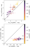 |
Fig. 8. Upper panel: comparison of values obtained for A FUV/AV with the flexible recipes for dust attenuation DPBL-free (x axis) and Calzettilike (y axis). The power-law exponent of the attenuation law in the ISM for the DBPL-free recipe is color coded. Lower panel: same with AH/AV . |
We illustrate the dependence of the DBPL-free attenuation law on μ by plotting the variation of A FUV/AV with n ISM and μ for our best models in Fig. 9, a clear trend is seen with an increase of A FUV/AV when μ decreases, for a given n ISM. We expect a large impact of the differential attenuation on the effective attenuation curve in the UV to visible range (e.g., Inoue 2005). When μ = 1, all the stars are obscured with the same attenuation law which is a single power-law of exponent n ISM. As μ decreases, the young stars emitting at lower wavelengths than the older ones are more attenuated: the attenuation law becomes steeper and A FUV/AV increases. The SFH also plays a role as shown in Charlot & Fall (2000), in the present case our galaxies experiment similar SFHs (no strong burst, delayed star formation rate). Nevertheless, an effect of the recent star formation activity can be seen in Fig. 9 where A FUV/AV does not have a strictly monotonic variation with μ.
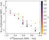 |
Fig. 9. Ratio of the attenuation in the FUV and V bands as a function of n ISM for the recipe DBPL-free. The ratio of the V band attenuation experimented by old and young stars, μ, is color coded. The parameters of the best models are used instead of the means of the PDFs, in order to get clear trends between them |
4.3. Recovering the Hα emission
In Fig. 10 the observed 3D-HST Hα fluxes are plotted against the flux deduced from the fits for the four attenuation scenarios. A very good agreement is found for the sources detected in Hα with a signal to noise ratio higher than 2. As expected the dispersion of the correlation between the observed and estimated fluxes is lower with flexible attenuation recipes. The three galaxies marginally detected in Hα with a signal to noise ratio lower than 2 are represented in red in Fig. 10. Accounting for the uncertainty of the observed Hα flux, the observed and fitted fluxes are consistent within 1σ.
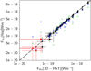 |
Fig. 10. Comparison of observed 3D-HST Hα fluxes (x axis) with Hα fluxes estimated from the fits (y axis). The 4 attenuation recipes are considered: DBPL-free (filled squares), Calzetti-like (filled circles), CF00 (blue empty squares), C00 (green empty circles). The sources detected in Hα with a signal to noise ratio lower than 2 are represented in red with the same symbols as mentioned before. The dashed line is the 1:1 relation. The 1σ uncertainty on both measurements (observation and fit) is reported for only two flexible recipes (DPBL-free and Calzetti-like) to make the plot more clear. |
The attenuations in Hα obtained with the two scenarios are compared in Fig. 11, a good agreement is found for the galaxies detected in Hα with a signal to noise ratio larger than 2. The average value of A Hα , is found to be 2.35 ± 0.75 and 2.00 ± 0.68 mag for the DBPL-free and Calzetti-like recipes respectively. It is around twice the usual value found for nearby Hα selected galaxies (Garn & Best 2010). One of the three sources with a S/N < 2 in Hα is not represented in Fig. 11: it exhibits very discrepant A Hα , the DBPL-free modeling gives a Hα attenuation of 9.2 ± 5.7 mag against 3.7 ± 0.1 mag with the Calzetti-like model. Despite this large discrepancy, the low impact of the Hα flux in the fits (due to its large error) as well as the absence of very young stars (no recent burst) makes the other measurements like the SFR or the attenuation in the FUV or the V band consistent.
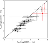 |
Fig. 11. Comparison of Hα attenuations obtained with the recipes DBPL-free (x axis) and Calzetti-like (y axis). The 1σ uncertainty on both measurements is reported. The two sources represented in red are detected in H with an S/N < 2, a third source also detected with an S/N < 2 is not represented (see text). |
5. Discussion
5.1. Average attenuation properties
Our fitting method with flexible attenuation recipes allows us to estimate simultaneously the shape of the attenuation laws and the amount of attenuation for each emission component defined in the recipe adopted for the fit. Moreover, the IR data strongly constrain the measure of the attenuation through the energy balance. Previous studies measured either the differential attenuation (Kashino et al. 2013; Price et al. 2014; Puglisi et al. 2016) or only fit the shape of the attenuation law (Salmon et al. 2016; Salim et al. 2018). The analyses based on spectroscopy, both for the continuum and the emission lines, are able to measure all the characteristics of the attenuation process, with methods similar to that of Calzetti et al. (1994) (Reddy et al. 2015; Battisti et al. 2016). However a robust absolute calibration of the law should be based on the IR emission from dust reemission as performed by Calzetti et al. (2000).
The average values of slope, differential attenuation, and absolute values of V band and Hα attenuations found for our sample of galaxies are given in Table 2. The average slope corresponding to the Calzetti-like recipe is close to the average value found by Buat et al. (2012) for a sample of galaxies selected in UV and observed in IR, and steeper than the original law of C00. DBPL-free gives slighter flatter slopes than Calzetti-like modeling (cf. Fig. 8) and the average value is consistent within 1σ with the original value of CF00. The difference between the average slopes of our two flexible recipes is explained by the introduction of substantial visible to NIR attenuation with DBPL-free which leads to less attenuation in the FUV. The consistency with the CF00 power-law exponent explains why the fits are only slightly improved when n ISM is taken free (Sect. 4 and Fig. 2), it also justifies to use the CF00 value of −0.7 for the entire HELP datasets.
Average characteristics of the attenuation laws with the recipes DBPL-free and Calzetti-like.
5.2. Comparison with previous measurements
The comparison of our results to the ones already published is possible with the Calzetti-like modeling adopted in several studies, where most of the authors also compare their results to the original C00 law. Kriek & Conroy (2013) built composite SEDs including Hα features and derived UV slopes (δ parameter) and UV bump from their fits. They found that δ is increasing with the Hα equivalent width. Our sample spans a moderate range of Hα equivalent widths, from 10 to 40 Å, with a median value of 13 Å and our average value of δ is fully consistent with their measurements. At higher redshift, Zeimann et al. (2015) also used the Calzetti-like formalism, they found no evidence of a UV bump and shallow attenuation laws (δ > 0.2) for galaxies with stellar masses lower than ~1010 M ⊙. Salmon et al. (2016) also found that most of their galaxies have steeper slopes than the C00 law. However the average relation they found between the color excess and δ (their Fig. 9) leads to a value of δ close to 0 for our average attenuation (AV = 1.36 ± 0.48 mag with the Calzetti-like recipe). Slopes as steep as ours correspond to lower color excess (~0.1 mag). Lo Faro et al. (2017) used the DBPL-free recipes to fit ULIRGs and found very flat attenuation curves for these galaxies which experience a strong attenuation with an average AV of 2.5 mag, in agreement with a flattening of the attenuation curve when the attenuation increases (Salmon et al. 2016).
The average ratio of the color excess for the stellar and nebular emission is consistent within 1σ with the 0.44 value valid of nearby starbursting galaxies. The ratio, μ, of the V-band attenuations for old and young stars has an average value twice the original value proposed by CF00. Several studies at different redshifts, all assuming a C00 law also found values consistent with or close to 0.44 (Garn et al. 2010; Price et al. 2014; Mancini et al. 2011; Wuyts et al. 2011) whereas other ones (Kashino et al. 2013; Puglisi et al. 2016) found more similar attenuations for nebular and stellar emission. The comparison between these studies is difficult since most of them apply the C00 law to both emissions. If absolute attenuations are measured from comparisons of SFRs (Garn et al. 2010; Mancini et al. 2011; Wuyts et al. 2011) the original value of C00 corresponding E(B−V)star/E(B−V)line must be translated from 0.44 to 0.57 (e.g., Pannella et al. 2015). The direct measurements of color excesses with Balmer decrement and SED fitting are not affected by this issue (Kashino et al. 2013; Price et al. 2014). The sample used by Puglisi et al. (2016) is also built from 3D-HST and Herschel data and could be considered close to our selection although they have PACS data for only half of their sample. They found that a value of 0.93, higher than 0.57, has to be used to make consistent the SFR deduced from the UV, IR, Hα data. In addition to a different sample selection, the analyses also differ with a comparison of SFR based on standard recipes versus SED fitting with a large number of parameters. Puglisi et al. (2016) use the C00 law for their comparison when we also fit the shape of the attenuation curve. The variation of the attenuation curve is not considered in any of the works mentioned above. When we compare the values of E(B − V)star/E(B − V)line obtained with our C00 and Calzetti-like recipes, the average values are found to be very similar (0.53 against 0.54) but the difference between the two values of E(B − V)star/E(B − V)line can reach 0.2 on individual objects.
Our sample is not well suited to search for correlations between galaxy properties and the parameters of the attenuation law. Its small size and the tight distributions of L IR, M star, SFR or sSFR do not give a sufficient statistics to investigate robust trends. van der Wel et al. (2012) measured structural parameters for galaxies of the CANDELS survey, the Sersic index of our galaxies spans a small range of values from ~0.5 to ~2 and we did not find any significant trend involving this parameter. The axis ratio is better distributed from 0.2 to 0.9 and as expected the attenuation decreases from edge-on to face-on galaxies, although the relation is very dispersed. Anyway, no correlation is found between this axis ratio and the parameters of the attenuation laws.
5.3. Comparison with radiative transfer modeling results
In our analysis we cannot distinguish between the Calzetti-like and DBPL-free modeling, the two scenarios giving fits of similar quality. The consistency of the recipes for the estimation of the shape of the attenuation curve at short wavelengths and the good correlation found between the values of δ and n ISM on one side and μ and E(B − V)star/E(B − V)line on the other side make us confident in the average trends we find. The two recipes return significant differences in the visible to NIR range as already discussed in Lo Faro et al. (2017) who found the DBPL-free recipe to give results more consistent with radiative transfer modeling for dusty ULIRGs. We can also compare our fitting results to the predictions of radiative transfer models. Chevallard et al. (2013) have gathered the results of several radiative transfer models to extract the average predicted slope of the attenuation curve, assumed to be a power-law at λ = 0.55 (nV ) and 1.6 μm (nH ) as a function of the effective attenuation in the corresponding band. To compare with the results of Chevallard et al. (2013) we calculate the slope of our attenuation curves between the FUV band and the V band, then between the V band and the H band. The choice of such a large difference in wavelength to calculate the power law exponents is justified to minimize the uncertainty on their determination and because of the global shapes of the attenuation curves obtained with our recipes. Lo Faro et al. (2017) showed that if the DBPL-free recipe leads to attenuation curves close to a perfect power law it is not the case with the Calzetti-like model and the variation between FUV and V on one side and V and H on the other side give a good global representation of both laws. In Fig. 12, the prediction of the models (Eqs. (9) and (10) of Chevallard et al. 2013) and our resulting slopes are compared. A reasonable agreement is found in the V band for both recipes, our slopes are slighly steeper, especially with the Calzetti-like models. The situation is very different in the NIR: the slopes obtained with the DBPL-free models are in good agreement with the radiative transfer models but the slopes derived with the Calzetti-like recipe are much steeper. The introduction of the δ parameter modifies the slope of the attenuation law in the UV range but has no significant impact on the shape of the attenuation curve in the NIR range while flatter curves are expected from radiative transfer models for the effective attenuation found for our sample galaxies.
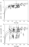 |
Fig. 12. Power-law exponents of the effective attenuation laws measured in the visible (upper panel) and NIR (lower panel) are plotted against the attenuation in the V band, AV . and compared to the mean relations of Chevallard et al. (2013) plotted with a thick line, the thin lines corresponding to the 1σ uncertainty. The values obtained with the DBPL-free and the Calzetti-like modeling are plotted with filled squares and dots respectively. The one σ uncertainties are reported for each quantity. |
6. Conclusion
We have analyzed a complete sample of 34 galaxies at intermediate redshift selected in IR with Herschel PACS and SPIRE detections, with an Hα line detection for each source from the 3D-HST survey. By fitting simultaneously UV to NIR broad band and Hα fluxes we have compared several dust attenuation recipes: the classical Calzetti et al. (2000) and Charlot & Fall (2000) methods and flexible recipes modifying the slope of the effective attenuation curves. The differential attenuation between either stellar and nebular emission or young and old stars was taken as a free parameter for each recipe.
The flexible recipes give the best results with a substantial variation of the slope of the laws and of the differential attenuation, confirming the non-universality of any dust attenuation law. The Charlot & Fall (2000) give satisfactory results in its original form while the slope of the Calzetti et al. (2000) law is substantially modified. The Hα fluxes are very well fitted together with the continuum emission, the mean attenuation in the Hα line is found to be of the order of 2 mag.
The effective attenuation curves obtained with the flexible recipes are found in general steeper than the original ones. Both recipes are consistent with the general trends found with radiative transfer modeling in the visible between the global attenuation and the slope of the effective attenuation law. Large departures are found in the NIR: the flexible recipe based on Charlot & Fall (2000) prescription remains consistent with the results of the models but the multiplication of the Calzetti et al. (2000) law by a power law does not sufficiently flatten the slope of the resulting law in the NIR to reach the values predicted by models.
The attenuation in the V band affecting young stars is found to be, in average, 1.6 times higher than the one found for older stars, a factor 2 lower than the original value proposed by Charlot & Fall (2000), the average value of the ratio between the color excess for stellar continuum and the nebular emission is consistent with the value 0.44 valid for the Calzetti et al. (2000) law. However, both parameters are found to span a large range of values.
We apply the definition adopted by Ciesla et al. (2018): BIC = χ 2 + k × ln(n). χ 2 is the non-reduced of the best fit, k the number of free parameters and n the number of data fitted.


Acknowledgements.
We thank the anonymous referee for her/his very useful comments on validity checks to implement. This study has received funding from the European Union Seventh Framework Programme FP7/2007-2013/ under Grant Agreement Number 60725. MB was supported by the FONDECYT regular project 1170618 and part of the work was done during a stay of VB at Universidad de Antofagasta funded by the FONDECYT project. KM has been also supported by the National Science Centre (grant UMO-2013/09/D/ST9/04030). This work is based on observations taken by the 3D-HST Treasury Program (GO 12177 and 12328) with the NASA-ESA HST, which is operated by the Association of Universities for Research in Astronomy, Inc., under NASA contract NAS5-26555.
References
- Battisti, A. J., Calzetti, D., & Chary, R.-R. 2016, ApJ, 818, 13 [NASA ADS] [CrossRef] [Google Scholar]
- Battisti, A. J., Calzetti, D., & Chary, R.-R. 2017, ApJ, 840, 109 [NASA ADS] [CrossRef] [Google Scholar]
- Boquien, M., Burgarella, D., Roehlly, Y., et al. 2018, A&A, accepted [Google Scholar]
- Boselli, A., Roehlly, Y., Fossati, M., et al. 2016, A&A, 596, A11 [NASA ADS] [CrossRef] [EDP Sciences] [Google Scholar]
- Brammer, G. B., van Dokkum, P. G., Franx, M., et al. 2012, ApJS, 200, 13 [Google Scholar]
- Bruzual, G., & Charlot, S. 2003, MNRAS, 344, 1000 [NASA ADS] [CrossRef] [Google Scholar]
- Buat, V., Giovannoli, E., Heinis, S., et al. 2011, A&A, 533, A93 [NASA ADS] [CrossRef] [EDP Sciences] [Google Scholar]
- Buat, V., Noll, S., Burgarella, D., et al. 2012, A&A, 545, A141 [NASA ADS] [CrossRef] [EDP Sciences] [Google Scholar]
- Calzetti, D. 2001, PASP, 113, 1449 [NASA ADS] [CrossRef] [Google Scholar]
- Calzetti, D., Kinney, A. L., & Storchi-Bergmann, T. 1994, ApJ, 429, 582 [NASA ADS] [CrossRef] [Google Scholar]
- Calzetti, D., Armus, L., Bohlin, R. C., et al. 2000, ApJ, 533, 682 [NASA ADS] [CrossRef] [Google Scholar]
- Cardelli, J. A., Clayton, G. C., & Mathis, J. S. 1989, ApJ, 345, 245 [NASA ADS] [CrossRef] [Google Scholar]
- Casey, C. M., Scoville, N. Z., Sanders, D. B., et al. 2014, ApJ, 796, 95 [NASA ADS] [CrossRef] [Google Scholar]
- Chabrier, G. 2003, PASP, 115, 763 [Google Scholar]
- Charlot, S., & Fall, S. M. 2000, ApJ, 539, 718 [Google Scholar]
- Chevallard, J., & Charlot, S. 2016, MNRAS, 462, 1415 [NASA ADS] [CrossRef] [Google Scholar]
- Chevallard, J., Charlot, S., Wandelt, B., & Wild, V. 2013, MNRAS, 432, 2061 [NASA ADS] [CrossRef] [Google Scholar]
- Ciesla, L., Elbaz, D., Schreiber, C., Daddi, E., & Wang, T. 2018, A&A, 615, A61 [NASA ADS] [CrossRef] [EDP Sciences] [Google Scholar]
- Conroy, C. 2010, MNRAS, 404, 247 [Google Scholar]
- Conroy, C. 2013, ARA&A, 51, 393 [NASA ADS] [CrossRef] [Google Scholar]
- Cullen, F., McLure, R. J., Khochfar, S., et al. 2018, MNRAS, 476, 3218 [NASA ADS] [CrossRef] [Google Scholar]
- da Cunha, E., Charlot, S., & Elbaz, D. 2008, MNRAS, 388, 1595 [Google Scholar]
- Draine, B. T., & Li, A. 2007, ApJ, 657, 810 [NASA ADS] [CrossRef] [Google Scholar]
- Eales, S., Dunne, L., Clements, D., et al. 2010, PASP, 122, 499 [NASA ADS] [CrossRef] [Google Scholar]
- Fossati, M., Mendel, J. T., Boselli, A., et al. 2018, A&A, 614, A57 [NASA ADS] [CrossRef] [EDP Sciences] [Google Scholar]
- Garn, T., & Best, P. N. 2010, MNRAS, 409, 421 [NASA ADS] [CrossRef] [Google Scholar]
- Garn, T., Sobral, D., Best, P. N., et al. 2010, MNRAS, 402, 2017 [NASA ADS] [CrossRef] [Google Scholar]
- Gordon, K. D., Clayton, G. C., Misselt, K. A., et al. 2003, ApJ, 594, 279 [NASA ADS] [CrossRef] [EDP Sciences] [Google Scholar]
- Griffin, M. J., Abergel, A., Abreu, A., et al. 2010, A&A, 518, L3 [Google Scholar]
- Hurley, P. D., Oliver, S., Betancourt, M., et al. 2017, MNRAS, 464, 885 [NASA ADS] [CrossRef] [Google Scholar]
- Inoue, A. K. 2005, MNRAS, 359, 171 [NASA ADS] [CrossRef] [Google Scholar]
- Inoue, A. K. 2011, MNRAS, 415, 2920 [NASA ADS] [CrossRef] [Google Scholar]
- Kashino, D., Silverman, J. D., Rodighiero, G., et al. 2013, ApJ, 777, L8 [NASA ADS] [CrossRef] [Google Scholar]
- Kriek, M., & Conroy, C. 2013, ApJ, 775, L16 [NASA ADS] [CrossRef] [Google Scholar]
- Laigle, C., McCracken, H. J., Ilbert, O., et al. 2016, ApJS, 224, 24 [NASA ADS] [CrossRef] [Google Scholar]
- Lee, S.-K., Ferguson, H. C., Somerville, R. S., Wiklind, T., & Giavalisco, M. 2010, ApJ, 725, 1644 [NASA ADS] [CrossRef] [EDP Sciences] [Google Scholar]
- Lo Faro, B., Buat, V., Roehlly, Y., et al. 2017, MNRAS, 472, 1372 [NASA ADS] [CrossRef] [Google Scholar]
- Malek, K., Buat, V. & Roehlly, Y. et al. 2018, A&A, in press, DOI: 10.1051/0004-6361/201833131 [Google Scholar]
- Mancini, C., Förster Schreiber, N. M., Renzini, A., et al. 2011, ApJ, 743, 86 [NASA ADS] [CrossRef] [Google Scholar]
- Momcheva, I. G., Brammer, G. B., van Dokkum, P. G., et al. 2016, ApJS, 225, 27 [NASA ADS] [CrossRef] [Google Scholar]
- Narayanan, D., Davé, R., Johnson, B. D., et al. 2018, MNRAS, 474, 1718 [NASA ADS] [CrossRef] [Google Scholar]
- Noll, S., Burgarella, D., Giovannoli, E., et al. 2009, A&A, 507, 1793 [NASA ADS] [CrossRef] [EDP Sciences] [Google Scholar]
- Oliver, S. J., Bock, J., Altieri, B., et al. 2012, MNRAS, 424, 1614 [NASA ADS] [CrossRef] [EDP Sciences] [Google Scholar]
- Pacifici, C., Charlot, S., Blaizot, J., & Brinchmann, J. 2012, MNRAS, 421, 2002 [NASA ADS] [CrossRef] [Google Scholar]
- Pacifici, C., da Cunha, E., Charlot, S., et al. 2015, MNRAS, 447, 786 [NASA ADS] [CrossRef] [Google Scholar]
- Pannella, M., Elbaz, D., Daddi, E., et al. 2015, ApJ, 807, 141 [NASA ADS] [CrossRef] [Google Scholar]
- Panuzzo, P., Granato, G. L., Buat, V., et al. 2007, MNRAS, 375, 640 [NASA ADS] [CrossRef] [Google Scholar]
- Pierini, D., Gordon, K. D., Witt, A. N., & Madsen, G. J. 2004, ApJ, 617, 1022 [NASA ADS] [CrossRef] [Google Scholar]
- Pilbratt, G. L., Riedinger, J. R., Passvogel, T., et al. 2010, A&A, 518, L1 [CrossRef] [EDP Sciences] [Google Scholar]
- Poglitsch, A., Waelkens, C., Geis, N., et al. 2010, A&A, 518, L2 [NASA ADS] [CrossRef] [EDP Sciences] [Google Scholar]
- Popping, G., Puglisi, A., & Norman, C. A. 2017, MNRAS, 472, 2315 [NASA ADS] [CrossRef] [Google Scholar]
- Price, S. H., Kriek, M., Brammer, G. B., et al. 2014, ApJ, 788, 86 [NASA ADS] [CrossRef] [Google Scholar]
- Puglisi, A., Rodighiero, G., Franceschini, A., et al. 2016, A&A, 586, A83 [NASA ADS] [CrossRef] [EDP Sciences] [Google Scholar]
- Reddy, N. A., Kriek, M., Shapley, A. E., et al. 2015, ApJ, 806, 259 [NASA ADS] [CrossRef] [Google Scholar]
- Reddy, N. A., Steidel, C. C., Pettini, M., & Bogosavljević, M. 2016, ApJ, 828, 107 [NASA ADS] [CrossRef] [Google Scholar]
- Rodighiero, G., Daddi, E., Baronchelli, I., et al. 2011, ApJ, 739, L40 [NASA ADS] [CrossRef] [Google Scholar]
- Salim, S., Boquien, M., & Lee, J. C. 2018, ApJ, 859, 11 [NASA ADS] [CrossRef] [Google Scholar]
- Salmon, B., Papovich, C., Long, J., et al. 2016, ApJ, 827, 20 [NASA ADS] [CrossRef] [Google Scholar]
- Salpeter, E. E. 1955, ApJ, 121, 161 [Google Scholar]
- Sargent, M. T., Béthermin, M., Daddi, E., & Elbaz, D. 2012, ApJ, 747, L31 [NASA ADS] [CrossRef] [Google Scholar]
- Schreiber, C., Pannella, M., Elbaz, D., et al. 2015, A&A, 575, A74 [NASA ADS] [CrossRef] [EDP Sciences] [Google Scholar]
- Seon, K.-I., & Draine, B. T. 2016, ApJ, 833, 201 [NASA ADS] [CrossRef] [Google Scholar]
- Stanway, E. R., Eldridge, J. J., & Becker, G. D. 2016, MNRAS, 456, 485 [NASA ADS] [CrossRef] [Google Scholar]
- Theios, R. L., Steidel, C. C. & Strom, A. L. et al. 2018, ApJ, submitted [Google Scholar]
- Tuffs, R. J., Popescu, C. C., Völk, H. J., Kylafis, N. D., & Dopita, M. A. 2004, A&A, 419, 821 [NASA ADS] [CrossRef] [EDP Sciences] [Google Scholar]
- van der Wel, A., Bell, E. F., Häussler, B., et al. 2012, ApJS, 203, 24 [NASA ADS] [CrossRef] [Google Scholar]
- van der Wel, A., Franx, M., van Dokkum, P. G., et al. 2014, ApJ, 788, 28 [NASA ADS] [CrossRef] [Google Scholar]
- van Dokkum, P. G., Brammer, G., Fumagalli, M., et al. 2011, ApJ, 743, L15 [NASA ADS] [CrossRef] [Google Scholar]
- Walcher, J., Groves, B., Budavári, T., & Dale, D. 2011, Ap&SS, 331, 1 [NASA ADS] [CrossRef] [Google Scholar]
- Wild, V., Charlot, S., Brinchmann, J., et al. 2011, MNRAS, 417, 1760 [NASA ADS] [CrossRef] [Google Scholar]
- Witt, A. N., & Gordon, K. D. 2000, ApJ, 528, 799 [Google Scholar]
- Wuyts, S., Förster Schreiber, N. M., Lutz, D., et al. 2011, ApJ, 738, 106 [NASA ADS] [CrossRef] [Google Scholar]
- Zeimann, G. R., Ciardullo, R., Gronwall, C., et al. 2015, ApJ, 814, 162 [NASA ADS] [CrossRef] [Google Scholar]
All Tables
Average characteristics of the attenuation laws with the recipes DBPL-free and Calzetti-like.
All Figures
|
Fig. 1. Upper panel: transmission curves of the filters used to build the SED of galaxies, the list of the filters is on the right side of the figure. Lower panel: template SED generated with CIGALE at z = 0.6 and z = 1.6. The solid line is the SED computed with the same modules as the ones used for the fits, with a single model of star formation, dust attenuation and reemission. The red points are the values of the fluxes in the filters whose transmission curves are plotted in the upper panel, the blue squares are mock observations generated by the code with an error of 10% (blue vertical lines, at 3σ). The fluxes are calculated for a total star formation of one solar mass (standard mode for the generation of models with CIGALE). |
| In the text | |
|
Fig. 2. Comparison of the quality of the fits with the four attenuation recipes considered. The best |
| In the text | |
|
Fig. 3. Comparison of SFR and Mstar for the two flexible recipes. The values along the x axis are obtained with the DBPL-free model, the difference between the DBPL-free and Calzetti-like models is plotted on the y axis (DBPL-free minus Calzetti-like logarithmic values). The solid lines are the result of a linear regression. |
| In the text | |
|
Fig. 4. SFR plotted against Mstar for the two flexible recipes DBPL-free (filled squares) and Calzetti-like (dots). The relations of Schreiber et al. (2015) for redshift z = 0.6 and z = 1.6 are represented with solid lines, the redshift of the sources is color coded |
| In the text | |
|
Fig. 5. Distribution of the total attenuation in the V band, for DBPL-free (filled red histogram) and Calzetti-like (blue empty histogram). |
| In the text | |
|
Fig. 6. Likelihood distributions for three mock datasets between the two intrinsic parameters describing the flexible dust attenuation recipes (see text). The 2D and 1D likelihood distributions are represented in each panel for the Calzetti-like recipe (upper panels, parameters δ (x axis, powerlaw_slope) and E(B − V)star/E(B − V)line (y axis, E_BV_factor)) and for the DBPL-free recipe (lower panels, parameters n ISM (x axis, slope_ISM) and μ (y axis, mu)). The contour plots correspond to 68, 95 and 99% of the 2D likelihood distributions. The redshifts of the three selected sources are chosen to be representative of the whole sample: from left to right z = 0.7, 1 and 1.3. The blue vertical and horizontal lines represent the true input values. The labels on the plots are the output parameter names defined in CIGALE. |
| In the text | |
|
Fig. 7. Comparison of the parameters of the attenuation laws. Upper panel: factor of differential attenuation, μ (x axis) against E(B − V)star/E(B − V)line (y axis) for the recipes DBPL-free and Calzetti-like respectively. Lower panel: slopes of the attenuation laws, power-law exponent n ISM for DBPL-free (x axis) against δ for Calzetti-like (y axis). In both panels the values of the original recipes C00 and CF00 are indicated with dashed lines. |
| In the text | |
|
Fig. 8. Upper panel: comparison of values obtained for A FUV/AV with the flexible recipes for dust attenuation DPBL-free (x axis) and Calzettilike (y axis). The power-law exponent of the attenuation law in the ISM for the DBPL-free recipe is color coded. Lower panel: same with AH/AV . |
| In the text | |
|
Fig. 9. Ratio of the attenuation in the FUV and V bands as a function of n ISM for the recipe DBPL-free. The ratio of the V band attenuation experimented by old and young stars, μ, is color coded. The parameters of the best models are used instead of the means of the PDFs, in order to get clear trends between them |
| In the text | |
|
Fig. 10. Comparison of observed 3D-HST Hα fluxes (x axis) with Hα fluxes estimated from the fits (y axis). The 4 attenuation recipes are considered: DBPL-free (filled squares), Calzetti-like (filled circles), CF00 (blue empty squares), C00 (green empty circles). The sources detected in Hα with a signal to noise ratio lower than 2 are represented in red with the same symbols as mentioned before. The dashed line is the 1:1 relation. The 1σ uncertainty on both measurements (observation and fit) is reported for only two flexible recipes (DPBL-free and Calzetti-like) to make the plot more clear. |
| In the text | |
|
Fig. 11. Comparison of Hα attenuations obtained with the recipes DBPL-free (x axis) and Calzetti-like (y axis). The 1σ uncertainty on both measurements is reported. The two sources represented in red are detected in H with an S/N < 2, a third source also detected with an S/N < 2 is not represented (see text). |
| In the text | |
|
Fig. 12. Power-law exponents of the effective attenuation laws measured in the visible (upper panel) and NIR (lower panel) are plotted against the attenuation in the V band, AV . and compared to the mean relations of Chevallard et al. (2013) plotted with a thick line, the thin lines corresponding to the 1σ uncertainty. The values obtained with the DBPL-free and the Calzetti-like modeling are plotted with filled squares and dots respectively. The one σ uncertainties are reported for each quantity. |
| In the text | |
Current usage metrics show cumulative count of Article Views (full-text article views including HTML views, PDF and ePub downloads, according to the available data) and Abstracts Views on Vision4Press platform.
Data correspond to usage on the plateform after 2015. The current usage metrics is available 48-96 hours after online publication and is updated daily on week days.
Initial download of the metrics may take a while.