© ESO 2018

1. Introduction

The past two decades have seen numerous advances in heterodyne radio technologies and their application to modern themes in atmospheric science of planets, small bodies, and astrophysics. These instruments, operating typically in in the submillimetre wave range up to frequencies of 5 THz, provide a very high frequency resolution such that photons from individual rotational transitions of molecules can be measured. These measurements are currently accurate enough with high signal-to-noise ratio such that Doppler shifts in line frequency can be used for wind determination along the line of sight. Perhaps, one of the most important lines is the ortho-water molecule transition (1₁₀ → 1₀₁) at 556.936 GHz, which has become crucial for learning about activities of cold icy objects in the solar system linked to our origins (Bockelee-Morvan 1987; Bensch & Bergin 2004; Zakharov et al. 2007). Several observatories use this transition for detection, for example the Submillimeter Wave Astronomical Satellite (SWAS; Neufeld et al. 2000; Bensch et al. 2007), the Odin satellite equipped with a 1.1 m submillimetre telescope (Biver et al. 2007), and the Heterodyne Instrument for the Far Infrared (HIFI) on the Herschel Space Observatory (Hartogh et al. 2009; de Graauw et al. 2010). Similarly, the analogue transitions of water isotopologues (${\text{H}}_2^{18}\hspace{0.17em}\text{O}$ and HDO) can be used to learn about the origin of water (Hartogh et al. 2011b; Bockelée-Morvan et al. 2012; Biver et al. 2012; Lis et al. 2013). Naturally, molecules other than water can also be easily studied in this wavelength range (HCN, CH₃OH, H₂S, and CS; Biver et al. 2012; de Val-Borro et al. 2012b, 2013).

More recently, the Rosetta mission carried the Microwave Instrument for the Rosetta Orbiter (MIRO; Gulkis et al. 2007) to comet 67P/Churyumov-Gerasimenko, which for more than two years studied the near nucleus coma from rotational transitions of H₂O, NH₃, CO, and CH₃OH (Gulkis et al. 2015; Lee et al. 2015; Biver et al. 2015). Nevertheless, other solar system objects can be studied to detect and monitor the permanent and the transient atmospheres (Lellouch 2008). For instance, we have learned about the tenuous water atmosphere of Ceres from Herschel/HIFI (Küppers et al. 2014), and Saturn’s largest moon Enceladus and its water torus (Hartogh et al. 2011a).

In the future the exploration of the Jovian system as an archetype for gas giants and the characterization of the Ganymede, Europa, Callisto, and Io surface–atmosphere relationship will be taken up by the European JUpiter Icy Moon Explorer (JUICE) mission (Grasset et al. 2013). One of the relevant measurements will be made possible by the Submillimetre Wave Instrument (SWI) to profile the H₂O, winds, and temperature from emission of water lines at 557, 1153, and 1163 GHz in the atmospheres of moons¹.

A well-known difficulty in interpreting these rotational transitions in the tenuous atmosphere of comets, moons, and asteroids stems from the fact that even the rotational populations cannot be assumed to be in local thermodynamic equilibrium (LTE), as noted in all the works cited in the previous paragraph. Furthermore, in the case of the lowest rotational transition of ortho-H₂O a significant optical depth can exist even in such harsh conditions as a cometary coma (Zakharov et al. 2007; Lee et al. 2015). Therefore, accurate non-LTE molecular excitation codes have to be developed. An additional problem for these smaller objects is that their models cannot rely on the plane-parallel assumption typically used for non-LTE in the ro-vibrational bands on the Earth and Mars (López-Puertas & Taylor 2001). The solution of multilevel radiative transfer under non-LTE conditions in spherical symmetry can be considered a classical problem in astrophysics (Kunasz & Hummer 1974a,b; see also Anusha et al. 2009), and it is a demanding computational task even in simple 1D atmospheres. The challenging task is the repeated calculation of the mean radiative field at each atmospheric level required to solve the system of statistical equilibrium equations (SEE; see Sect. 2). A popular technique to simplify the calculation for expanding cometary atmospheres is the so-called escape probability (EP) method (Rybicki 1985; Bockelee-Morvan 1987; Zakharov et al. 2007; de Val-Borro et al. 2012a; O’Rourke et al. 2013). The advantage of EP is that the problem is treated as local (with photon escape probabilities calculated without radiative transfer), and that it is a deterministic method. Another popular method relies on the Monte Carlo (MC) method to obtain the mean intensity (Hogerheijde & Van Der Tak 2000; Zakharov et al. 2007; Lee et al. 2011), which can cope in principle with more complex geometry, but the calculated populations show intrinsic random noise. While both methods show good agreement in the forward simulations of cometary lines Zakharov et al. (2007), the MC method has a clear disadvantage if a routine inverse problem relying on a non-LTE Jacobian matrix has to be solved (Lee et al. 2015).

In this paper we describe the implementation of a state-of-the-art deterministic method for the solution of multilevel non-LTE problem in a 1D spherically symmetric atmosphere able to accurately treat optically thick transitions in both static and expanding atmospheres. The method falls under the class of the Accelerated Lambda Iteration method (ALI; described in the next section), but relies on Gauss–Seidel approach for population corrections during iterations (Trujillo Bueno & Fabiani Bendicho 1995; Asensio Ramos & Trujillo Bueno 2006). The aim is to incorporate the implemented non-LTE model into the public version of the Atmospheric Radiative Transfer Simulator (ARTS; Buehler et al. 2017; Eriksson et al. 2011); the present version is made available via the ARTS-associated python package ‘typhon’.

This paper is set up as follows. Section 2 describes the formalism of radiative transfer in spherical geometry, and the solution of the multilevel non-LTE problem through the concepts of lambda iteration (LI), multilevel ALI (MALI), and multilevel Gauss–Seidel (MUGA). In Sect. 3 we compare the performance of non-LTE methods, and also validate our results under optically thick and thin conditions. Here we also present some forward calculations for the main water transitions in the Ganymede atmosphere predicted by the direct simulations model of Marconi (2007) and an example of additional application of our non-LTE model and spectra calculation in the context of cometary atmospheres as measured by the Rosetta/MIRO instrument. Finally, in Sect. 4 we summarize our main results and provide an outlook for future developments and improvements of the non-LTE model and ARTS.

2. Method of solution non-LTE problem

2.1. Overview

Our main concern is to model radiation intensity associated with rotational transitions of optically active molecules that falls roughly into the submillimetre wave range. Due to a small energy separation between the internal rotational states of molecules, the inelastic collisions within a volume are usually sufficient to keep the rotational populations in Boltzmann distribution, i.e. LTE, for even relatively low densities. In the LTE regime, the population distribution depends uniquely on the kinetic temperature. This is one of the advantages of submillimetre measurements, the possibility to target specific rotational lines typically of the ground vibrational state that are often safely assumed to be in LTE. In contrast, the vibrational populations of a molecule as a result of larger energy spacing among levels depart from LTE at somewhat high densities in atmospheric conditions typical of the Earth (see López-Puertas & Taylor 2001; Feofilov & Kutepov 2012, for discussion of ro-vibrational non-LTE). Nevertheless, in the conditions of cometary comae, icy-moon atmospheres, and at high altitudes in planetary atmospheres the collisions are not usually frequent enough to keep even the rotational level populations according to the Boltzmann distribution and accurate non-LTE modelling needs to be applied.

Generally speaking a non-LTE problem consist of two related parts: (1) the solution of the SEE expressing all the processes populating and de-populating the different levels including radiation and (2) the solution of the radiative transfer equation (RTE) integrated over angle and frequency to produce the mean intensity at each atmospheric level (Kutepov et al. 1998), which in turn depends on level populations.

The most obvious method of solving this interdependent problem is lambda iteration (LI), which repeatedly solves the RTE for the current level populations obtained from the SEE until convergence. However, after many iterations the LI method may often yield an incorrect population distribution, especially in the case of optically thick atmospheres; it is a problem of “false convergence” (Lambert et al. 2015) and for atmospheric science applications see the extensive discussion in Kutepov et al. (1998). In order to compute non-LTE populations for atmospheres with high opacities, an approximate (or accelerated) lambda iteration (ALI) method was devised which was capable of avoiding “trapped” photons in the thick lines, providing accurate and much faster convergence on the populations (Rybicki & Hummer 1991, 1992). An even more effective method (in number of iterations) of computing the non-LTE populations relies on the Gauss–Seidel approach for populations corrections during iteration of the SEE and RTE (Bueno & Sainz 1999; Asensio Ramos & Trujillo Bueno 2006). This method will be discussed in detail in the following section.

In the following section we give a brief overview of the non-LTE solution in spherical symmetry. We have adopted a notation system where each variable that needs to be integrated over the frequency and solid angle have been subindexed with ν and p, respectively. The details of p are described in Sect. 2.2. For variables where lines have to be considered individually, the subindex i j is adopted to indicate a transition from state i to state j. Most of these variables are also dependent on altitude, but we omit this subindex for simplicity until the Gauss–Seidel method description (Sect. 2.4.3), where for the sake clarity the ν sub-index is implicit. Finally, we adapt the bra-ket notations to clearly indicate access to individual elements of the matrices built below.

2.2. Radiative transfer calculations

In this work the solution of the transfer equation is performed on a set of rays tangent to the shells (see Fig. 1). The specific intensity I is computed along rays of constant impact parameter, p (Anusha et al. 2009; Harper 1994). Each ray in Fig. 1 is related to the shell radius and has angles, θ, with intersected shells. These angles are used to integrate specific intensity over directions, Ω, at each altitude, and it is also required for projecting the radial expansion onto the rays to account for the Doppler shift. The number of shells with radius smaller than the planet radius, R, is defined as NC, and the number of the shells larger than R is the same as the number of the given discrete spatial grid m = 1, 2, …, NP. Therefore, the p grid has the length of NC + NP, as shown in Fig. 1. The incoming rays may include a background radiation term and are being propagated until the tangent layer (TH), or until an intersection with the surface, where TH ≤ R. The outgoing parts are continued from the tangent height or started from the surface until the outer layer.

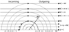Fig. 1. Schematic representation of the placement of ray paths (arrows) of each p for computing the radiation field in spherical geometry. Dotted semicircles represent spherical atmospheric layers at a spatial grid of m − 1, m, m + 1, and NP. The solid semicircle represents a surface of a body where the spatial grid m = 0. Dashed semicircles represent shells inside the surface and dotted straight lines represent the tangent lines to the shells (see text for details).

The macroscopic radiative transfer equation can formally be expressed as

$$\begin{array}{c}\hfill \frac{\mathrm{d}{I}_{\nu }}{\mathrm{d}s}=j_{\nu }-{\alpha }_{\nu }{I}_{\nu },\end{array}$$(1)

where I_ν is the specific intensity [J m⁻² sr⁻¹ Hz⁻¹ s⁻¹] defined as the radiative energy passing through a surface normal to the path per unit time, frequency, and solid angle. The emission coefficient, j_ν, has units of [J m⁻² sr⁻¹ Hz⁻¹ s⁻¹], while the absorption coefficient, α_ν, is in [m⁻¹]. The equation describes the change in I_ν as the radiation travels along a path, where the distance along the path is given by s. In the subsequent description we limit ourselves to photons along a ray due to specific spectral (bound–bound) transitions, and neglect any continuum sources/sinks of radiation and scattering at a given frequency, ν [Hz]. The micro-physical process of emission and absorption can be then expressed as

$$\begin{array}{c}\hfill j_{\nu ,ij}=\frac{h{\nu }_{\mathit{ij}}}{4\pi }{n}_i{A}_{\mathit{ij}}{\varphi }_{\nu }\end{array}$$(2)

and

$$\begin{array}{c}\hfill {\alpha }_{\nu ,ij}=\frac{h{\nu }_{\mathit{ij}}}{4\pi }(n_j{B}_{\mathit{ji}}{\varphi }_{\nu }^{\prime }-n_i{B}_{\mathit{ij}}{\varphi }_{\nu }^{″}),\end{array}$$(3)

where h is the Planck constant, n_i denotes the number density of molecules in an upper level, A_ij is Einstein’s spontaneous emission probability of a transition i → j, and ϕ_ν is the frequency-dependent line emission profile. The local absorption coefficient depends on Einstein’s absorption probability B_ji and Einstein’s stimulated emission probability B_ij. The Einstein coefficients obey the well-known relationship, g_iB_ij = g_jB_ji, where g_i and g_j are the degeneracy at level i and j, respectively, and $A_{ij}=2h{v}_{ij}^3{B}_{ij}{c}^{-2}$. The parameters ϕ′_ν and ϕ″_ν describe the line profiles for absorption and stimulated emission, respectively, and n_j is the number density of molecules in the lower level. Hereafter we rely on the typical assumption of complete angular and frequency redistribution such that the absorption and the emission profiles are approximately equal, ${\varphi }_v={\varphi }_v^{\prime }={\varphi }_v^{″}$.

In the case of macroscopic velocity fields present in the atmosphere, the emission and absorption coefficients incur an angular dependence. Because the angles Ω at a spatial point m vary with the set of rays p, the Doppler shift for a transition i to j at each spatial point m and ray path p is

$$\begin{array}{c}\hfill \mathrm{\Delta }{\nu }_{ij,p}=\frac{-{\upsilon }_p{\nu }_{\mathit{ij}}cos{\theta }_p}{c},\end{array}$$(4)

where υ_p is the radial wind speed and θ_p is the angle between the wind direction at altitude m and line of sight placed at p in Fig. 1 (this is the angle θ as in Fig. 1, with explicit dependence on the ray p).

It is convenient to write the RTE in another more compact form by dividing both sides by α_ν,

$$\begin{array}{c}\hfill \frac{\mathrm{d}{I}_{\nu }}{\mathrm{d}{\tau }_{\nu }}=S-I_{\nu }.\end{array}$$(5)

This notation introduces very useful physical quantities that turn out to be important for understanding the propagation of radiation along a ray. First, the so-called source function, S ≡ j_ν/α_ν, and second, the optical depth, dτ_ν ≡ ∑α_νds, where the sum is performed over all active absorber contributions at the given frequency (non-overlapping lines). There are a number of different solutions to this equation, each with its own strengths, for example the method of short characteristics (SCs; Olson & Kunasz 1987), the Feautrier method (Rybicki & Hummer 1991), and the discontinuous finite element (DFE) method (Castor et al. 1992). In this paper, we only deal with spherically symmetric medium, thus we implemented the very efficient methods of first- and second-order SCs (Olson & Kunasz 1987; see Sect. 2.4.3 and Appendix C for a detailed description).

2.3. Statistical equilibrium

The SEE expresses a balance among all the detailed micro-physical processes influencing the individual population levels. In this paper we assume steady-state conditions such that physical processes influencing the population of levels are much faster than variations in the thermophysical conditions of the atmosphere. In order to calculate the population n_i of each of the i = 1, 2, …, NL levels the code accounts for radiative and collisional processes (with one or more collisional partners), such that at each spatial point we can write

$$\begin{array}{cc}\hfill \frac{\mathrm{d}{n}_i}{\mathrm{d}t}=0=& {\displaystyle \sum _{j>i}[n_j{A}_{\mathit{ji}}-(n_i{B}_{\mathit{ij}}-n_j{B}_{\mathit{ji}}){\overline{J}}_{\mathit{ij}}]}\hfill \\ \hfill & -{\displaystyle \sum _{j<i}[n_i{A}_{\mathit{ij}}-(n_j{B}_{\mathit{ji}}-n_i{B}_{\mathit{ij}}){\overline{J}}_{\mathit{ij}}]}\hfill \\ \hfill & +{\displaystyle \sum _j(n_j{C}_{\mathit{ji}}-n_i{C}_{\mathit{ij}}),}\hfill \end{array}$$(6)

where t is time [s], C_ij [s⁻¹] is the total collisional rate² for transitions from level i to j, and J̄_ij is the integrated mean intensity defined as

$$\begin{array}{c}\hfill {\overline{J}}_{\mathit{ij}}=\frac{1}{4\pi }{\displaystyle {\int }_0^{\infty }\text{d}\nu {\int }_0^{4\pi }\text{d}\mathrm{\Omega }{I}_{\nu }{\varphi }_{ij,\nu }.}\end{array}$$(7)

The line shape function is calculated including the Doppler shift of frequency Eq. (4) in the case of an expanding atmosphere. The first and second term on the right side of Eq. (6) represent the radiative rates between level i and the upper/lower levels, respectively. The third term on the right side of Eq. (6) represents transition rates due to collisional processes.

The resulting system of equations can be formally written as

$$\begin{array}{c}\hfill {\mathbf{A}}^{\prime }·\mathbf{n}=\mathbf{0},\end{array}$$(8)

where A′ is a matrix of size NL × NL whose elements contain the collisional and radiative rates, and n is a vector containing the population of each level. Under the stated assumptions the set of rate equations is singular and requires that one of the rows of the matrix should be replaced with ones, and setting a single value of the right-hand side zero-vector to the total number of molecules. The resulting equation is

$$\begin{array}{c}\hfill \mathbf{A}·\mathbf{n}=\mathbf{f}.\end{array}$$(9)

We note that the diagonal of A (i.e. ⟨i|A|i⟩) represents the sum over the destruction rate coefficient of level i, and ⟨i|A|j⟩ represents the formation rate coefficient from level i to j. As mentioned, one row of A contains ones, and f is a zero-vector, except having the same row replaced by the total number density.

The J̄_ij in Eq. (7) is a non-local function of the emitting and absorbing conditions throughout the medium, and these conditions depend on local values of the populations. Therefore, solving Eq. (9) for the atomic and molecular population distributions is a non-local and, generally, a non-linear problem. The non-LTE multilevel problem consists of finding the populations n satisfying Eq. (9) which use the value of n at each spatial grid to calculate the radiative rates.

2.4. Non-LTE methods

Our non-LTE model adopts the multilevel Gauss–Seidel flavour of the ALI iteration method, which features a very rapid convergence to a true solution (Trujillo Bueno & Fabiani Bendicho 1995). To demonstrate this method’s performance we compare it to two other approaches, namely LI and pure ALI, which are discussed below as precursors to the Gauss–Seidel description.

2.4.1. Lambda iteration method

The LI method uses a simple back-and-forth iteration between the SEE and RTE until convergence is reached. The lambda operator, Λ, acting on a source function is a convenient way to express the calculation of specific intensity, even though it is not implied that such matrix has to be explicitly formed. In this formalism the specific intensity at given altitude can be written as

$$\begin{array}{c}\hfill {\mathbf{I}}_{\nu ,p}={\mathrm{\Lambda }}_{\nu ,p}[\mathbf{S}],\end{array}$$(10)

where S is the source function vector and Λ_{ν, p} is a matrix whose elements ⟨m|Λ_{ν, p}|m′⟩ gives the response of the radiation field at point m due to a unit-perturbation in the source function at point m′ along the line of sight p. Then the integrated mean intensity J̄_ij at each altitude can be written as

$$\begin{array}{c}\hfill {\overline{J}}_{\mathit{ij}}^{\mathrm{old}}=\frac{1}{4\pi }{\displaystyle {\int }_{-\infty }^{\infty }\mathrm{d}\nu {\int }_0^{4\pi }\mathrm{d}\mathrm{\Omega }{\varphi }_{ij,\nu ,p}{\mathrm{\Lambda }}_{\nu ,p}[{\mathbf{S}}^{\mathrm{old}}],}\end{array}$$(11)

where ${\overline{J}}_{\mathit{ij}}^{\mathrm{old}}$ and S^old represent the integrated mean intensity and source function vectors obtained from previous iteration, respectively. The line shape function, ϕ_{ν, p}, is calculated at each set of rays p and altitude grid m.

Once the radiative rates are updated the new level populations are calculated again by solving the linear system,

$$\begin{array}{c}\hfill {\mathbf{A}}^{\mathrm{old}}·{\mathbf{n}}^{\mathrm{new}}=\mathbf{f},\end{array}$$(12)

where n^new is the calculated level populations, and A^old is the A but using integrated mean intensity obtained from the populations calculated by the previous iteration step, n^old. The explicit statistical equilibrium equations (Eq. (6)) for Λ-iteration can be expressed as

$$\begin{array}{cc}& {\displaystyle \sum _{j>i}[n_j^{\mathrm{new}}{A}_{\mathit{ji}}-(n_i^{\mathrm{new}}{B}_{\mathit{ij}}-n_j^{\mathrm{new}}{B}_{\mathit{ji}}){\overline{J}}_{\mathit{ij}}^{\mathrm{old}}]}\hfill \\ \hfill & -{\displaystyle \sum _{j<i}[n_i^{\mathrm{new}}{A}_{\mathit{ij}}-(n_j^{\mathrm{new}}{B}_{\mathit{ji}}-n_i^{\mathrm{new}}{B}_{\mathit{ij}}){\overline{J}}_{\mathit{ij}}^{\mathrm{old}}]}\hfill \\ \hfill & +{\displaystyle \sum _j(n_j^{\mathrm{new}}{C}_{\mathit{ji}}-n_i^{\mathrm{new}}{C}_{\mathit{ij}})=0.}\hfill \end{array}$$(13)

The iteration continues until the conditions for convergence are satisfied. The Λ-iteration is the most direct and simple approach to the problem; however, it is known to be slow to reach convergence for optically thick lines. This occurs because each cycle of the iteration corresponds to photons moving about one mean free path in the medium, hence many iterations are required to move them any substantial distance. Such trapped photons in the cores of optically thick lines provide small updates in the populations (due to radiative field) from one iteration to the next (Rybicki & Hummer 1991; Lambert et al. 2015).

2.4.2. Multilevel accelerated lambda iteration (MALI) method

The multilevel accelerated Λ-iteration, MALI, has much faster convergence rates than Λ-iteration because it effectively removes the trapped photons from consideration through a clever analytical step (e.g. Cannon 1973; Rybicki & Hummer 1991; Auer & Paletou 1994).

In ALI, we write the full Λ-operator as ${\mathrm{\Lambda }}_{\nu ,p}={\mathrm{\Lambda }}_{\nu ,p}^{\ast }+({\mathrm{\Lambda }}_{\nu ,p}-{\mathrm{\Lambda }}_{\nu ,p}^{\ast })$, where ${\mathrm{\Lambda }}_{\nu ,p}^{\ast }$ is the approximate (local) version of the Λ-operator. Substituting this expression into the formula for specific intensity (10), we obtain

$$\begin{array}{c}\hfill {\mathbf{I}}_{\nu ,p}\simeq {\mathrm{\Lambda }}_{\nu ,p}^{\ast }\left[{\mathbf{S}}^{\mathrm{new}}\right]+({\mathrm{\Lambda }}_{\nu ,p}-{\mathrm{\Lambda }}_{\nu ,p}^{\ast })\left[{\mathbf{S}}^{\mathrm{old}}\right],\end{array}$$(14)

where S^old and S^new represent the source function vectors obtained from the previous iteration and current iteration, respectively. From Eqs. (7), (11), and (14), the integrated mean intensity at each spatial point is written as

$$\begin{array}{c}\hfill {\overline{J}}_{\mathit{ij}}\simeq {\overline{J}}_{\mathit{ij}}^{\mathrm{old}}+{\overline{\mathrm{\Lambda }}}_{\mathit{ij}}^{\ast }(S_{\mathit{ij}}^{\mathrm{new}}-S_{\mathit{ij}}^{\mathrm{old}}),\end{array}$$(15)

where ${\overline{J}}_{\mathit{ij}}^{\mathrm{old}}$ is the integrated mean intensity obtained from the population calculated by previous iteration step. The parameter ${\overline{\mathrm{\Lambda }}}_{\mathit{ij}}^{\ast }$ is integral over frequency and direction of ⟨m|Λ_{ν, p}|m⟩ for a transition between i and j at spatial point at m:

$$\begin{array}{c}\hfill {\overline{\mathrm{\Lambda }}}_{\mathit{ij}}^{\ast }=\frac{1}{4\pi }{\displaystyle {\int }_{-\infty }^{\infty }\mathrm{d}\nu {\int }_0^{4\pi }\mathrm{d}\mathrm{\Omega }{\varphi }_{ij,\nu ,p}⟨m|{\mathrm{\Lambda }}_{\nu ,p}|m⟩.}\end{array}$$(16)

Because S^new in Eq. (15) is

$$\begin{array}{c}\hfill S_{\mathit{ij}}^{\mathrm{new}}=\frac{n_i^{\mathrm{new}}{A}_{\mathit{ij}}}{n_j^{\mathrm{new}}{B}_{\mathit{ji}}-n_i^{\mathrm{new}}{B}_{\mathit{ij}}},\end{array}$$(17)

we can express SEE at each spatial point including the approximate radiative transfer effect as follows:

$$\begin{array}{cc}& {\displaystyle \sum _{j>i}[n_j^{\mathrm{new}}{A}_{\mathit{ji}}(1-{\overline{\mathrm{\Lambda }}}_{\mathit{ij}}^{\ast })-(n_i^{\mathrm{new}}{B}_{\mathit{ij}}-n_j^{\mathrm{new}}{B}_{\mathit{ji}})({\overline{J}}_{\mathit{ij}}^{\mathrm{old}}-{\overline{\mathrm{\Lambda }}}_{\mathit{ij}}^{\ast }{S}_{\mathit{ij}}^{\mathrm{old}})]}\hfill \\ \hfill & -{\displaystyle \sum _{j<i}[n_i^{\mathrm{new}}{A}_{\mathit{ij}}(1-{\overline{\mathrm{\Lambda }}}_{\mathit{ij}}^{\ast })-(n_j^{\mathrm{new}}{B}_{\mathit{ji}}-n_i^{\mathrm{new}}{B}_{\mathit{ij}})({\overline{J}}_{\mathit{ij}}^{\mathrm{old}}-{\overline{\mathrm{\Lambda }}}_{\mathit{ij}}^{\ast }{S}_{\mathit{ij}}^{\mathrm{old}})]}\hfill \\ \hfill & +{\displaystyle \sum _j(n_j^{\mathrm{new}}{C}_{\mathit{ji}}-n_i^{\mathrm{new}}{C}_{\mathit{ij}})=0.}\hfill \end{array}$$(18)

The terms $(1-{\overline{\mathrm{\Lambda }}}_{\mathit{ij}}^{\ast })$ and $({\overline{J}}_{\mathit{ij}}^{\mathrm{old}}-{\overline{\mathrm{\Lambda }}}_{\mathit{ij}}^{\ast }{S}_{\mathit{ij}}^{\mathrm{old}})$ in the radiative rates in Eq. (18) are pre-conditioning the system, and remain linear in populations. We should also note that when the problem converges, Eqs. (14), (15), and (18) become exact as ${\overline{\mathrm{\Lambda }}}_{\mathit{ij}}^{\ast }$ goes to 0. The resulting linear system of equation is

$$\begin{array}{c}\hfill {\mathbf{A}}_{\mathrm{MALI}}^{\mathrm{old}}·{\mathbf{n}}^{\mathrm{new}}=\mathbf{f},\end{array}$$(19)

and the iteration proceeds basically in the same was as in the Λ-iteration, the difference being the pre-conditioning of the radiative rates.

2.4.3. Multilevel Gauss–Seidel (MUGA) method

The Gauss–Seidel iterative method based on the idea of solving the Eq. (9) sequentially from the lowermost (uppermost) layer toward the uppermost (lowermost) layer by updating the current source function value and performing full angular integration of the specific intensity by using new level populations. This method was first presented by Trujillo Bueno & Fabiani Bendicho (1995), and Fabiani Bendicho et al. (1997) gives a suitable summary of its application to the multilevel problem in Cartesian coordinates. The first implementation of this method in spherical symmetry for problems in astrophysical applications are given in Asensio Ramos & Trujillo Bueno (2006).

As we set out to solve the system of Eq. (19) the mean intensity at each iteration step, J̄_{m,i j} can be corrected by calculating the radiation field with new level populations at the spatial point of m − 1. To update J̄_{m,i j} at spatial point m we separate the specific intensity into outward-directed intensity (I_{m, p↑}) and inward-directed intensity (I_{m, p↓}), expressing them as

$$\begin{array}{cc}\hfill I_{m,p\uparrow }=I_{m-1,p\uparrow }exp(-\mathrm{\Delta }{\tau }_{m-\frac{1}{2},p})+& {\displaystyle {\int }_{m-1}^m{S}_{m^{\prime }}\exp (-{\tau }_{m,p}+{\tau }_{m^{\prime },p})\text{d}{m}^{\prime }}\hfill \end{array}$$(20)

and

$$\begin{array}{cc}\hfill I_{m,p\downarrow }=I_{m+1,p\downarrow }exp(-\mathrm{\Delta }{\tau }_{m+\frac{1}{2},p})& +{\displaystyle {\int }_m^{m+1}{S}_{m^{\prime }}exp(-{\tau }_{m,p}+{\tau }_{m^{\prime },p})\text{d}{m}^{\prime },}\hfill \end{array}$$(21)

where

$$\begin{array}{c}\hfill \mathrm{\Delta }{\tau }_{m\pm \frac{1}{2},p}=|{\tau }_{m,p}-{\tau }_{m\pm 1,p}|.\end{array}$$(22)

These outward- and inward-directed intensities, except for the bottom and top layers, can be updated when Eqs. (20) and (21) are discretized by the second-order short characteristics method (Olson & Kunasz 1987). The second-order method interpolates the source function by a parabola going through S_{m − 1}, S_m, S_{m + 1} using the Lagrangian interpolation,

$$\begin{array}{cc}\hfill I_{m,p\uparrow }^{\mathrm{new}}=& I_{m-1,p\uparrow }^{\mathrm{new}}exp(-\mathrm{\Delta }{\tau }_{m-\frac{1}{2},p}^{\mathrm{new}})\hfill \\ \hfill & +{\lambda }_{m-1,p\uparrow }^{\mathrm{new}}{S}_{m-1}^{\mathrm{new}}+{\lambda }_{m,p\uparrow }^{\mathrm{new}}{S}_m^{\mathrm{old}}+{\lambda }_{m+1,p\uparrow }^{\mathrm{new}}{S}_{m+1}^{\mathrm{old}}\hfill \end{array}$$(23)

and

$$\begin{array}{cc}\hfill I_{m,p\downarrow }^{\mathrm{new}}=& I_{m+1,p\downarrow }^{\mathrm{old}}exp(-\mathrm{\Delta }{\tau }_{m+\frac{1}{2},p})\hfill \\ \hfill & +{\lambda }_{m+1,p\downarrow }^{\mathrm{new}}{S}_{m+1}^{\mathrm{old}}+{\lambda }_{m,p\downarrow }^{\mathrm{new}}{S}_m^{\mathrm{old}}+{\lambda }_{m-1,p\downarrow }^{\mathrm{new}}{S}_{m-1}^{\mathrm{new}},\hfill \end{array}$$(24)

where the each term with superscript “new” indicates that it is calculated by using new level populations in iteration steps. The details of how to calculate the interpolation coefficients, λ, in Eqs. (23) and (24) are detailed in Appendix C. As described in Olson & Kunasz (1987), the ${\overline{\mathrm{\Lambda }}}_{m,ij}^{\ast }$ for spatial point m is

$$\begin{array}{c}\hfill {\overline{\mathrm{\Lambda }}}_{m,ij}^{\ast }=\frac{1}{4\pi }{\displaystyle {\int }_{\infty }^{\infty }\mathrm{d}\nu {\int }_0^{4\pi }\mathrm{d}\mathrm{\Omega }{\varphi }_{ij,m,p}[{\lambda }_{m,p\uparrow }+{\lambda }_{m-1,p\uparrow }exp(-\mathrm{\Delta }{\tau }_{m-\frac{1}{2},p\uparrow })}\\ \hfill +{\lambda }_{m,p\downarrow }+{\lambda }_{m+1,p\downarrow }exp(-\mathrm{\Delta }{\tau }_{m+\frac{1}{2},p\downarrow })].\end{array}$$(25)

Then by using the corrected ${\overline{\mathrm{\Lambda }}}_{m,ij}^{\ast }$ and integrated mean intensity, ${\overline{J}}_{m,i,j}^{\mathrm{old}\&\mathrm{new}}$, the statistical equilibrium equation can be written as

$$\begin{array}{cc}& {\displaystyle \sum _{j>i}[n_{m,j}^{\mathrm{new}}{A}_{\mathit{ji}}(1-{\overline{\mathrm{\Lambda }}}_{m,ij}^{\ast })}\hfill \\ \hfill & -(n_{m,i}^{\mathrm{new}}{B}_{\mathit{ij}}-n_{m,j}^{\mathrm{new}}{B}_{\mathit{ji}})({\overline{J}}_{m,ij}^{\mathrm{old}\&\mathrm{new}}-{\overline{\mathrm{\Lambda }}}_{m,ij}^{\ast }{S}_{m,ij}^{\mathrm{old}})]\hfill \\ \hfill & -{\displaystyle \sum _{j<i}[n_{m,i}^{\mathrm{new}}{A}_{\mathit{ij}}(1-{\overline{\mathrm{\Lambda }}}_{m,ij}^{\ast })}\hfill \\ \hfill & -(n_{m,j}^{\mathrm{new}}{B}_{\mathit{ji}}-n_{m,i}^{\mathrm{new}}{B}_{\mathit{ij}})({\overline{J}}_{m,ij}^{\mathrm{old}\&\mathrm{new}}-{\overline{\mathrm{\Lambda }}}_{m,ij}^{\ast }{S}_{m,ij}^{\mathrm{old}})]\hfill \\ \hfill & +{\displaystyle \sum _j(n_{m,j}^{\mathrm{new}}{C}_{m,ji}-n_{m,i}^{\mathrm{new}}{C}_{m,ij})=0.}\hfill \end{array}$$(26)

The expression ${\overline{J}}_{m,i,j}^{\mathrm{old}\&\mathrm{new}}$ at spatial grid m is the integrated mean intensity obtained by Eq. (7). The resulting linearized system of the equation at every altitude point is

$$\begin{array}{c}\hfill {\mathbf{A}}_{\mathrm{GS}}^{\mathrm{old}\&\mathrm{new}}·{\mathbf{n}}_{\mathrm{new}}=\mathbf{f},\end{array}$$(27)

where ${\mathbf{A}}_{\mathrm{GS}}^{\mathrm{old}\&\mathrm{new}}$ indicates using the corrected mean intensity calculated by radiative transfer taking account of perturbation of the population correction at each spatial grid.

As mentioned in Asensio Ramos & Trujillo Bueno (2006), it is important to clarify that the multilevel Gauss–Seidel method requires a specific order of the loops over transitions, angles (direction of the radiation), and spatial points when propagating the radiation. The most external loop is the one over directions, first going inwards and then outwards. The next is the loop over spatial points, followed by the loop over transitions. The most internal ones are the loops over angles and frequencies. The reason is that we need to evaluate the mean intensity for all the radiative transitions in order to be able to perform the population correction before advancing to the following point of the spatial grid.

3. Validation of the MUGA non-LTE method implementation

In this section we describe the validation and performance of our implementation of the non-LTE solver based on the MUGA method (Asensio Ramos & Trujillo Bueno 2006). This is accomplished by comparing calculated populations to other existing non-LTE models for similar applications. In this validation we use a MALI code implementation for rotational level populations, as used in Rezac et al. (2013; hereafter MPS-ALI), and served as a benchmark for implementing the EP method used for cometary observations (Marshall et al. 2017). In addition, we also use the widely applied and freely available Monte Carlo non-LTE code RATRAN³, described in the paper Hogerheijde & Van Der Tak (2000).

3.1. Input data and computational details

The most frequent and scientifically important observations in the submillimetre wave range from space telescopes target the low-lying rotational transitions of water. For this purpose we work with the ortho-H₂O non-LTE model typically used in cometary applications (Bensch & Bergin 2004; Hartogh et al. 2011b; Lee et al. 2015). This model considers seven ortho-H₂O levels with nine transitions (see Fig. 2). We use the LAMDA⁴ molecular database (Schöier et al. 2005) for level energies, degeneracies, frequencies, and spontaneous emission rates for each transition (see Appendix D).

The collisional coefficient data, and their temperature dependences were obtained from Buffa et al. (2000). In this paper we only consider H₂O–H₂O collisions (i.e. single collisional partner). In future work, when absolute accuracy for the scientific investigations with a proper non-LTE model for Ganymede’s spectral line measurements may be required, additional collision partners shall be considered.

In this validation we first consider a static water atmosphere of Ganymede as simulated by a kinetic model described in Marconi (2007). We consider optically thick and optically thin conditions to test our implementation, which are represented as subsolar latitude (SSL) 10° and 60°, respectively. The associated temperature and number density profiles are shown in Fig. 3.

The extent of the atmosphere is taken up to 450 km from the surface. Above this altitude the water number density becomes too low to significantly contribute to relevant measurements (except perhaps near the subsolar point), but other physical effects not considered in our model may also start to play a significant role in the excitation. Another assumption is that the molecular velocity distribution is Maxwellian, which may not always be the case in reality if the source of water molecules is sputtering (Marconi 2007; Turc et al. 2014). The vertical profiles of number density and temperature are discretized into 100 layers. The frequency grid of each transition extends to plus and minus five times that of the full width at half maximum of the Doppler broadening at the highest temperature. In the presented calculations we distribute frequency steps in such a way that there are 200 grid points for each transition line. The numerical integration in Eq. (7) relies on the trapezoidal rule. Nonetheless, these topics are not of importance for demonstrating the performance of our code implementation.

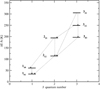Fig. 2. Energy level diagram of the ortho-H2O molecule showing all the levels considered in this work, shown along with all the transitions. This is complementary to the information in Table D.2.

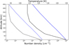Fig. 3. Vertical profiles of temperature (black lines) and number density (blue lines) of Ganymede atmosphere at subsolar latitude 10° (solid lines) and 60° (dashed lines) obtained from the kinetic model of Ganymede’s atmosphere (Marconi 2007).

In the calculations, we assume an equilibrium between the first atmospheric layer and the surface temperature as the lower boundary condition, for convenience. Based on our initial sensitivity tests, we ignore additional external sources such as solar radiance or cosmic background radiation in these examples. Therefore, the upper boundary condition has no incoming radiation field. When discussing convergence performance of the different approaches we refer to the percent difference changes in the populations between successive iterations,

$$\begin{array}{c}\hfill max\left|\frac{{\mathbf{n}}^{\text{new}}-{\mathbf{n}}^{\text{old}}}{{\mathbf{n}}^{\text{old}}}\right|\times 100<0.1.\end{array}$$(28)

The iterations proceed until the relative change of populations on each level and each spatial point reach 0.1% for all the test cases.

Finally, the level populations calculated by the different codes are compared in terms of excitation temperature, T_ex, defined for each transition as

$$\begin{array}{c}\hfill T_{\mathrm{ex}}=-h{\nu }_{\mathit{ij}}/kln\frac{n_i{g}_j}{n_j{g}_i}.\end{array}$$(29)

The T_ex provide an intuitive understanding where in the atmosphere the LTE/non-LTE transitions occurs and whether the excitation is sub- or superthermal. Nevertheless, T_ex only denotes a relative degree of excitation and does not directly translate into spectral emission intensity, which depends on the total number of excited molecules in the given state.

3.2. Results: populations comparison

The profiles of T_ex for the optically thick case, SSL 10°, are plotted in Fig. 4.

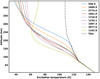Fig. 4. Vertical profiles of excitation temperatures of the nine transitions calculated for the atmospheric model corresponding to SSL = 10°. The labels displayed in the upper right corner denote the frequency for the given transition in GHz. The 556.9 GHz is typically one of the most important transitions for cometary and planetary contexts discussed in this text. The kinetic temperature profile is also shown as dash-dotted line.

In this case the populations start to depart from LTE at around 100 km, while the strong 557 GHz transition is kept thermalized to an altitude above 150 km. In the non-LTE region all the excitation temperatures are noticeably lower than kinetic (subthermal), which is understood as a result of the spontaneous emission rate being greater than the collisional rate, and the absorption of upwelling radiation cannot compensate for the emission process. Although we do not run this model with the solar radiation pumping we have estimated that this effect would be negligible in these examples. A more complex issue is the excitation of the 557 GHz transition from the ground up to ≈180 km, where the upper level of this transition is populated strongly due to spontaneous decay (2₂₁ → 1₁₀), which leads to a value of T_ex slightly higher than the kinetic temperature. For this transition the thermalization process is purely radiative due to opacity effects (exchange of radiation among atmospheric layers) up to 180 km where it cannot compete with the spontaneous emission.

In the optically thin case, the excitation temperatures depart from LTE from the ground as demonstrated in Fig. 5. The collisional frequency is too low to thermalize the levels, and the opacity is too low for radiative exchange among layers to play any role. It is only the upwelling radiation which contributes to a degree to excitation in the near-ground altitudes. The combination of optically weak medium and a low kinetic temperature, specifically the 1162 GHz line has an excitation temperature higher than kinetic above ∼100 km. Nevertheless, even in the weak line limit, i.e. J̄_{i j} = 0, this line’s T_ex is around 100 K at 100 km altitude in this case.

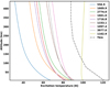Fig. 5. Vertical profiles of excitation temperatures of the nine transitions calculated for the atmospheric model corresponding to SSL = 60°. The labels displayed in the upper right corner denote the frequency for the given transition in GHz. The kinetic temperature profile is also shown as dash-dotted line.

Figures 6 and 7 show the absolute differences between MUGA, MPS-ALI, and RATRAN calculations in terms of T_ex for the two Ganymede atmospheric cases.

Overall, in the optically thick case the codes provide very consistent vertical profiles of the populations. The maximum differences of 0.5 K are reached around a narrow altitude region of 200 km for the 557 GHz transition with respect to the MPS-ALI code (the left panel in Fig. 6), but agree almost perfectly at other altitudes. For the higher lying transitions the MUGA code obtains about 0.5–1 K higher excitation temperatures above 100 km altitude. The largest deviation is just below 1.5 K for the 1162 GHz transition between the highest energy levels considered in this model. The likely explanation for these discrepancies lies in the radiative transfer calculations of the mean intensity that strongly shape the population distribution in this case. This conclusion is further supported by the results in the optically thin scenarios presented below. The comparisons with RATRAN also shows a very good agreement, although there appears to be a semi-constant offset (cold bias in RATRAN calculations) of roughly 1.6 K as shown in the right panel in Fig. 6. We should note that RATRAN is not designed specifically to handle lower boundary conditions, so we artificially imposed in the first 100 m of the atmosphere an infinite optical thickness. The code then treats this implicitly as a surface. Nevertheless, if we were to adjust the offset the absolute differences in value would not exceed ∼2 K. Another obvious and expected feature of the RATRAN calculations is the random scatter of the T_ex on the order of 0.5 K, as we set up this run with a high signal-to-noise ratio. The signal-to-noise ratio and initial number of photons per cell for the RATRAN calculations were 50 and 10000, respectively. This is typically not a problem (for spectral line simulation) if only forward calculations are required, and shows that RATRAN, with slight modification, can be applied to such cases.

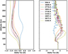Fig. 6. Left panel: profiles of absolute difference of the excitation temperatures calculated in this work (MUGA) and the MPS-ALI code and right panel: the same, but compared against calculations made by the RATRAN package. The atmospheric inputs correspond to the SSL = 10° conditions (see Fig. 4 for Tex magnitude). Lines of different colours correspond to the transitions as shown in the label in units of GHz.

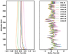Fig. 7. As in Fig. 6, but for atmospheric conditions of SSL = 60° (optically thin case; see Fig. 5 for Tex magnitude).

The optically thin example (Fig. 7) demonstrates that MUGA, MPS-ALI, and RATRAN generally provide the same altitude profiles of populations with differences smaller than 1 K, typically less than 0.5 K. We note that larger deviations between MUGA and MPS-ALI are below 50 km; this is where the lower boundary emissions have the greatest influence on the populations. Above that, the very optically thin conditions mean that the radiative transfer plays no role, and we do not see any vertical structure in the T_ex, as was the case for the optically thick scenario. This indicates that the MUGA and MPS-ALI have small differences in handling the mean intensity calculations and layer-to-layer radiative transfer. The RATRAN calculations are performed in the same manner as described above, with the first 100 m of atmosphere acting as an artificial surface to get the lower boundary condition effects. Judging from the right panel in Fig. 7, a small but constant negative bias remains (perhaps 0.5 K), although the random noise has increased to about 1 K. This is a well-known feature of Monte Carlo radiative transfer codes, it is difficult to build statistics for layers which are more than 99% transparent to the photons. Nevertheless, even in the optically thin conditions the comparisons show a good agreement among the codes.

The MUGA implementation appears to provide accurate populations, and here we discuss its superiority in terms of how many iterations are required to reach subsequent population changes of less than 0.1%. We choose a realistic case and show the maximum change in populations versus iterations for the optically thick scenario of Ganymede atmosphere presented previously. The Fig. 8 contrasts the convergence evolution for MUGA, MALI, and LI methods.

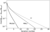Fig. 8. Convergence plots by different iteration methods, MUGA (solid line), MALI (dashed line), and LI (dotted line), for the seven-level H2O model of Ganymede’s atmosphere at SSL = 10o . The vertical axis shows the maximum values of the relative difference between populations at each iteration step and the population which solved the system.

This figure only demonstrates the well-known fact that MUGA provides about a factor of 2 faster convergence compared to MALI. In this example, which is not extremely optically thick, the MUGA provides only a factor 3 improvement over LI. However, this is not a constant factor (as in MALI) since for even larger optical depths the LI method could fail to converge altogether due to the trapped photons (see similar plots and discussion in Bueno & Sainz 1999; Asensio Ramos & Trujillo Bueno 2006; Paletou & Léger 2007). The computation time for solving the non-LTE problem depends linearly on the number of spatial grid points in atmosphere (NP), the number of frequency points, the number of rays (NC+NP), and the number of iterations as described in Asensio Ramos & Trujillo Bueno (2006).

3.3. Results: spectral line simulations with ARTS

In this section we demonstrate the working interface between the non-LTE code, implemented in the python package “typhon”, used to calculate the level populations for a set of input data and ARTS, the general code for outgoing spectra synthesis. In the following examples we use ARTS to calculate synthetic pencil beam spectra for nadir and limb geometries for Ganymede’s atmospheres at the 557 GHz water transition, most often used for detection in the submillimetre wavelengths. As was demonstrated in Sect. 3.2, the populations depart from LTE even in the relatively high density region near the subsolar point. Therefore, to show the importance of taking into account these effects we use both LTE and non-LTE line simulations (Fig. 9) in the Rayleigh–Jeans (RJ) brightness temperature. The receiver is placed at 500 km.

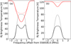Fig. 9. Pencil beam simulated spectra of H2O(110 − 101) for limb (black lines) and nadir (red lines) geometries for Ganymede’s atmosphere with different SSL, 10° (panel a) and 60° (panel b). The receiver was positioned just outside the atmosphere at 500 km. The tangent heights of the line of sight for the limb geometries are 250 km and 50 km altitudes for SSL 10° and 60°, respectively. Dashed lines represent the LTE simulated spectra and solid lines represent the simulated spectra including the non-LTE model.

It is evident that in both geometries the non-LTE effects are pronounced. The LTE/non-LTE differences are consistent with the excitation temperatures shown in Figs. 4 and 5. The subthermal excitation yields non-LTE limb emissions weaker than LTE, while absorption lines are deeper than for the LTE case, as more molecules are in the ground state.

Finally, we demonstrate that the presented MUGA non-LTE code solver in combination with ARTS spectra simulator can be already applied to real measurements. For this purpose we take the submillimetre observations of cometary (67P/Churyumov-Gerasimenko) spectra obtained by the MIRO instruments on board the Rosetta spacecraft. The instrument and early science results with the measurements are presented in Gulkis et al. (2007) and Gulkis et al. (2015), respectively. The aim here is not to derive any scientific results, conclusions, or parameters of interest from the measurement, but rather to demonstrate the applicability of the code. Therefore, we selected an ad hoc sample calibrated spectrum of the ortho-water at 557 GHz from the MIRO database⁵, corresponding to the beginning of “near-nucleus” observations. There are two reasons for the choice of this period: (1) an adequate parametrized model for the temperature, density, and velocity fields have already been published (Lee et al. 2015) and (2) the coma density for this period is just large enough to provide a moderately optical thickness, but too small to completely saturate the line, which would require a much more detailed coma model.

The MIRO measured spectra taken at 2014-08-08T03:58:32 in nadir geometry is shown in Fig. 10. The spacecraft altitude was 82 km from the comet centre at this time. To increase the signal-to-noise ratio we averaged a total of ten minutes of observations, as in Lee et al. (2015), such that the time stamp above indicates the centre time.

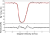Fig. 10. Top panel: comparison of the measurement (black line) and forward model (red line) spectra for the ortho-H2O (557 GHz) transition in nadir geometry (see text for details). Bottom panel: residual between the simulation and measurement spectra.

The simulated MIRO spectra rely on the same seven-level non-LTE model as described for our Ganymede simulations, which is the same as used by Lee et al. (2015). The five parameters needed for the coma model (see Table 1 in Lee et al. 2015) were estimated manually by comparing the measured and simulated spectra until a satisfactory fit was found. The physical parameters are production rate, Q, and terminal expansion velocity, ν₀. The other two coefficients are used in a power law for temperature and another in hyperbolic-tangent function for velocity. The original paper provides retrieved values for Q and ν₀. Our estimate for the sample spectra yields a production rate (≈Q = 2 × 10²⁶ sec⁻¹) and ν₀ = 0.66 km s⁻¹, which is consistent with the overall results of Lee et al. (2015). We did not perform an inverse problem to find the optimal parameters, which is beyond the scope of this work, and fitting other observations (with large optical depth) may even require a more complex coma model beyond the five parameters (Lee et al. 2015). Nevertheless, we demonstrate for a suitable set of molecular and atmospheric inputs the new implemented MUGA code for rotational transitions coupled with ARTS can be used as an effective tool for scientific investigations of relevant measurements in non-LTE conditions.

4. Conclusions

We presented an implementation of an accurate and efficient numerical method of the solution for the non-LTE problem in spherical symmetry. This non-LTE code is aimed at applications where populations of pure rotational transitions of a given vibrational level are required, for example interpretation of submillimetre observations of cometary comae or icy moon atmospheres.

The adopted non-LTE method relies on the state-of-the-art approach developed in the context of stellar astrophysics, the so called Gauss–Seidel ALI method (Trujillo Bueno & Fabiani Bendicho 1995; Asensio Ramos & Trujillo Bueno 2006). This method has two advantages: it is deterministic, so that there is no random scatter in populations typical of Monte Carlo based RT solvers such as RATRAN, and b) it explicitly treats the RT among atmospheric layers, not relying on the simplifying assumption needed, for example, in the escape probability approach. The MUGA method also features a very rapid convergence to the solution, nearly a factor of two improvement relative to the popular ALI method for optically thick conditions. In addition, the ALI and MUGA approaches avoid the problem of extremely slow convergence which ultimately leads to an incorrect solution typical of the pure LI approach in optically thick media.

The non-LTE package is implemented in the Python language, with the goal of making this code a part of the ARTS radiative transfer package. The present communication with ARTS is via its Python interface, the equally open-sourced typhon. ARTS uses the relative level populations passed via this interface to calculate emission and absorption coefficients⁶ for spectra calculation in any available geometry accounting for beam convolution if required in the simulation. The presented non-LTE code⁷ is available under MIT license and ARTS⁸ is available via GPL license.

In order to verify and validate our implementation of the MUGA method we compared the calculated non-LTE populations under optically thin and thick conditions in the context of Ganymede’s water atmosphere against other codes routinely applied to the non-LTE conditions of comets and other astrophysical sources, such as the RATRAN and ALI codes (Rezac et al. 2013; Marshall et al. 2017). Ganymede’s atmosphere is assumed to be static (no expansion velocity). Under the optically thick conditions we demonstrate very good agreements between the available codes; expressed as excitation temperatures for each transition, the differences are below 0.5 K for the main H₂O line (557 GHz) and below 1.5 K for any of the nine lines applied in this non-LTE model. For the optically thin conditions the non-LTE calculations become sensitive to the lower boundary conditions; however, even here the codes show very good agreement, T_ex less than 1 K for all transitions at all altitudes. The RATRAN 1D Monte Carlo approach shows a little larger discrepancy (random noise and small offset); however, we acknowledge that it is not designed explicitly to treat this kind of application, with static atmosphere with important contribution from the surface boundary condition. Nevertheless, it still compares well with the MUGA/ALI results modelling the Ganymede non-LTE atmosphere.

The spectra calculations performed by the ARTS package relying on the interface to the typhon package non-LTE calculations of vertical profile of populations are also presented. The nadir and limb observational geometries were compared, and showed very good agreement in the LTE tests case and also for the full non-LTE calculations. We have also applied the typhon and ARTS codes to simulations of expanding cometary atmospheres under moderately optically thick conditions, and compared them to the nadir measured line profile at 557 GHz obtained by the MIRO/Rosetta instrument. The coma atmosphere was estimated using the parametrized profiles described in Lee et al. (2015).

The new non-LTE package makes a great addition to the ARTS radiative transfer package already established and adapted in many application in atmospheric and planetary science. We demonstrate the accuracy and efficiency of the non-LTE method for the common examples of atmospheres where they are observable. Although we focus only on H₂O transitions in this work, any other molecule can be treated since the simulations are fully determined by the atmospheric, spectroscopic, molecular, and collisional data inputs. In the future, the non-LTE package can be further improved, for example to treat line overlapping in the case of hyper-fine lines. In the near future, we will also implement the contribution of solar radiation in the excitation of the rotational populations via so called g-factors, as described in the work of Zakharov et al. (2007). The future applications of this code can be both the synthetic simulations of future missions (JUICE) or an existing dataset on cometary comas (MIRO).

Acknowledgments

We acknowledge the Principal Investigator M. Hofstadter (NASA/JPL, Pasadena, USA) and the ESA Planetary Science Archive for making available the MIRO data used in this paper. The spectroscopic and collisional data for the non-LTE simulations of ortho-water are freely available from the LAMDA database (http://home.strw.leidenuniv.nl/~moldata/). The calibrated MIRO spectra (2014-08-08T03:58:32) used in this work are also available from the ESA archive (ftp://psa.esac.esa.int/pub/mirror/INTERNATIONAL-ROSETTA-MISSION/MIRO/). The atmospheric profiles have been extracted from the paper of Marconi (2007) and are available from the author upon request.

References

Appendix A: A note on the ARTS implementation

The main calculations of state level distributions are performed outside of the main ARTS program, in a module of its accompanying python package: typhon. In ARTS absorption can be treated for a myriad of species and types of absorption from line-by-line absorption to collision-induced absorption, and various types of empirical/analytical continua. In addition, scattering is considered, adding to complications at even the most fundamental level of how to define the radiative transfer equation.

To fit within this wider theoretical framework, while not being detrimental to the speed of the algorithm in general, the main difference between the internal formalism in this work and the practical implementation in the ARTS code is that j_ν is computed indirectly as a relative ratio while being summed up. That is, for a single absorption line we have

$$\begin{array}{c}\hfill j_{\nu }=B_{\nu }(T_{\mathrm{kin}})({\alpha }_{\nu }+j_{\nu }^{\prime }),\end{array}$$(A.1)

where

$$\begin{array}{c}\hfill j_{\nu }^{\prime }\stackrel{\mathrm{def}}{=}\frac{j_{\nu }}{B_{\nu }(T_{\mathrm{kin}})}-{\alpha }_{\nu }.\end{array}$$(A.2)

While this might appear to be a great slowdown and cumbersome workaround, it allows us to add scattering absorption to α_ν of Eq. (A.1) without changing the treatment of the individual line in Eq. (A.2). It also means that we do not need to touch j_ν for overlapping lines or for cases where we can treat some absorption lines with LTE formalism. The latter is not expected for rotational non-LTE, but can happen when vibrational non-LTE matters.

Appendix B: LTE populations where collisional processes dominate the transitions

The collisional rate, C_ij, described in Eq. (6) is equal to

$$\begin{array}{c}\hfill C_{\mathit{ul}}=n_{\mathrm{col}}{\gamma }_{\mathit{ul}},\end{array}$$(B.1)

where n_col is the number density of the collision partner (in cm⁻³) and γ_ul is the downward collisional rate coefficient (in cm³ s⁻¹), usually temperature dependent. In the case of multiple collisional partners the individual collisional rates are summed up.

The rate coefficient is the Maxwellian average of the collision cross section, σ,

$$\begin{array}{c}\hfill {\gamma }_{\mathit{ul}}={\left(\frac{8k{T}_{\mathrm{kin}}}{\pi \mu }\right)}^{-1/2}{\left(\frac{1}{k{T}_{\mathrm{kin}}}\right)}^2\int \sigma Eexp(-E/k{T}_{\mathrm{kin}})dE,\end{array}$$(B.2)

where E is the collision energy, k is the Boltzmann constant, and μ is the reduced mass of the system. The upward rate is obtained through detailed balance

$$\begin{array}{c}\hfill {\gamma }_{\mathit{lu}}={\gamma }_{\mathit{ul}}\frac{g_u}{g_l}exp\left(\frac{-h{\nu }_{\mathit{ul}}}{k{T}_{\mathrm{kin}}}\right).\end{array}$$(B.3)

Therefore, the population ratio when the thermal collisional processes dominate the transitions can be easily derived as

$$\begin{array}{c}\hfill \frac{n_u}{n_l}=\frac{C_{\mathit{lu}}}{C_{\mathit{ul}}}=\frac{g_u}{g_l}exp\left(\frac{-h{\nu }_{\mathit{ul}}}{k{T}_{\mathrm{kin}}}\right).\end{array}$$(B.4) Kutepov et al. (1998) nicely explain the population in the TE and LTE state. Because the rate constant of γ is related to the Lorentz half-widths, Δν_L, of the transition (see Pack 1979),

$$\begin{array}{c}\hfill \mathrm{\Delta }{\nu }_{\mathrm{L}}={\alpha }_{\mathrm{L}}\frac{p}{p_0}{\left(\frac{T_0}{T}\right)}^n=\frac{1}{2\pi c}\frac{p}{\mathit{kT}}{\gamma }_{\mathit{ul}},\end{array}$$(B.5)

the rate constant of γ_ul can be described as

$$\begin{array}{c}\hfill {\gamma }_{\mathit{ul}}={\alpha }_{\mathrm{L}}\frac{2\pi ckT}{p_0}{\left(\frac{T_0}{T}\right)}^n,\end{array}$$(B.6)

where α_L is the Lorentz half-width at the reference temperature T₀ and reference pressure p₀, p is air pressure, and c is the speed of light. This approach was used by Kutepov et al. (1997) for their study of rotational non-LTE for CO.

Appendix C: Computation definitions of λ in Eqs. (23) and (24) in first- and second-order SC methods

The λ parameters in the Eq. (23) are calculated by

$$\begin{array}{cc}& {\lambda }_{m-1,p\uparrow }\stackrel{\mathrm{def}}{=}{\omega }_0+\frac{{\omega }_2-{\omega }_1(\mathrm{\Delta }{\tau }_{m+\frac{1}{2},p}+2\mathrm{\Delta }{\tau }_{m-\frac{1}{2},p})}{\mathrm{\Delta }{\tau }_{m-\frac{1}{2},p}(\mathrm{\Delta }{\tau }_{m-\frac{1}{2},p}+\mathrm{\Delta }{\tau }_{m+\frac{1}{2},p})},\hfill \end{array}$$(C.1a)

$$\begin{array}{cc}& {\lambda }_{m,p\uparrow }\stackrel{\mathrm{def}}{=}\frac{{\omega }_1(\mathrm{\Delta }{\tau }_{m-\frac{1}{2},p}-\mathrm{\Delta }{\tau }_{m+\frac{1}{2},p})-{\omega }_2}{\mathrm{\Delta }{\tau }_{m-\frac{1}{2},p}\mathrm{\Delta }{\tau }_{m+\frac{1}{2},p}},\hfill \end{array}$$(C.1b)

$$\begin{array}{cc}& {\lambda }_{m+1,p\uparrow }\stackrel{\mathrm{def}}{=}\frac{{\omega }_2-{\omega }_1\mathrm{\Delta }{\tau }_{m-\frac{1}{2},p}}{\mathrm{\Delta }{\tau }_{m+\frac{1}{2},p}(\mathrm{\Delta }{\tau }_{m-\frac{1}{2},p}+\mathrm{\Delta }{\tau }_{m+\frac{1}{2},p})},\hfill \end{array}$$(C.1c)

$$\begin{array}{cc}& {\omega }_0\stackrel{\mathrm{def}}{=}1-exp(-\mathrm{\Delta }{\tau }_{m-\frac{1}{2},p}),\hfill \end{array}$$(C.1d)

$$\begin{array}{cc}& {\omega }_1\stackrel{\mathrm{def}}{=}{\omega }_0-\mathrm{\Delta }{\tau }_{m-\frac{1}{2},p}exp(-\mathrm{\Delta }{\tau }_{m-\frac{1}{2},p}),\hfill \end{array}$$(C.1e)

$$\begin{array}{cc}& {\omega }_2\stackrel{\mathrm{def}}{=}2{\omega }_1-\mathrm{\Delta }{\tau }_{m-\frac{1}{2},p}^{2}exp(-\mathrm{\Delta }{\tau }_{m-\frac{1}{2},p}),\hfill \end{array}$$(C.1f)

for second-order SC, and for Eq. (24)

$$\begin{array}{cc}& {\lambda }_{m+1,p\downarrow }\stackrel{\mathrm{def}}{=}{\omega }_0+\frac{{\omega }_2-{\omega }_1(\mathrm{\Delta }{\tau }_{m-\frac{1}{2},p}+2\mathrm{\Delta }{\tau }_{m+\frac{1}{2},p})}{\mathrm{\Delta }{\tau }_{m+\frac{1}{2},p}(\mathrm{\Delta }{\tau }_{m+\frac{1}{2},p}+\mathrm{\Delta }{\tau }_{m-\frac{1}{2},p})},\hfill \end{array}$$(C.2a)

$$\begin{array}{cc}& {\lambda }_{m,p\downarrow }\stackrel{\mathrm{def}}{=}\frac{{\omega }_1(\mathrm{\Delta }{\tau }_{m+\frac{1}{2},p}-\mathrm{\Delta }{\tau }_{m-\frac{1}{2},p})-{\omega }_2}{\mathrm{\Delta }{\tau }_{m+\frac{1}{2},p}\mathrm{\Delta }{\tau }_{m-\frac{1}{2},p}},\hfill \end{array}$$(C.2b)

$$\begin{array}{cc}& {\lambda }_{m-1,p\downarrow }\stackrel{\mathrm{def}}{=}\frac{{\omega }_2-{\omega }_1\mathrm{\Delta }{\tau }_{m+\frac{1}{2},p}}{\mathrm{\Delta }{\tau }_{m-\frac{1}{2},p}(\mathrm{\Delta }{\tau }_{m+\frac{1}{2},p}+\mathrm{\Delta }{\tau }_{m-\frac{1}{2},p})},\hfill \end{array}$$(C.2c)

$$\begin{array}{cc}& {\omega }_0\stackrel{\mathrm{def}}{=}1-exp(-\mathrm{\Delta }{\tau }_{m+\frac{1}{2},p}),\hfill \end{array}$$(C.2d)

$$\begin{array}{cc}& {\omega }_1\stackrel{\mathrm{def}}{=}{\omega }_0-\mathrm{\Delta }{\tau }_{m+\frac{1}{2},p}exp(-\mathrm{\Delta }{\tau }_{m+\frac{1}{2},p}),\hfill \end{array}$$(C.2e)

$$\begin{array}{cc}& {\omega }_2\stackrel{\mathrm{def}}{=}2{\omega }_1-\mathrm{\Delta }{\tau }_{m+\frac{1}{2},p}^{2}exp(-\mathrm{\Delta }{\tau }_{m+\frac{1}{2},p}).\hfill \end{array}$$(C.2f)

The intensities for any angle at the bottom and top atmospheric layer is calculated by first-order short characteristic method. The first order SC formula of Eqs. (C.1) are simplified to

$$\begin{array}{cc}& {\lambda }_{m-1,p\uparrow }\stackrel{\mathrm{def}}{=}{\omega }_0-\frac{{\omega }_1}{\mathrm{\Delta }{\tau }_{m-\frac{1}{2},p}},\hfill \end{array}$$(C.3a)

$$\begin{array}{cc}& {\lambda }_{m,p+}\stackrel{\mathrm{def}}{=}\frac{{\omega }_1}{\mathrm{\Delta }{\tau }_{m-\frac{1}{2},p}},\hfill \end{array}$$(C.3b)

$$\begin{array}{cc}& {\lambda }_{m+1,p+}\stackrel{\mathrm{def}}{=}0,\hfill \end{array}$$(C.3c)

$$\begin{array}{cc}& {\omega }_0\stackrel{\mathrm{def}}{=}1-exp(-\mathrm{\Delta }{\tau }_{m-\frac{1}{2},p}),\hfill \end{array}$$(C.3d)

$$\begin{array}{cc}& {\omega }_1\stackrel{\mathrm{def}}{=}{\omega }_0-\mathrm{\Delta }{\tau }_{m-\frac{1}{2},p}exp(-\mathrm{\Delta }{\tau }_{m-\frac{1}{2},p}),\hfill \end{array}$$(C.3e)

and Eqs. (C.2) are simplified to

$$\begin{array}{cc}& {\lambda }_{m+1,p\downarrow }\stackrel{\mathrm{def}}{=}{\omega }_0-\frac{{\omega }_1}{\mathrm{\Delta }{\tau }_{m+\frac{1}{2},p}},\hfill \end{array}$$(C.4a)

$$\begin{array}{cc}& {\lambda }_{m,p}\stackrel{\mathrm{def}}{=}\frac{{\omega }_1}{\mathrm{\Delta }{\tau }_{m+\frac{1}{2},p}},\hfill \end{array}$$(C.4b)

$$\begin{array}{cc}& {\lambda }_{m-1,p}\stackrel{\mathrm{def}}{=}0,\hfill \end{array}$$(C.4c)

$$\begin{array}{cc}& {\omega }_0\stackrel{\mathrm{def}}{=}1-exp(-\mathrm{\Delta }{\tau }_{m+\frac{1}{2},p}),\hfill \end{array}$$(C.4d)

$$\begin{array}{cc}& {\omega }_1\stackrel{\mathrm{def}}{=}{\omega }_0-\mathrm{\Delta }{\tau }_{m+\frac{1}{2},p}exp(-\mathrm{\Delta }{\tau }_{m+\frac{1}{2},p}).\hfill \end{array}$$(C.4e)

Appendix D: Input data of molecular parameters in this study

Table D.1 shows the level energies and degeneracies at each level of ortho-H₂O rotational state we considered in this study. Table D.2 shows frequencies and spontaneous emission coefficients for each transition in this study.

All Tables

All Figures

Fig. 1. Schematic representation of the placement of ray paths (arrows) of each p for computing the radiation field in spherical geometry. Dotted semicircles represent spherical atmospheric layers at a spatial grid of m − 1, m, m + 1, and NP. The solid semicircle represents a surface of a body where the spatial grid m = 0. Dashed semicircles represent shells inside the surface and dotted straight lines represent the tangent lines to the shells (see text for details).

In the text

	Fig. 2. Energy level diagram of the ortho-H2O molecule showing all the levels considered in this work, shown along with all the transitions. This is complementary to the information in Table D.2.
In the text

	Fig. 3. Vertical profiles of temperature (black lines) and number density (blue lines) of Ganymede atmosphere at subsolar latitude 10° (solid lines) and 60° (dashed lines) obtained from the kinetic model of Ganymede’s atmosphere (Marconi 2007).
In the text

Fig. 4. Vertical profiles of excitation temperatures of the nine transitions calculated for the atmospheric model corresponding to SSL = 10°. The labels displayed in the upper right corner denote the frequency for the given transition in GHz. The 556.9 GHz is typically one of the most important transitions for cometary and planetary contexts discussed in this text. The kinetic temperature profile is also shown as dash-dotted line.

In the text

	Fig. 5. Vertical profiles of excitation temperatures of the nine transitions calculated for the atmospheric model corresponding to SSL = 60°. The labels displayed in the upper right corner denote the frequency for the given transition in GHz. The kinetic temperature profile is also shown as dash-dotted line.
In the text

Fig. 6. Left panel: profiles of absolute difference of the excitation temperatures calculated in this work (MUGA) and the MPS-ALI code and right panel: the same, but compared against calculations made by the RATRAN package. The atmospheric inputs correspond to the SSL = 10° conditions (see Fig. 4 for Tex magnitude). Lines of different colours correspond to the transitions as shown in the label in units of GHz.

In the text

	Fig. 7. As in Fig. 6, but for atmospheric conditions of SSL = 60° (optically thin case; see Fig. 5 for Tex magnitude).
In the text

	Fig. 8. Convergence plots by different iteration methods, MUGA (solid line), MALI (dashed line), and LI (dotted line), for the seven-level H2O model of Ganymede’s atmosphere at SSL = 10o . The vertical axis shows the maximum values of the relative difference between populations at each iteration step and the population which solved the system.
In the text

Fig. 9. Pencil beam simulated spectra of H2O(110 − 101) for limb (black lines) and nadir (red lines) geometries for Ganymede’s atmosphere with different SSL, 10° (panel a) and 60° (panel b). The receiver was positioned just outside the atmosphere at 500 km. The tangent heights of the line of sight for the limb geometries are 250 km and 50 km altitudes for SSL 10° and 60°, respectively. Dashed lines represent the LTE simulated spectra and solid lines represent the simulated spectra including the non-LTE model.

In the text

	Fig. 10. Top panel: comparison of the measurement (black line) and forward model (red line) spectra for the ortho-H2O (557 GHz) transition in nadir geometry (see text for details). Bottom panel: residual between the simulation and measurement spectra.
In the text

References

- Anusha, L. S., Nagendra, K. N., Paletou, F., & Léger, L. 2009, ApJ, 704, 661 [NASA ADS] [CrossRef] [Google Scholar]
- Asensio Ramos, A., & Trujillo Bueno, J. 2006, EAS Pub. Ser., 18, 25 [CrossRef] [Google Scholar]
- Auer, L. H., & Paletou, F. 1994, A&A, 284, 675 [NASA ADS] [Google Scholar]
- Bensch, F., & Bergin, E. A. 2004, ApJ, 615, 531 [NASA ADS] [CrossRef] [Google Scholar]
- Bensch, F., Melnick, G. J., Neufeld, D. A., et al. 2007, Icarus, 191, 267 [CrossRef] [Google Scholar]
- Biver, N., Bockelée-Morvan, D., Crovisier, J., et al. 2007, Planet. Space Sci., 55, 1058 [NASA ADS] [CrossRef] [Google Scholar]
- Biver, N., Crovisier, J., Bockelée-Morvan, D., et al. 2012, A&A, 539, A68 [NASA ADS] [CrossRef] [EDP Sciences] [Google Scholar]
- Biver, N., Hofstadter, M., Gulkis, S., et al. 2015, A&A, 583, A3 [NASA ADS] [CrossRef] [EDP Sciences] [Google Scholar]
- Bockelee-Morvan, D. 1987, A&A, 181, 169 [NASA ADS] [Google Scholar]
- Bockelée-Morvan, D., Biver, N., Swinyard, B., et al. 2012, A&A, 544, L15 [NASA ADS] [CrossRef] [EDP Sciences] [Google Scholar]
- Buehler, S. A., Mendrok, J., & Eriksson, P. 2017, Geoscientific Model Development Discussions, 1, 436 [Google Scholar]
- Bueno, J. T., & Sainz, R. M. 1999, ApJ, 1, 436 [NASA ADS] [CrossRef] [Google Scholar]
- Buffa, G., Tarrini, O., Scappini, F., & Cecchi-Pestellini, C. 2000, ApJS, 128, 597 [NASA ADS] [CrossRef] [Google Scholar]
- Cannon, C. J. 1973, ApJ, 185, 621 [NASA ADS] [CrossRef] [Google Scholar]
- Castor, J. I., Dykema, P. G., & Klein, R. I. 1992, ApJ, 387, 561 [NASA ADS] [CrossRef] [Google Scholar]
- de Graauw, T., Helmich, F. P., Phillips, T. G., et al. 2010, A&A, 518, L6 [NASA ADS] [CrossRef] [EDP Sciences] [Google Scholar]
- de Val-Borro, M., Hartogh, P., Jarchow, C., et al. 2012a, A&A, 545, A2 [NASA ADS] [CrossRef] [EDP Sciences] [Google Scholar]
- de Val-Borro, M., Rezac, L., Hartogh, P., et al. 2012b, A&A, 546, L4 [NASA ADS] [CrossRef] [EDP Sciences] [Google Scholar]
- de Val-Borro, M., Küppers, M., Hartogh, P., et al. 2013, A&A, 559, A48 [NASA ADS] [CrossRef] [EDP Sciences] [Google Scholar]
- Eriksson, P., Buehler, S., Davis, C., Emde, C., & Lemke, O. 2011, J. Quant. Spectr. Rad. Transf., 112, 1551 [NASA ADS] [CrossRef] [Google Scholar]
- Fabiani Bendicho, P., Bueno, J. T., & Auer, L. 1997, A&A, 324, 161 [NASA ADS] [Google Scholar]
- Feofilov, A. G., & Kutepov, A. A. 2012, Surv. Geophys., 33, 1231 [NASA ADS] [CrossRef] [Google Scholar]
- Grasset, O., Dougherty, M. K., Coustenis, A., et al. 2013, Planet. Space Sci., 78, 1 [NASA ADS] [CrossRef] [Google Scholar]
- Gulkis, S., & Allen, M. 2015, Science, 347, aaa0709 [Google Scholar]
- Gulkis, S., Frerking, M., Crovisier, J., et al. 2007, Space Sci. Rev., 128, 561 [NASA ADS] [CrossRef] [Google Scholar]
- Harper, G. M. 1994, MNRAS, 268, 894 [NASA ADS] [CrossRef] [Google Scholar]
- Hartogh, P., Lellouch, E., Crovisier, J., et al. 2009, Planet. Space Sci., 57, 1596 [NASA ADS] [CrossRef] [Google Scholar]
- Hartogh, P., Lellouch, E., Moreno, R., et al. 2011a, A&A, 532, L2 [NASA ADS] [CrossRef] [EDP Sciences] [Google Scholar]
- Hartogh, P., Lis, D. C., Bockelée-Morvan, D., et al. 2011b, Nature, 478, 218 [NASA ADS] [CrossRef] [PubMed] [Google Scholar]
- Hogerheijde, M. R., & Van Der Tak, F. F. S. 2000, A&A, 362, 697 [NASA ADS] [Google Scholar]
- Kunasz, P. B., & Hummer, D. G. 1974a, MNRAS, 166, 19 [NASA ADS] [CrossRef] [Google Scholar]
- Kunasz, P. B., & Hummer, D. G. 1974b, MNRAS, 166, 57 [NASA ADS] [CrossRef] [Google Scholar]
- Küppers, M., O’Rourke, L., Bockelée-Morvan, D., et al. 2014, Nature, 505, 525 [NASA ADS] [CrossRef] [Google Scholar]
- Kutepov, A., Oelhaf, H., & Fischer, H. 1997, J. Quant. Spectr. Rad. Transf., 57, 317 [NASA ADS] [CrossRef] [Google Scholar]
- Kutepov, A., Gusev, O., & Ogibalov, V. 1998, J. Quant. Spectr. Rad. Transf., 60, 199 [NASA ADS] [CrossRef] [Google Scholar]
- Lambert, J., Paletou, F., Josselin, E., & Glorian, J. M. 2015, Eur. J. Phys., 37, 15063 [Google Scholar]
- Lee, S., von Allmen, P., Kamp, L., Gulkis, S., & Davidsson, B. 2011, Icarus, 215, 721 [NASA ADS] [CrossRef] [Google Scholar]
- Lee, S., von Allmen, P., Allen, M., et al. 2015, A&A, 583, A5 [NASA ADS] [CrossRef] [EDP Sciences] [Google Scholar]
- Lellouch, E. 2008, Ap&SS, 313, 175 [NASA ADS] [CrossRef] [Google Scholar]
- Lis, D. C., Biver, N., Bockelée-Morvan, D., et al. 2013, ApJ, 774, L3 [NASA ADS] [CrossRef] [Google Scholar]
- López-Puertas, M., & Taylor, F. W. 2001, Non-LTE Radiative Transfer in the Atmosphere (World Scientific) [CrossRef] [Google Scholar]
- Marconi, M. 2007, Icarus, 190, 155 [NASA ADS] [CrossRef] [Google Scholar]
- Marshall, D. W., Hartogh, P., Rezac, L., et al. 2017, A&A, 603, A87 [NASA ADS] [CrossRef] [EDP Sciences] [Google Scholar]
- Neufeld, D. A., Stauffer, J. R., Bergin, E. A., et al. 2000, ApJ, 539, L151 [NASA ADS] [CrossRef] [Google Scholar]
- Olson, G. L., & Kunasz, P. 1987, J. Quant. Spectr. Rad. Transf., 38, 325 [NASA ADS] [CrossRef] [Google Scholar]
- O’Rourke, L., Snodgrass, C., de Val-Borro, M., et al. 2013, ApJ, 774, L13 [NASA ADS] [CrossRef] [Google Scholar]
- Pack, R. T. 1979, J. Chem. Phys., 70, 3424 [NASA ADS] [CrossRef] [Google Scholar]
- Paletou, F., & Léger, L. 2007, J. Quant. Spectr. Rad. Transf., 103, 57 [NASA ADS] [CrossRef] [Google Scholar]
- Rezac, L., Kutepov, A. A., Faure, A., Hartogh, P., & Feofilov, A. G. 2013, A&A, 555, A122 [NASA ADS] [CrossRef] [EDP Sciences] [Google Scholar]
- Rybicki, G. B. 1985, in Methods in Radiative Transfer, ed. W. Kalkofen (Netherlands: Springer), 21 [Google Scholar]
- Rybicki, G., & Hummer, D. 1991, A&A, 245, 171 [NASA ADS] [Google Scholar]
- Rybicki, G. B., & Hummer, D. G. 1992, A&A, 262, 209 [NASA ADS] [Google Scholar]
- Schöier, F. L., van der Tak, F. F. S., van Dishoeck, E. F., & Black, J. H. 2005, A&A, 432, 369 [NASA ADS] [CrossRef] [EDP Sciences] [Google Scholar]
- Trujillo Bueno, J., & Fabiani Bendicho, P. 1995, ApJ, 455, 646 [NASA ADS] [CrossRef] [Google Scholar]
- Turc, L., Leclercq, L., Leblanc, F., Modolo, R., & Chaufray, J.-Y. 2014, ICARUS, 229, 157 [Google Scholar]
- Zakharov, V., Bockelée-Morvan, D., Biver, N., Crovisier, J., & Lecacheux, A. 2007, A&A, 473, 303 [NASA ADS] [CrossRef] [EDP Sciences] [Google Scholar]