| Issue |
A&A
Volume 619, November 2018
|
|
|---|---|---|
| Article Number | A72 | |
| Number of page(s) | 18 | |
| Section | Galactic structure, stellar clusters and populations | |
| DOI | https://doi.org/10.1051/0004-6361/201833494 | |
| Published online | 13 November 2018 | |
Riding the kinematic waves in the Milky Way disk with Gaia⋆,⋆⋆
Institut de Ciències del Cosmos (ICCUB), Universitat de Barcelona (IEEC-UB), Martí i Franquès 1, 08028 Barcelona, Spain
e-mail: This email address is being protected from spambots. You need JavaScript enabled to view it.
Received:
24
May
2018
Accepted:
27
July
2018
Abstract
Context. Gaia DR2 has delivered full-sky six-dimensional measurements for millions of stars, and the quest to understand the dynamics of our Galaxy has entered a new phase.
Aims. Our aim is to reveal and characterise the kinematic substructure of the different Galactic neighbourhoods, to form a picture of their spatial evolution that can be used to infer the Galactic potential, its evolution, and its components.
Methods. We take approximately 5 million stars in the Galactic disk from the Gaia DR2 catalogue and build the velocity distribution in different Galactic neighbourhoods distributed along 5 kpc in Galactic radius and azimuth. We decompose their distribution of stars in the VR–Vϕ plane with the wavelet transformation and asses the statistical significance of the structures found.
Results. We detect distinct kinematic substructures (arches and more rounded groups) that diminish their azimuthal velocity as a function of Galactic radius in a continuous way, connecting volumes up to 3 kpc apart in some cases. The average rate of decrease is ∼23 km s−1 kpc−1. In azimuth, the variations are much smaller. We also observe different behaviours: some approximately conserve their vertical angular momentum with radius (e.g. Hercules), while others seem to have nearly constant kinetic energy (e.g. Sirius). These two trends are consistent with the approximate predictions of resonances and phase mixing, respectively. Besides, the overall spatial evolution of Hercules is consistent with being related to the outer Lindblad resonance of the Galactic bar. In addition, we detect new kinematic structures that only appear at either inner or outer Galactic radius, different from the solar neighbourhood.
Conclusions. The strong and distinct variation observed for each kinematic substructure with position in the Galaxy, along with the characterisation of extrasolar moving groups, will allow to better model the dynamical processes affecting the velocity distributions.
Key words: Galaxy: kinematics and dynamics / Galaxy: disk / Galaxy: structure / solar neighborhood
Table B.1 is only available at the CDS via anonymous ftp to cdsarc.u-strasbg.fr (130.79.128.5) or via http://cdsarc.u-strasbg.fr/viz-bin/qcat?J/A+A/619/A72
Movies associated to Figs. B.1–B.5 are available at https://www.aanda.org
© ESO 2018
1. Introduction
The velocity distribution of the stars in our Galaxy has been thoroughly studied over recent decades (e.g. Eggen 1996; Dehnen 1998, Skuljan et al. 1999, Famaey et al. 2005; Antoja et al. 2008), in an attempt to understand the Galactic potential and its components. Models of the orbital effects of the Galactic bar and the spiral arms have shown that they create substructures and gaps in the velocity distribution, and that these are sensitive to position in the Galaxy (Dehnen 2000; Fux 2001; Bovy 2010; Antoja et al. 2011; Quillen et al. 2011; McMillan 2013; Hunt & Bovy 2018). All these studies also demonstrate that only the exploration of regions outside the solar neighbourhood (SN) would yield a proper constraint on the potential.
The first studies that investigated Galactic regions relatively distant from the Sun, even with the limitations in the number of stars and precision of their samples, already presented relevant results. For instance, Wilson (1990) was able to trace the Hyades and Sirius streams up to 1.3 and 0.8 kpc away from the Sun, respectively, using K giants. Later, Antoja et al. (2012) was the first study showing that the kinematic substructures in the SN change their velocities when observed in other volumes of the RAVE data (Steinmetz et al. 2006). In a follow-up of that work, Antoja et al. (2014) demonstrated that the azimuthal velocity of the Hercules stream decreases with Galactic radius consistently with the effects of the outer Lindblad resonance (OLR) of the Galactic bar, as proposed by the models of Dehnen (2000) and Fux (2001). With data from RAVE, LAMOST (Cui et al. 2012), APOGEE (Majewski et al. 2017) and GALAH (De Silva et al. 2015), later studies have also shown that the kinematic groups are position dependent (Xia et al. 2015; Liang et al. 2017; Monari et al. 2017, 2018; Kushniruk et al. 2017; Quillen et al. 2018b; Hunt et al. 2018).
Now, the Gaia mission (Gaia Collaboration 2016b), which allowed astrophysicists to gain considerable scientific insight with only a year of observation time (Gaia DR1, Gaia Collaboration 2016a), has the chance to show its unparalleled scientific value once more with the second data release (Gaia DR2, Gaia Collaboration 2018a). After 668 days of surveying, the unprecedented quantity, quality, and extension of the Gaia data has already uncovered a new configuration of the velocity distribution in the SN. This includes stars organised in multiple thin arches that have never been seen before (Gaia Collaboration 2018b) as well as the beautiful continuity of these substructures through the Galactic disk (Antoja et al. 2018). All these new findings force us to re-evaluate the hypotheses behind the existence of kinematic substructure in the disk, an undertaking that requires a more detailed characterisation of the velocity distribution.
In this work, we use ∼5 million sources in Gaia DR2 with positions, radial velocity, proper motions and parallaxes to study the known and the new main features of the velocity distribution of the SN, as well as to examine the most remote regions in the disk explored thus far. For this, we use the wavelet transformation (WT) to detect overdensities in the velocity distributions and draw their evolution with Galactic radius and azimuth.
This paper is organised as follows. In Sect. 2, we describe the observational data used and its partition into sub-samples. Section 3 presents the formalism of the WT and the methodology used to detect structures. Section 4 characterises the kinematic distribution of the SN and Sect. 5 explores the evolution of these in different Galactic neighbourhoods. Then, in Sect. 6 we discuss the implications of our findings and propose possible future lines of research. Finally, we present the main conclusions of this work in Sect. 7.
2. Data and sample selection
Gaia is an all-sky astrometric satellite from which we can now obtain positions in the sky (α, δ), parallaxes (ϖ), and proper motions (μα*, μδ), along with the estimated uncertainties (σ) and correlations, for ∼1.3 billion sources. Also, line of sight velocities (νlos) are available for >7.2 million stars with an effective temperature between 6900 K and 3550 K (Katz et al. 2018), corresponding roughly to spectral types from F2 to M2 (Pecaut & Marnajek 2013).
Our goal to study the kinematic structure required all six phase-space coordinates, which means that our sample consists only of stars with observed radial velocity. On top of that, we limited ourselves to sources with “good” parallax (ϖ/σϖ > 5) in order to use the estimator 1/ϖ as distance (this choice and its effects are discussed in Appendix A). Additionally, we focus on disk stars by selecting the heights (Z) between ±0.5 kpc, which corresponds roughly to the 10th and 90th percentile of the whole sample. As a result, our sample is composed of 5 136 533 stars. A significant fraction of red giants over dwarfs for the most distant sub-samples is expected, with a more homogeneous mix near the Sun’s position. We note, however, that the youngest stars are missing due to the restriction in effective temperature.
For simplicity, we adopted a cylindrical Galactocentric coordinate system since it is better suited for systems with rotational symmetry, as is roughly the case for the Milky Way (MW) disk. We fixed the reference at the Galactic centre (GC) with the radial direction (R) pointing outwards from it, the azimuthal (ϕ) negative in the direction of rotation, and the vertical component (Z) positive towards the north Galactic pole. In this scenario, we took the Sun to be at R⊙ = 8.34 kpc (Reid et al. 2014), and ϕ⊙ = 0° and Z⊙ = 14 pc (Binney et al. 1997). Following from the choice of coordinate system, we studied the stars in the Ṙ = VR,  velocity plane. To compute these from the Gaia observables, we adopted a circular velocity for the Sun of 240 km s−1 as in Reid et al. (2014), and a peculiar velocity with respect to the local standard of rest (LSR) in Cartesian coordinates of (U⊙, V⊙, W⊙) = (11.1, 12.24, 7.25) km s−1 from Schönrich et al. (2010). The uncertainty in velocities was computed by error propagation with the Jacobian matrix of the transformation, including the correlations, from ICRS to Galactocentric cylindrical coordinates.
Figure 1 displays the distribution of the sample in the disk plane, highlighting the isotropy of the Gaia data except for the radial features related to extinction. Superposed, we plot the 13 sub-samples that we used to study the variation of the velocity distribution with radius and azimuth. The properties of these sub-samples are shown in Table 1. The SN has the largest number of stars and the smallest uncertainties, allowing for a detailed study of the kinematic structures. Then V1–V9 along R let us explore the changes with Galactocentric distance and the effects of the sample size. Finally, we used V10–V13, located at mirrored azimuths with respect to the Sun, to investigate variations in azimuth. All these volumes are part of a wider grid of sub-samples, whose centres are represented by the golden dots in Fig. 1. Their sizes are kept constant, with 200 pc in radius and 3 deg in azimuth, resulting in an area of ∼0.18 kpc2 (smaller towards the GC and larger in the opposite direction). Overall, we explored the Galaxy disk with 216 volumes divided into three sweeps along R (at ϕ = {−6, 0, 6} deg) and three along ϕ (at R = {R⊙ − 1, R⊙, R⊙ + 1} kpc). To produce smooth results, we had to balance the step size and overlapping of the volumes with the range of exploration: we decided to layout the centres every 100 pc between 6.04 and 11.04 kpc, and every 1.5° between −15 and 15°. This translates into an overlapping such that each area is covered completely by half of the two adjacent areas.
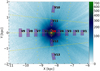 |
Fig. 1. Distribution of the sample in configuration space. We show the histogram of the 5 136 533 stars (see text) with a binning of 10×10 pc. The Sun is shown as an orange star and the GC is located at (X, Y) = (0, 0). The golden dots indicate the centres of the volumes used for the exploration in different Galactic neighbourhoods. Each radial line contains 51 volumes, and each arch at fixed radius has 21 volumes. The purple patches correspond to the sub-samples from the wider grid for which we perform a detailed study of their velocity distribution. The properties of these sub-samples are summarised in Table 1. |
Properties of the main subsamples in our study.
3. Methods
In order to detect substructures in the velocity plane (VR, Vϕ), we used the WT (Starck & Murtagh 2002). Particularly, we used the à trous algorithm, which allows the treatment of discrete data, like time series or images, without reducing the number of pixels (in our case, a 2D histogram). The WT decomposes the signal into several layers, or scales, of the same dimensions as the original, each comprising a range of frequencies (in case of time) or sizes (in the case of space). In practice, the WT returns a map of coefficients for every scale such that zero means that the signal is constant in a neighbourhood whose size is determined by the scale (as we shall see below), whereas positive coefficients correspond to overdensities and negative ones are related to underdensities. The algorithm works by successive application of smoothing filters that, when subtracting one from the previous, results in the mentioned maps of wavelet coefficients. A more detailed explanation can be found in Antoja et al. (2008, 2015) and Kushniruk et al. (2017) and references therein, where the WT is applied to similar and other cases. Here we used the multiresolution analysis (MRA) software, developed by CEA (Saclay, France) and Nice Observatory (Starck et al. 1998).
By construction, in the à trous algorithm, structures found at scale j have sizes between approximately 2j and 2j+1 pixels. The conversion from pixels to physical units (km s−1 in this case) is given simply by the bin size (Δ) of the initial 2D histogram. For our work, we chose Δ = 0.5 km s−1 pixel−1. Structures of a certain diameter D produce the highest wavelet coefficient at a scale j such that Δ2j ≤ D ≤ Δ2j+1. However, they also produce positive (negative) coefficients at other scales, especially if the overdensity (underdensity) is very significant or isolated. Other authors have focused on the upper scales (e.g. Antoja et al. 2012; Kushniruk et al. 2017), motivated not only by the typical sizes of the structures they were looking for, but also by limitations imposed by the measurement uncertainties. Now the quality of the data allows the study of smaller scales and for this work we investigated the scales j = 2, 3, 4, and 5, corresponding roughly to the velocity ranges of 2–4 km s−1, 4–8 km s−1, 8–16 km s−1, and 16–32 km s−1, respectively.
Once the WT was computed, we performed a search for local maxima at each scale. To that end, we used the method peak_local_max from the Python package Scikit-image (van der Walt et al. 2014), which returns a list of peaks separated by at least d pixels. To filter fluctuations that would correspond to a smaller scale, we used a minimum distance d = 2j pixels to retain only structures of diameters between approximately 2j and 2j+1. We note that with this approach elongated features will manifest as a trail of peaks, their precise location being along the line mostly determined by fluctuations.
Subsequently, to asses the significance of a peak, we acknowledge that the source of uncertainty in our data (the histogram) is Poisson noise. As in previous work (e.g. Antoja et al. 2008, 2012), we selected in the software the option of “Poisson with few events”, which is based on the autoconvolution histogram method (Slezak et al. 1993) and which enables the study of the low-density regions in the velocity plane without loosing precision at the centre of the distribution. In short, the method evaluates the probability (Pp) that a given coefficient is not due to Poisson noise. Since it works in the wavelet space, it takes into account the number of stars not only at the peak, but also in a vicinity whose size, again, depends on the scale. Once we specify a significance threshold, the method returns a binary value signifying whether that peak is real or not, at that level of confidence (CL). For this work, used four CLs, coded as:
0: Pp < ϵ1σ
1: ϵ1σ ≤ Pp < ϵ2σ
2: ϵ2σ ≤ Pp < ϵ3σ
3: Pp ≥ ϵ3σ,
where ϵn−σ corresponds to the area P[N(0,1) ≤ n], N(0,1) being the Normal distribution, for instance, ϵ1σ ≈ 0.841.
Additionally, we coded an alternative metric for the significance of the peaks that is the percentage of times the peak appears in a bootstrap (BS) of the data. We produced N = 1000 BS of the sample, computed the WT, and searched for all the peaks. Afterwards, and for each scale, we counted how many peaks had fallen inside a circle of radius 2j pixels around the peak detected in the data1. Subsequently, the ratio between this number and the number of BS N, gives a value between 0 (the re-sampling failed to reproduce the peak every time) and 1 (the local maximum is always reproduced). We refer to this quantity as PBS and is a measure of the probability we had of observing a particular peak in the data.
The output of the method described is a list of local maxima detected at each scale, along with the value of the WT coefficient, and the two measures of significance. We then consider a peak significant either if CL ≥ 2 or PBS ≥ 0.8. In addition, we counted the number of stars closer to the peak than the minimum distance of d = 2j pixels, since those are the source of the positive (negative) wavelet coefficient. For these stars, we also computed their median error in VR and Vϕ to quantify the data uncertainty.
4. Solar neighbourhood
In this section, we study the kinematic substructure of the SN sample described in Sect. 2. The starting point is the 2D histogram of the cylindrical velocity coordinates VR and Vϕ, which is very similar to Fig. 22 from Gaia Collaboration (2018b). After applying the methodology presented in Sect. 3 we obtain the wavelet planes (Fig. 2) and a list of significant peaks at the scales of j = 2, 3, 4, 5, corresponding to 2–4, 4–8, 8–16, and 16–32 km s−1, respectively. The colours in Fig. 2 correspond to the positive WT coefficients, while the contours are presented in two styles: solid lines delimit the positive coefficients at different levels (see caption) and dashed lines mark the negative coefficients at a single level. The negative contours help track the valleys and highlight the elongated features, but we did not plot them for the scale j = 2 to ease visualization.
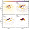 |
Fig. 2. Wavelet planes highlighting the velocity substructure in the SN at different scales. The panels correspond to scales from j = 2 (panel a) to j = 5 (panel d). The colour bar shows only the positive coefficients, just like the solid-line contours, which are shown for different percentages of the maximum coefficient at levels from 10% to 90% every 10%, plus 5% and 99%. Additionally, the negative coefficients are represented by the dashed-line contour at the −1% level. With the values used (see text), the Sun would be located at (−11,−252) km s−1 |
Panels c and d in Fig. 2 show a bi-modality and an asymmetric yet structured central distribution formed by several large-scale kinematic groups, similarly to previous studies (e.g. Dehnen 1998; Antoja et al. 2012). However, at lower scales, panels a and b, we see the recently discovered thin arches (Gaia Collaboration 2018b) crossing the velocity space in an almost horizontal direction. Immediately below, we analyse these thin arches (Sect. 4.1) and the larger-scale kinematic groups (Sect. 4.2) in more detail.
4.1. Thin arches in the velocity distribution
The precision of the Gaia data, with uncertainties in the measurements well below 1 km s−1, and the large number of stars in the SN sample (Table 1) allow us for the first time to appreciate the unprecedented detail of the velocity plane at small scales. The existence of thin arches in the Gaia DR2 data was first discovered by simple inspection of the 2D histograms of the velocity distribution. Here, the WT gives us a new representation of the data, allowing for a characterisation of the arches and, more importantly, the evaluation of their statistical significance.
Panels a and b in Fig. 2 clearly show wavelet coefficients that appear connected and organised in the above-mentioned thin arches, either composed of overdensities (positive coefficients) or underdensities (negative coefficients). The scales at which these elongated features appear indicate that they are intrinsically thin, at the level of 2–8 km s−1. Another advantage of the WT is that it highlights overdensities that are otherwise hard to discern by direct inspection of the histogram, like the arches at high |Vϕ|. Although panels a and b unveil similar kinematic substructure, some of the arches appear to be split into two at the lower scale; for example, the structure passing through (VR, Vϕ)=(0, −270) km s−1. However, for the sake of simplicity, the remainder of this subsection is devoted to the scale j = 3 alone.
Figure 3a shows the peaks detected at a scale of 4–8 km s−1. Their coordinates and characteristics are listed in Table B.1 (available at the CDS, see Appendix B). Peaks signalled with a circle are significant in terms of the Poisson noise (significance greater or equal to 2, Pp ≥ ϵ2σ); those marked with a cross are those that appeared in more than 80% of the bootstraps. As already discussed in Sect. 3, in the case of elongated structures, our peak finder procedure yields a trail of peaks. Although this method is suboptimal in detecting entire arches, we can nonetheless indirectly detect them as well as define their shape in the following manner. We selected as members of each arch the significant peaks, according either to their CL or their PBS, that show continuity in the WT coefficient. With this definition, an arch ends when the significance of the peaks we detect drops below the threshold. We note that in some cases where the connectivity of the wavelet coefficients is not clear, this grouping is slightly conjectural, yet our global conclusions do not vary. Once the peaks were selected and grouped, we fitted a second-order polynomial, Ṽϕ(VR), to each arch between its minimum and maximum VR.
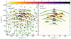 |
Fig. 3. Wavelet plane at small scale (j = 3) with the peaks and arches found. The circles correspond to those local maxima with a Poisson significance greater or equal to 2 (Pp ≥ ϵ2σ), whereas crosses correspond to those with PBS ≥ 0.8. In both cases, the diameter corresponds to Δ2j+1, indicating the highest size expected for the structures at this scale. On the right, we have associated the peaks into arches and fitted a parabola (dark green lines). The dashed grey lines then correspond to constant kinetic energy tracks. |
The arches obtained are plotted in Fig. 3b with solid dark green lines and their characteristics are given in Table 2, including the coordinates in velocity space of the first and last peaks, as well as the zero-order term of the polynomial (which corresponds to Ṽϕ(VR = 0)). In the table we also include, for reference, the name of previously known kinematic groups (discussed in Sect. 4.2) that are contained within the arches. However, it is important to note that, since past studies dealt with more circular moving groups (MGs) (due mostly to the lack of precision in the astrometry), the classical MGs and our arches are morphologically different entities.
Arches found at small scale j = 3 (4–8 km s−1).
We detected 12 arches, 6 of which cover a large range of radial velocities (A1, 4, 7, 8, 9, 12). All of them are roughly constant in azimuthal velocity. We also see that, while some parabolas are symmetrical with respect to VR = 0, others are inclined and/or present the maximum at VR ≠ 0, as already noted by Gaia Collaboration (2018b). We confirm the existence of A1 already reported by Gaia Collaboration (2018b) while A8 and A9 would correspond to the two branches of Hercules described in the same study. From all the underdensities seen in this velocity space, the most prominent known one (the gap separating Hercules from the central part) is now clearly seen running between A7 and A8–9. Another gap, just below A12, hints to a thirteenth arch, although the small number of peaks in panel (b) does not allow us to constrain it. In contrast, we see a well organised trail of peaks above A1, at Vϕ ∼ −320 km s−1, but these only have one star each and therefore we refrain from connecting them as an arch.
Several models have shown that dynamical processes like phase mixing can imprint “arc-like features” of constant radial frequency, ωR (Minchev et al. 2009; Gómez et al. 2012). Since this quantity is basically dependent on the energy for almost circular orbits, (also on angular momentum for more eccentric orbits, but not so strongly, see Dehnen 1999), these arches can be dubbed as structures of nearly constant energy. For this, we included constant energy profiles in Fig. 3b as grey dashed lines. We see how some of the arches found, such as A1 for example, are clearly compatible with having a constant kinetic energy along their trails. To quantify this similarity, we compared each parabola (evaluated with a step size of 0.1 km s−1) to the corresponding constant kinetic energy line, using the energy of the parabola at zero radial velocity, that is,  , and calculated a reduced χ2 statistic (last column in Table 2). For the short arches, based on the few peaks used for their fit, this quantity may not be representative. For the remaining arches, according to the reduced χ2, arches 1, 10 and 12 are the most compatible, while A3, 7, and 8 show the largest discrepancy with a constant energy line.
4.2. Classic and new kinematic groups
From the wavelet planes shown in panels c and d of Fig. 2, we can see the dominance of more rounded structures as the elongated features merge or fade away. Nonetheless, in panel c we can still appreciate some imprints of elongated structures. From both panels, we can clearly recognise a bi-modality formed by the centre of the distribution and the Hercules MG. Yet, in panel d the latter presents a peanut-shape, which is in fact related to two different structures, while the central over-density contains the classical MGs.
In Fig. 4 we show the significant peaks found at j = 4 where, as before, circles are related to Poisson, and crosses to bootstraps. For reference, we also plot the arches from Fig. 3b as grey lines. It becomes obvious that most of the peaks sit on top of an arch. Some of the known MGs are therefore expected to belong to the same arch, as we shall see below. All the detections in Fig. 4 are listed in Table 3, ranked according to their wavelet coefficient, that is, their relative strength at that scale. The list also contains the coordinates of the peak and the two measures of significance. The names of the objects are given according to the name in the literature that is most commonly assigned to the group (see Appendix C for details). Finally, if no match is found, we assign a new name composed of the letters “GMG” (Gaia Moving Group) and a number according to their position on the list. The table also contains the number of stars contributing to the peak, along with their median errors in the radial and azimuthal velocities.
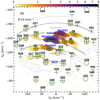 |
Fig. 4. Wavelet plane (j = 4) with the peaks found. The circles and crosses are defined as in Fig. 3. Also, solid grey lines represent the arches from the same figure. |
Groups detected at scale j = 4 (∼8–16 km s−1)
As can be seen, the known MGs (listed from selected literature in Table C.1) are among the peaks with higher coefficients, consistent with previous samples. Indeed, we confirm 22 previously known objects from Table C.1, including the most common ones. Regarding those that we do not observe, after studying each case individually we identify three reasons for this: i) we detect the MG at a smaller scale (Fig. 3a), for example HR 1614 or Hercules I; ii) the over-density is tracing an elongated feature and, as a consequence, the same structure can present the peaks at different locations depending on the sample used, for example Liang17-12 or Antoja12-15; and iii) in the case of the MG described in Dehnen (1998), their positions were later determined with higher accuracy and renamed, for example Dehnen98-9 (Hercules II) or Dehnen98-12 (ϵInd). Therefore, we can say that all peaks are confirmed in a certain way2. The most noticeable differences with previous studies are the wavelet coefficients and peaks at the less dense regions on the velocity plane, which Gaia samples now with significantly better statistics. For instance, the Bobylev16-22 (G16, or Arifyanto05) appears to be elongated and matches one of the found arches (A11), plotted in grey beneath. Its relation to groups II and III from Helmi et al. (2006), however, is still not clear. Also, Arcturus (associated to G18 and G20) is very conspicuous, while before it was only detected in specially selected samples (Williams et al. 2009). The larger wavelet coefficients for G18 compared to G20 are consistent with previous findings that Arcturus has a preferential positive VR (negative U). Besides, ϵInd (G9) appears to be more connected to Hercules than in previous studies (Liang et al. 2017), and similarly for Liang17-9 (G10). Regarding Hercules, in contrast with other studies of the SN, we detect a single peak between the two reported previously (e.g. Antoja et al. 2012; Bobylev & Bajkova 2016). A further point of interest is the connection between γ Leo (G8) and Antoja12-12 (G14), which was not observed in Antoja et al. (2012), following one of the arches (A3).
Another change with respect to past work, however, is that approximately 30 candidates MGs are found, roughly half of which have CL ≥ 2. The increase in the number of stars and the decrease in the uncertainties are the main reasons behind this findings, along with the fact that we are looking for peaks in an elongated structure (see Sect. 3). A more exhaustive cross-match with the literature is required to find previously detected groups among them and their definitive existence needs to be confirmed since the significance is not high enough. However, four of the detected groups have CL ≥ 3 (GMG1-3 and GMG6), and, remarkably, we find four (GMG-1 to -4) with strength comparable to that of the known MGs. While some of them may very well be part of the already recognised kinematic structures (e.g. G12 (GMG1) and G17 (GMG3) related to Bobylev16-22 and structure 18 from Kushniruk et al. (2017), or G13 (GMG2) related to Liang2017-9, HR 1614 and structure 19 from Kushniruk et al. (2017)), peak G19 (GMG4) is part of the newly characterised arch (A1). Finally, we observe three peaks with 1 or 2 stars (G42–44) as a result of not applying any arbitrary cut to the number of stars. These latter peaks appear significant due to their isolation from the rest of the distribution but, in any case, they do not correspond most likely to any kinematic groups, and therefore are of no interest for our study.
5. Exploring other Galactic neighbourhoods
In this section, we focus on the abundant kinematic substructure that we find in different Galactic neighbourhoods and its variation with azimuth and radius. For this exploration we used the 216 subsamples described in Sect. 2 (golden dots in Fig. 1). Most of our exploration in this section is based on the scale of 8–16 km s−1 since smaller scales appear noisier in the distant neighbourhoods for several reasons: the number of stars decreases as we move away from the Sun, the velocity uncertainties increase, and the velocity dispersion at inner Galactic radius is larger, effectively decreasing the density of stars in the velocity plane.
Figure 5 shows the wavelet plane at the scale of 8–16 km s−1 for a small sample of different Galactic neighbourhoods located at the the Solar azimuth (ϕ = 0 deg) but at different radii, going from 6.34 (V1) to 10.34 kpc (V9). It is not necessary to move very far, though, to notice changes in the substructure of the velocity plane. For example, Hercules, located at V⊙ ∼ −200 km s−1 in the SN, appears to be shifted to −220 km s−1 in V4 and to −190 km s−1 in V6. In fact, we can trace this structure from V4 to V7, but in V3 it seems to have mixed with the central part of the velocity distribution. This shift is consistent with previous findings (e.g. Antoja et al. 2012) but now we trace it farther from the Sun than ever before. The same behaviour, shifting to smaller |V⊙| when increasing R, is also observed for other structures like Sirius and Hyades. In addition, a prominent arched structure at V⊙ ∼ −260 km s−1 and positive VR is observed at V6, then more strongly at the V7 and V8 volumes. At the SN, though, it appears quite weak and only represented by the two peaks that trace A1 from Fig. 3.
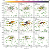 |
Fig. 5. Wavelet planes of different Galactic neighbourhoods along the zero-azimuth line. Panels a–i: correspond to the volumes V1–V9 described in Table 1. We show the coefficients in a common colour bar with the significant peaks superposed and contours in the same manner as in Fig. 2. We notice the change in colour caused by the difference in number of stars of each subsample. Also, for the SN sample, the most crowded regions of the plane saturate (cf. Fig. 4). |
The changes of the velocity substructure and especially its smooth evolution with radius can be better seen in an animation (Animation 1, see Appendix B) which considers now the 51 neighbourhoods at different radii extending in R from ∼6 kpc to ∼11 kpc at steps of 100 pc. In this animation, the downwards movement of the different kinematic structures when increasing distance from the GC can be perfectly followed as continuous passages of kinematic waves. The equivalent animations at the scales of 4–8 (Animation 2) and 16–32 km s−1 (Animation 3) show a similar evolution.
To quantify the changes in the velocity distribution with Galactocentric radius, we collected all peaks detected in the WT at scale j = 4 with CL ≥ 2 in the 51 different volumes presented in Sect. 2, and plotted their V⊙ as a function of R in Fig. 6, colour-coding the symbols according to radial velocity. With the help of the colour code, we associated all peaks that seemed to follow a common trend (both in V⊙ and VR) and linked them with a continuous solid black line, each labelled with a number. While this association of peaks may seem rather subjective, the continuity in most of the cases is beyond doubt. A simple inspection of this figure reveals a wide variety of peaks forming a general trend downwards, consistent with a decreasing |V⊙| with R as mentioned above. The expected uncertainties in the location of the peaks along the vertical axis are negligible in front of the variations observed3. We note that lines span a wide range of Galactocentric radii, meaning that the peaks at the SN have their counterparts in many other Galactic neighbourhoods, but at a different azimuthal velocity. Table 4 lists all the prominent lines in Fig. 6 where we also indicate the name of the kinematic arch or group that could be linked to each line, based on the peaks found at Solar radius (marked with squares instead of circles). Moreover, we used a linear regression to estimate the slope of the line, along with its associated uncertainty4 (penultimate column in Table 4). Overall, excluding those lines that deviate from the main trend (L1, 21, 22, 26), we observe a mean slope of 23 ± 2 km s−1 kpc−1, in good agreement with the estimation by Quillen et al. (2018b).
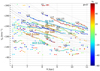 |
Fig. 6. Evolution of the rotation velocity of the kinematic substructures as a function of the radius. From all the peaks at the 51 volumes along the Sun-GC line, only significant peaks according to Poisson (CL ≥ 2) with radial velocities in the range [+60,−60] km s−1 were considered. The peaks detected at Solar radius (8.34 kpc) are shown as squares; the remaining peaks are shown as circles, linked together through solid black lines when observed to belong to the same structure (except for L13, see text). The dashed grey lines correspond to constant angular momentum tracks. |
By inspecting Table 4, we note some scatter in the measured slopes. Along with Fig. 6, we see that there seems to be two different behaviours in the slope of the most prominent lines: L5 and L9 have slopes of ∼25 km s−1 kpc−1, while L3, 10, 24, and 25 have smaller slopes between 10 and 20 km s−1 kpc−1. Developing on this, since the resonant effects of the bar and spiral arms are expected to create kinematic substructures5 that, to first order approximation and for small epicyclic amplitudes, have an almost constant vertical angular momentum LZ = RV⊙ (Sellwood 2010; Quillen et al. 2018b); we over-plot lines of constant LZ (dashed grey lines) in Fig. 6. As a result, we see how L5 and L9 follow rather well the lines of constant LZ, while other lines such as L3 and L10 do not. Moreover, the colour of the peaks reveals variations in radial velocity, which is one of the perquisites of using the WT compared to a direct plot of V⊙ against R. For most of the lines, this gradient (or oscillation in some cases) might be related to noise but, as we shall see in the discussion, for some cases like Hercules, this extra information can help us understand the origin of suchstructure.
Focusing now on individual structures that traverse the Solar radius, L3 (Sirius) is the line with the largest reach, extending from R ∼ 7.5 to R ∼ 11 kpc. Other groups with large extensions are Hyades (L6), Dehnen98-6, and Dehnen98-14 (respectively, L7 and L8) or Hercules (L9). Next to Hercules in the SN, is the MG Liang17-9 (one of the several peaks linked to A9), represented here by L10. The evolution of this group with radius differs significantly from that of Hercules, suggesting that these two substructures are different entities, with a different origin. Finally, below those two structures, we have Arcturus which, as can be seen, has been split into two lines, L13a and L13b. This is because the elongated nature of this structure, as already mentioned, makes our algorithm detect the two ends of the structure separately. We notice that, even though we detected Pleiades at SN, we do not observe any continuity with radius for this group since its relation with L25 or L7 is unclear.
We also find clear lines that do not cross the Solar radius, that is, new peaks that are detected only in extrasolar volumes. The clearest examples in outer Galactic neighbourhoods are L15–17, which correspond to the prominent arch observed in panels g and h of Fig. 5. Their connection with L2 is only truncated at two volumes, yet is traceable in Fig. 5, and the splitting can be explained using the same argument as for Arcturus. Referring to L14 and L18, there is no clear link to any of the structures detected at SN, and nonetheless they evolve similarly to the lines between them. There are also prominent new structures at inner radii such as L23 or L24, which could be associated, by visual inspection of the animation (Animation 1), to Sirius and Hyades, respectively, and L25 which presents a significantly smaller slope and does not cross the Solar radius. Finally, there are other structures with smaller extension in R, such as L1, L19 to 22, and L26, which show some continuity, meaning they are unlikely to be sporadic peaks. They are present, however, in a small range of R and depict different shapes and trends compared to the prominent lines.
Changing to the variations along azimuth, Fig. 7 shows four different wavelet planes at scale j = 4, corresponding to the volumes centred at ϕ = 10.5, 4.5, −4.5, −10.5 deg. As in previous works (Antoja et al. 2012), we do not see much variation, with only more subtle changes in the substructure compared to their evolution with R. We do observe a drift of Hercules, which moves to higher |V⊙| and becomes more prominent when increasing ϕ. There is also a structure that at V13 appears as a single, almost isolated peak around V⊙ ∼ −230, VR ∼ −40 km s−1, which corresponds to the mixture of Dehnen98-6 and Dehnen98-14, that for negative azimuth gains strength and forms an elongated structure.
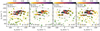 |
Fig. 7. Wavelet planes of different Galactic neighbourhoods along the arc at Solar radius. Panels a–d: correspond to the volumes V13–V10 described in Table 1. The contour levels and the symbols are defined in the same manner as in Fig. 2. |
In an analogous way to Fig. 6, in Fig. 8 we now plot V⊙ against ϕ of the peaks found in each of the 21 different Galactic neighbourhoods that cover different azimuths ϕ, for three different radii. Focusing on the middle panel, corresponding to the Solar radius, we confirm that most of the structures do not present significant variation with ϕ, except for L5 and L9 corresponding to Hyades and Hercules, respectively. The variation in azimuthal velocity in these cases is of about 13 km s−1 in 30 deg, or equivalently, ∼0.43 km s−1 deg−1, which at Solar radius means ∼3 km s−1 kpc−1, and is thus much smaller than the average 23 km s−1 kpc−1 in the radial direction. As for the variations in radial velocity revealed by the colours, we see a slight shift of the peak towards larger positive VR at ϕ = 7.5 deg for Hercules. In contrast, Sirius (L3) remains relativelyunchanged.
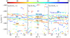 |
Fig. 8. Evolution of the rotation velocity as a function of azimuth. Here, we show the peaks of the 63 volumes (21 at each radius) that fulfil the same conditions of Fig. 6. The central panel corresponds to the exploration at the Solar radius, while in the left panel we explore an outer radius and on the right we show the results for an inner radius. |
In the left and right panels of Fig. 8, we show the azimuthal evolution in two different radii, where we see all peaks moving to larger or smaller Vϕ, in agreement with previous figures. In panel (a), corresponding to outer radius, at Vϕ ∼ −175 km s−1, the slope of Hercules with azimuth is still appreciable. In the same panel, among all the peaks at ϕ ≥ 7.5°, we distinguish a new feature at ∼−205 km s−1, worth investigating because it seems to be related to Dehnen98-14 when inspecting the animations.
6. Discussion
Although other studies have proposed links of rounded kinematic groups in the shape of a few diagonal branches (Skuljan et al. 1999; Antoja et al. 2008), ripple-like structures (Xia et al. 2015) or elongations (Kushniruk et al. 2017), the arched distribution depicted by the WT of the Gaia data is radically distinctive and clear.
Arches of almost constant energy. We have seen that some arches appearing in the SN velocity distribution have roughly the same kinetic energy at all its points in the velocity plane. This matches the models of Minchev et al. (2009) and Gómez et al. (2012) who showed how a phase-mixing process after a perturbation of the potential, possibly due to a satellite passage, naturally leads to arches in the velocity plane of nearly constant energy.
Instead, some other arches that we detect do not follow lines of constant energy and are not symmetric in their Galactocentric radial velocity. In these lines, Antoja et al. (2009) showed with simulations that a barred potential acting on a disk suffering from phase mixing will make the arches deviate from symmetry. Also, a non-axisymmetric potential (i.e. with bar and/or spiral arms) by itself can create similar arches not centred with respect to the Galactocentric radial velocity. For instance, the studies by Fux (2001), Quillen & Minchev (2005), Antoja (2010), Monari (2014) and Hattori et al. (2018) demonstrated that periodic orbits in the velocity plane have mostly an elongated locus with a peculiar arched shape. Nevertheless, while these are mostly theoretical studies analysing the regularity of the orbits, simulations of orbit integrations with realistic phase space distributions fail to distinctively populate many of these arches with particles (e.g. Antoja et al. 2011; Hattori et al. 2018), especially for spiral arms. Instead, some simulations with bars show few yet clear overdensities (and gaps) in the shape of arches (e.g. Dehnen 2000; Fux 2001). Quillen et al. 2011, 2018a) observed arches in the velocity distribution varying with position in the galaxy, which they attributed to the spiral arms.
Decrease of |V⊙| with R. We also note that most of the peaks detected by the WT decrease their azimuthal velocity with Galactocentric radius, that is, they have a negative  . Since the peaks that we detect are overdensities in phase space, their change in R is consistent with the diagonal ridges found in the R − V⊙ projection of the recent study by Antoja et al. (2018; their Fig. 3). We also confirm the large gradient measured by Quillen et al. (2018b) in the velocity of the peaks, and the extension of some of them hinted by their study. Moreover, we find that the change in R of some of the peaks, such as Hercules and Hyades for example, is consistent with them being structures of roughly constant angular momentum (LZ), i.e. following lines of constant LZ in the R − V⊙ plane, in contrast to, for instance, Sirius. This is to be expected in a resonance (Sellwood 2010; Quillen et al. 2018b) since resonant features are composed of stars following similar orbits (roughly the same eccentricity) but at different amplitudes and phases. Given that not all of the arches found in the velocity plane of the SN evolve in the same manner, this could indicate that some are due to resonances and some to a phase-mixing event. In turn, this would reduce the number of phase-mixing “waves” and, thus, increase their velocity separation. A larger separation would reduce the estimated time of perturbation of ∼2 Gyr in Minchev et al. (2009), potentially reconciling their assessment and the one by Antoja et al. (2018) from the curling of the “snail shell” in the vertical projection of phase space.
The Hercules stream. Other authors have observed a correlation between the azimuthal velocity of Hercules and R, which was used in Antoja et al. (2014) and Monari et al. (2017) to constrain the pattern speed of the bar. Our analysis returns a slope in the Vϕ–R plane for Hercules of 26.5 ± 0.2 km s−1 kpc−1, compatible with those studies. Nonetheless, we traced this trend for ∼2 kpc as opposed to the ∼0.6 kpc from previous studies. Additionally, we observe changes in the radial velocity VR of Hercules with Galactocentric distance and azimuth, which varies from ∼0 km s−1 (R ∼ 7.5 kpc) to ∼40 km s−1 (R ∼ 9 kpc). This gradient is in agreement with the behaviour predicted by Dehnen (2000), where a structure caused by the OLR of the bar evolves from zero radial velocity towards smaller |Vϕ| and positive VR with increasing radius. This model also predicts an increase of the azimuthal velocity with ϕ, which we also observe in the Gaia data. Therefore, assuming that the gap between L5 and L9 in Fig. 6 is caused by the OLR, a direct application of Eq. (6) from Quillen et al. (2018b) using the average LZ of Hercules and Hyades yields a rough estimate of the bar pattern speed of Ωb ∼ 54 km s−1 kpc−1. In contrast, Hunt & Bovy (2018) recently explained the Hercules MG with the 4:1 OLR of a slow bar. We note that the elongated feature in their Fig. 7 could also explain some of the arches that we found in the upper part of the velocity distribution. In parallel, Hattori et al. (2018) explored different models and, to our knowledge, the one that best reproduces the curvature of the gap above Hercules is their fast-bar-only. Moreover, their exploration of where in the disk the bi-modality is observed (their Fig. A.2) is more consistent with our azimuthal exploration in the case of their fast-bar-only model: both data and model show an increase of strength in Hercules with positive azimuths. Bienaymé (2018) also studied the evolution of Hercules in different Galactic neighbourhoods, but in this case our range of exploration does not allow for a comparison of the key features in his simulations. In any case, further study of the Hercules structure is necessary to settle the debate over its origin and the controversy of the bar being slow or fast, first explored by Pérez-Villegas et al. (2017).
Other kinematic substructures. Another structure with unclear origin is Arcturus, which has been linked to accreted stars from a satellite Galaxy (Navarro et al. 2004) but also to a resonance of the bar (Williams et al. 2009; Antoja et al. 2009). Here we observe that Arcturus evolves with R similarly to Hercules, pointing to a dynamical origin. We also observed other peaks that show a distinct evolution with R compared to the main groups, that is, flat, oscillating, or even increasing V⊙. Most of these have low angular momentum and therefore could have a different origin, perhaps related to accreted structures or groups in the nearby halo (Helmi et al. 1999; Koppelman et al. 2018), although their significance needs to be explored further. Finally, we recreated Figs. 6 and 8 using Bayesian distances from McMillan (2018) and observed that the differences were negligible, except for lines 21, 22, and 26 (see Table 4). With this sample we could not reconstruct any of the three, suggesting a spurious nature.
Potential biases. As can be appreciated from the strips in Fig. 1, our sample is affected by extinction. This erases the density oscillations expected in configuration space as a consequence of the conservation of number of stars and the collisionless Boltzmann equation, if we neglect minor effects from stellar birth and evolution (see this idea developed in Quillen et al. 2018b). Apart from that, as mentioned in Sect. 2, our sample is more and more dominated by giants as we move away from the Sun. Therefore, the mean age of the population can change when increasing heliocentric distances and, accordingly, our data may suffer a change in the mean velocity dispersion that can influence the detected structures in the kinematic space. In both cases, our velocity distribution could be altered, yet further work is required to fully quantify these effects.
Improvements over previous work. Previous studies with orders-of-magnitude less stars used the WT to reveal substructure in the SN that we now see by eye in the histogram (Antoja et al. 2008; Bobylev & Bajkova 2016; Kushniruk et al. 2017), making it clear that this transformation is useful in terms of detecting the substructure hidden in a poorly populated histogram. In consequence, this allows us to explore the Gaia data in depth. This exploration is inspired by, but unquestionably improves over, previous ones such as Antoja et al. (2012, 2014), who focused mostly on Hercules and for a short range of R, and Quillen et al. (2018b), who explored mostly changes in Galactic longitude but at very close distances. In comparison with other analyses (e.g. Monari et al. 2017; Antoja et al. 2018; Kawata et al. 2018), we decompose each sub-sample independently with the WT which grants us the sensitivity necessary to explore the farthest neighbourhoods and allows us to detect more and better defined ridges. Also, it introduces a third variable (VR), which in the case of Monari et al. (2017) is done through cuts in the data at the cost of reducing the number of stars.
7. Conclusions
We have studied the velocity plane in cylindrical coordinates for a Gaia sample of stars with six-dimensional phase space coordinates both in the SN, with 435 801 stars, and other Galactic neighbourhoods up to Heliocentric distances of ∼2.5 kpc. With the unprecedented number of stars and the small uncertainties in the observables, with median velocity errors of  ≤ 1 km s−1 in the vicinity of the Sun and ≤3 km s−1 for the rest of volumes, the kinematic substructures unveiled by the WT show a remarkable sharpness. We have characterised these structures, and followed their evolution with Galactocentric radius and azimuth.
The WT reveals conspicuous, thin kinematic arches with various morphologies that were not observed prior to Gaia due to resolution limitations. We find at least six long arches in the SN with a nearly constant azimuthal velocity and wide range of radial Galactocentric velocities, plus six additional shorter segments of arch. Based on the scale in the WT where they are better detected, we find that they have a width of 2–8 km s−1. Thanks to the superb isotropy of the Gaia survey and the capabilities of the WT for unveiling structures, the exploration of the substructure in the velocity distribution can now be carried out in many different Galactic neighbourhoods, that is in all directions and spanning an astonishing range of 5 kpc in Galactocentric distance. In our analysis, we see that the azimuthal velocity of the peaks detected changes strongly with Galactocentric distance at an average rate of ∼23 km s−1 kpc−1. We also see clear differences in their radial range, as some structures rapidly fade, while others can be identified in Galactic neighbourhoods 3 kpc apart. When explored as a function of Galactic azimuthal angle, most of the substructures remain constant and some present little change of the order of 3 km s−1 kpc−1, an order of magnitude smaller than the changes in Galactic radius. This is qualitatively in agreement with expectations from models of resonant structures (Antoja et al. 2011; Quillen et al. 2011) and of phase mixing (Gómez et al. 2012). Also, and although we can only explore a small portion of the MW, our results are in line with the findings of, for example, Quillen et al. (2011) and Hattori et al. (2018), who proposed, based on their simulations, the existence of streaks and gaps in the velocity distribution throughout the entire Galaxy. Overall, when looking at the evolution of the velocity plane, most of the structures shift in the vertical axis (Vϕ) at a similar rate, producing the illusion that we are indeed riding kinematic waves in the MW disk.
With the fine characterisation of the arches and ridges done in this work, we see that some of the kinematic substructures follow lines of nearly constant energy at a given volume and could be related to phase-mixing processes (Minchev et al. 2009; Gómez et al. 2012) induced, for example, by the close passage of the satellite dwarf. These coincide with the structures showing less variations in azimuthal angle, like Sirius. Others, such as Hyades or Hercules, seem to follow lines of constant angular momentum, similar to what is expected in case of resonant kinematic substructure (Sellwood 2010; Quillen et al. 2018b) induced by the bar and/or the spiral arms of our Galaxy, and also show variations with azimuthal angle. We could therefore be witnessing several mechanisms acting on the disk, as recently suggested in Antoja et al. (2018), who compared the ridges with different toy models of phase mixing and resonances, and in Trick et al. (2018) in their study of the Gaia data in action space. Here we provide additional evidence of the different dynamical characteristics of the kinematic substructures and a tentative way to differentiate between structures of different origin.
We have also shown the evolution of Vϕ for Hercules both with radius and azimuth, which is consistent with the OLR models of the Galactic bar, reaching distances of ∼1 kpc from the Sun in each direction. Moreover, we have quantified the changes in radial velocity, for the first time, at each volume along both directions. The trends seen remain consistent with the predictions for a fast bar. Our exploration has lead also to the first unambiguous extrasolar kinematic structures, that is, MGs and arches not observed (or very weak) at Solar radius. Some of these new substructures follow similar trends with Galactocentric radius and azimuth as the substructure crossing the local volume, whereas others evolve distinctively.
The Gaia mission has still some years ahead to deliver even better data, yet with the results already available it is an exciting time for both observational and theoretical research on Galactic dynamics. As an example, the structures analysed in this work and their evolution can be used to experiment with numerical and theoretical models in the context of coexisting and interacting dynamical processes.
Movies
Movie of Fig. B1 Access Supplementary Material
Movie of Fig. B2 Access Supplementary Material
Movie of Fig. B3 Access Supplementary Material
Movie of Fig. B4 Access Supplementary Material
Movie of Fig. B5 Access Supplementary Material
Here, we assume that all local maxima correspond to structures of the upper size limit.
Except for NGC1901 from Dehnen (1998) which is out of the SN sample (Kos et al. 2018).
Even though the algorithm we use does not return an error associated to the location of the peak, this can be approximated by the error on the mean velocity of the N stars composing each group: we take the maximum between their standard deviation and their uncertainty in velocity, and then divide by the square root of N. These errors are between 0.04 and 1.06 km s−1 for 80% of the peaks in the SN and between ∼0.3 and 5.0 km s−1 on average for neighbourhoods at 1 kpc from the Sun, with the low |Vϕ| region of the velocity plane being dominated by the larger errors.
In this calculation, the individual uncertainties of each peak have not been taken into account.
As Dehnen (2000) showed, gaps in the velocity distribution are easier to dynamically associate with resonances. Peaks on the other hand tend to be more unstable (Minchev et al. 2010). Nonetheless, those gaps naturally enhance the over-densities at each side of the separatrix and, as a consequence, the peaks approximately follow the gaps, which is in line with our focus on the peaks.
Acknowledgments
We would like to thank the referee for hers/his comments and knowledge on Galactic dynamics, for it has been very enriching. This work has made use of data from the European Space Agency (ESA) mission Gaia (https://www.cosmos.esa.int/gaia), processed by the Gaia Data Processing and Analysis Consortium (DPAC, https://www.cosmos.esa.int/web/gaia/dpac/consortium). Funding for the DPAC has been provided by national institutions, in particular the institutions participating in the Gaia Multilateral Agreement. This project has received funding from the University of Barcelona’s official doctoral program for the development of a R+D+i project under the APIF grant and from the European Union’s Horizon 2020 research and innovation programme under the Marie Skłodowska-Curie grant agreement No. 745617. This work was supported by the MINECO (Spanish Ministry of Economy) through grants ESP2016-80079-C2-1-R (MINECO/FEDER, UE) and ESP2014-55996-C2-1-R (MINECO/FEDER, UE) and MDM-2014-0369 of ICCUB (Unidad de Excelencia “María de Maeztu”).
References
- Antoja, T. 2010, PhD Thesis, Universitat de Barcelona [Google Scholar]
- Antoja, T., Figueras, F., Fernández, D., & Torra, J. 2008, A&A, 490, 135 [NASA ADS] [CrossRef] [EDP Sciences] [Google Scholar]
- Antoja, T., Valenzuela, O., Pichardo, B., et al. 2009, ApJ, 700, L78 [NASA ADS] [CrossRef] [Google Scholar]
- Antoja, T., Figueras, F., Romero-Gómez, M., et al. 2011, MNRAS, 418, 1423 [NASA ADS] [CrossRef] [Google Scholar]
- Antoja, T., Helmi, A., Bienayme, O., et al. 2012, MNRAS, 426, L1 [NASA ADS] [CrossRef] [Google Scholar]
- Antoja, T., Helmi, A., Dehnen, W., et al. 2014, A&A, 563, A60 [NASA ADS] [CrossRef] [EDP Sciences] [Google Scholar]
- Antoja, T., Mateu, C., Aguilar, L., et al. 2015, MNRAS, 453, 541 [NASA ADS] [CrossRef] [Google Scholar]
- Antoja, T., Helmi, A., & Romero-Gomez, M. 2018, Nature, 561, 360 [NASA ADS] [CrossRef] [Google Scholar]
- Arenou, F. 1999, in Harmonizing Cosmic Distance Scales in a Post-Hipparcos Era, eds. D. Egret, & A. Heck, ASP Conf. Ser., 167, 13 [NASA ADS] [Google Scholar]
- Astraatmadja, T. L., & Bailer-Jones, C. A. L. 2016, ApJ, 833, 119 [NASA ADS] [CrossRef] [Google Scholar]
- Bailer-Jones, C. A. L. 2015, PASP, 127, 994 [NASA ADS] [CrossRef] [Google Scholar]
- Bienaymé, O. 2018, A&A, 612, A75 [NASA ADS] [CrossRef] [EDP Sciences] [Google Scholar]
- Binney, J., Gerhard, O., & Spergel, D. 1997, MNRAS, 288, 365 [NASA ADS] [CrossRef] [Google Scholar]
- Bobylev, V. V., & Bajkova, A. T. 2016, Astron. Lett., 42, 90 [NASA ADS] [CrossRef] [Google Scholar]
- Bovy, J. 2010, ApJ, 725, 1676 [NASA ADS] [CrossRef] [Google Scholar]
- Brown, A. G. A., Arenou, F., van Leeuwen, F., Lindegren, L., & Bernacca, P. L. 1997, in Hipparcos – Venice’97, eds. R. M. Bonnet, E. Høg, P. L. Bernacca et al., ESA SP, 402, 63 [NASA ADS] [Google Scholar]
- Cui, X.-Q., Zhao, Y.-H., Chu, Y.-Q., et al. 2012, Res. Astron. Astrophys., 12, 1197 [NASA ADS] [CrossRef] [Google Scholar]
- De Silva, G. M., Freeman, K. C., Bland-Hawthorn, J., et al. 2015, MNRAS, 449, 2604 [NASA ADS] [CrossRef] [MathSciNet] [Google Scholar]
- Dehnen, W. 1998, AJ, 115, 2384 [NASA ADS] [CrossRef] [Google Scholar]
- Dehnen, W. 1999, AJ, 118, 1190 [NASA ADS] [CrossRef] [Google Scholar]
- Dehnen, W. 2000, AJ, 119, 800 [NASA ADS] [CrossRef] [Google Scholar]
- Eggen, O. J. 1996, AJ, 112, 1595 [NASA ADS] [CrossRef] [Google Scholar]
- Famaey, B., Jorissen, A., Luri, X., et al. 2005, A&A, 430, 165 [NASA ADS] [CrossRef] [EDP Sciences] [Google Scholar]
- Fux, R. 2001, A&A, 373, 511 [NASA ADS] [CrossRef] [EDP Sciences] [Google Scholar]
- Gaia Collaboration (Brown, A. G. A., et al.) 2016a, A&A, 595, A2 [NASA ADS] [CrossRef] [EDP Sciences] [Google Scholar]
- Gaia Collaboration (Prusti, T., et al.) 2016b, A&A, 595, A1 [NASA ADS] [CrossRef] [EDP Sciences] [Google Scholar]
- Gaia Collaboration (Brown, A. G. A., et al.) 2018a, A&A, 616, A1 [NASA ADS] [CrossRef] [EDP Sciences] [Google Scholar]
- Gaia Collaboration (Katz, D., et al.) 2018b, A&A, 616, A11 [NASA ADS] [CrossRef] [EDP Sciences] [Google Scholar]
- Gómez, F. A., Minchev, I., Villalobos, Á., O’Shea, B. W., & Williams, M. E. K. 2012, MNRAS, 419, 2163 [NASA ADS] [CrossRef] [Google Scholar]
- Hattori, K., Gouda, N., & Yano, T. 2018, MNRAS, submitted [arXiv:1804.01920] [Google Scholar]
- Helmi, A., White, S. D. M., de Zeeuw, P. T., & Zhao, H. 1999, Nature, 402, 53 [NASA ADS] [CrossRef] [Google Scholar]
- Helmi, A., Navarro, J. F., Nordström, B., et al. 2006, MNRAS, 365, 1309 [NASA ADS] [CrossRef] [Google Scholar]
- Hunt, J. A. S., & Bovy, J. 2018, MNRAS, 477, 3945 [NASA ADS] [CrossRef] [Google Scholar]
- Hunt, J. A. S., Bovy, J., Pérez-Villegas, A., et al. 2018, MNRAS, 474, 95 [NASA ADS] [CrossRef] [Google Scholar]
- Katz, D., Sartoretti, P., & Cropper, M. 2018, A&A, submitted [arXiv:1804.09372] [Google Scholar]
- Kawata, D., Baba, J., Ciuca, I., et al. 2018, MNRAS, 479, L108 [NASA ADS] [CrossRef] [Google Scholar]
- Koppelman, H., Helmi, A., & Veljanoski, J. 2018, ApJ, 860, L11 [NASA ADS] [CrossRef] [Google Scholar]
- Kos, J., de Silva, G., Buder, S., et al. 2018, MNRAS, 480, 5242 [NASA ADS] [CrossRef] [Google Scholar]
- Kushniruk, I., Schirmer, T., & Bensby, T. 2017, A&A, 608, A73 [NASA ADS] [CrossRef] [EDP Sciences] [Google Scholar]
- Liang, X. L., Zhao, J. K., Oswalt, T. D., et al. 2017, ApJ, 844, 152 [NASA ADS] [CrossRef] [Google Scholar]
- Luri, X., Brown, A. G. A., Sarro, L. M., et al. 2018, A&A, 616, A9 [NASA ADS] [CrossRef] [EDP Sciences] [Google Scholar]
- Majewski, S. R., Schiavon, R. P., Frinchaboy, P. M., et al. 2017, AJ, 154, 94 [NASA ADS] [CrossRef] [Google Scholar]
- McMillan, P. J. 2013, MNRAS, 430, 3276 [NASA ADS] [CrossRef] [MathSciNet] [Google Scholar]
- McMillan, P. J. 2018, Res. Notes Am. Astron. Soc., 2, 51 [NASA ADS] [CrossRef] [Google Scholar]
- Minchev, I., Quillen, A. C., Williams, M., et al. 2009, MNRAS, 396, L56 [NASA ADS] [CrossRef] [Google Scholar]
- Minchev, I., Boily, C., Siebert, A., & Bienayme, O. 2010, MNRAS, 407, 2122 [NASA ADS] [CrossRef] [MathSciNet] [Google Scholar]
- Monari, G. 2014, PhD Thesis, Rijksuniversiteit Groningen [Google Scholar]
- Monari, G., Kawata, D., Hunt, J. A. S., & Famaey, B. 2017, MNRAS, 466, L113 [NASA ADS] [CrossRef] [Google Scholar]
- Monari, G., Famaey, B., Minchev, I., et al. 2018, Res. Notes Am. Astron. Soc., 2, 32 [NASA ADS] [CrossRef] [Google Scholar]
- Navarro, J. F., Helmi, A., & Freeman, K. C. 2004, ApJ, 601, L43 [NASA ADS] [CrossRef] [Google Scholar]
- Pecaut, M. J., & Mamajek, E. E. 2013, ApJS, 208, 9 [NASA ADS] [CrossRef] [Google Scholar]
- Pérez-Villegas, A., Portail, M., Wegg, C., & Gerhard, O. 2017, ApJ, 840, L2 [NASA ADS] [CrossRef] [Google Scholar]
- Quillen, A. C., & Minchev, I. 2005, AJ, 130, 576 [NASA ADS] [CrossRef] [Google Scholar]
- Quillen, A. C., Dougherty, J., Bagley, M. B., Minchev, I., & Comparetta, J. 2011, MNRAS, 417, 762 [NASA ADS] [CrossRef] [Google Scholar]
- Quillen, A. C., Carrillo, I., Anders, F., et al. 2018a, MNRAS, 480, 3132 [NASA ADS] [CrossRef] [Google Scholar]
- Quillen, A. C., De Silva, G., Sharma, S., et al. 2018b, MNRAS, 478, 228 [NASA ADS] [CrossRef] [Google Scholar]
- Reid, M. J., Menten, K. M., Brunthaler, A., et al. 2014, ApJ, 783, 130 [Google Scholar]
- Schönrich, R., Binney, J., & Dehnen, W. 2010, MNRAS, 403, 1829 [NASA ADS] [CrossRef] [Google Scholar]
- Sellwood, J. A. 2010, MNRAS, 409, 145 [NASA ADS] [CrossRef] [Google Scholar]
- Skuljan, J., Hearnshaw, J. B., & Cottrell, P. L. 1999, MNRAS, 308, 731 [NASA ADS] [CrossRef] [Google Scholar]
- Slezak, E., de Lapparent, V., & Bijaoui, A. 1993, ApJ, 409, 517 [NASA ADS] [CrossRef] [Google Scholar]
- Starck, J.-L., Murtagh, F. D., & Bijaoui, A. 1998, Image Processing and Data Analysis, 297 [Google Scholar]
- Starck, J.-L., & Murtagh, F. 2002, Astronomical Image and Data Analysis (Berlin: Springer) [Google Scholar]
- Steinmetz, M., Zwitter, T., Siebert, A., et al. 2006, AJ, 132, 1645 [NASA ADS] [CrossRef] [Google Scholar]
- Trick, W. H., Coronado, J., & Rix, H. 2018, MNRAS, submitted [arXiv:1805.03653] [Google Scholar]
- van der Walt, S., Schönberger, J. L., The Scikit-image Contributors, et al. 2014, PeerJ, 2, e453 [CrossRef] [PubMed] [Google Scholar]
- Williams, M. E. K., Freeman, K. C., Helmi, A., & The RAVE Collaboration 2009, in IAU Symposium, eds. J. Andersen, J. Bland-Hawthorn, & B. Nordström 254, 139 [Google Scholar]
- Wilson, G. A. 1990, PhD Thesis, Kinematic and Observational Studies of Stellar Streams [Google Scholar]
- Xia, Q., Liu, C., Xu, Y., et al. 2015, MNRAS, 447, 2367 [NASA ADS] [CrossRef] [Google Scholar]
Appendix A: The proper use of parallaxes
Here we briefly discuss the recommendations given on the use of the Gaia parallaxes. For a more detailed study, we refer the reader to Luri et al. (2018). The problem of inverting the parallax is that it generates an asymmetric and biased distribution of probability for the true distance given the evidence (observations). In other words, the most probable distance is not the true distance of the star. Therefore, using summary statistics like, for instance, the mode or the mean, causes a bias in the distances derived for each star. Moreover, the simple 1/ϖ, which in a Bayesian context is equivalent to select the most likely value given a uniform prior, has been shown to be a relatively poor estimator (Brown et al. 1997; Arenou & Luri 1999; Luri et al. 2018). In addition, as shown in Luri et al. (2018), cutting in parallax relative error, σϖ/ϖ is actually far from beneficial; it can introduce an even deeper bias depending on the characteristics of the sample. In contrast, the recommendation given by the Gaia team is to work fully Bayesian, that is, not to use summary statistics and, instead, drag the Posterior probability distributions up to the quantities of interest. In this context, the results will not be a value anymore, but a whole probability density function filled with information. In general, though, it is enough to use the simple and biased estimator 1/ϖ to explore the data, always taking into account the effects it can introduce if the sample is not very close to the Sun and has large uncertainties.
Our sample, as described in Sect. 2, is for the most part made up of bright nearby stars, precisely those with the smallest mean uncertainties in the DR2 catalogue. Moreover, for nearby stars with fractional errors smaller than 0.2, the dependence on the prior is highly attenuated and the bias of using the inverse of the parallax as a distance estimator becomes negligible (e.g. Bailer-Jones 2015; Astraatmadja & Bailer-Jones 2016). Beyond that, our science case and conclusions do not rely heavily on the distance determination, and the potentially small bias does not affect the overall picture of the substructure in the kinematic plane.
As a side note, we notice that by using the Jacobian to propagate and calculate the uncertainties in the velocities, we are implicitly modelling the errors as Gaussian which is known to be false. As already mentioned, the inversion of the parallax results in an asymmetric probability distribution, also for the observed VR and V⊙. We do not impose any threshold or sigma-clipping based on this errors. In this sense, since we already selected only stars with “good” parallax, the assumption of Normality is unimportant.
Appendix B: Online material
The online data material includes a table and five animations. Table B.1 (available at the CDS) contains all the significant peaks in the SN sample at the scale 4–8 km s−1 (j = 3, see Fig. 3a), with the columns being the same as in Table 3. The animations are composed of the snapshots at different Galactocentric radius and azimuth of the WT planes, which makes it possible to visualize the evolution of the velocity distribution at a particular scale. Figures B.1–B.5 show the previews of each animations and, in the corresponding captions, the details of the scale and exploration range.
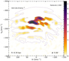 |
Fig. B.1. Preview of Animation 1. WT of the velocity plane at the scale 8–16 km s−1 at different Galactocentric distances along the GC-Sun line (ϕ = 0). |
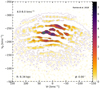 |
Fig. B.2. Preview of Animation 2. WT of the velocity plane at the scale 4–8 km s−1 at different Galactocentric distances along the GC-Sun line (ϕ = 0). |
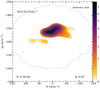 |
Fig. B.3. Preview of Animation 3. WT of the velocity plane at the scale 16–32 km s−1 at different Galactocentric distances along the GC-Sun line (ϕ = 0). |
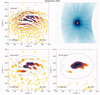 |
Fig. B.4. Preview of Animation 4. All three scales (j = 3, 4, 5) evolving simultaneously with Galactocentric distance at the GC-Sun line (ϕ = 0). |
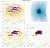 |
Fig. B.5. Preview of Animation 5. All three scales (j = 3, 4, 5) evolving simultaneously with azimuth at Solar radius (R = R⊙). |
Appendix C: List of moving groups
We compiled a list of MGs from the corresponding tables of Dehnen (1998), Antoja et al. (2012), Xia et al. (2015), Bobylev & Bajkova (2016), Liang et al. (2017) and Kushniruk et al. (2017) and list them in Table C.1. We transformed their Heliocentric velocities into Galactocentric cylindrical coordinates following the recipe given in Sect. 2. Some MGs, like Hyades or Sirius, have more than one entry since each author independently derived a different location in velocity space.
Compilation of MGs from different authors (see text).
For Kushniruk et al. (2017) we only took the new unnamed objects (with sizes between 8–16 km s−1 and 16–32 km s−1, see Kushniruk et al. 2017) in order to reduce the scatter in our table since in their study the same structure appears tabulated several times at different coordinates. Their newly found objects are label here including the scale they were found (using j as defined in Sect. 3). Regarding the elongated structures described by Xia et al. (2015), for which just the start and end points are given, we did not include them to avoid mismatches, but we considered them for the discussion. The rest of new or unnamed objects found in each author’s table are labelled as First Author + Year + Number in source table.
The names of the objects in our Table 3 are given according to the following criteria: first, we cross-matched the position of the peak detected in our data with the coordinates in the literature using a circle of radius Δ2j km s−1. Since we may have several entries for a single object, we grouped the candidates by name and counted their frequency. In cases where multiple groups were obtained, we selected the one with more counts. If we had a draw, we selected the closest one to the peak.
All Tables
All Figures
|
Fig. 1. Distribution of the sample in configuration space. We show the histogram of the 5 136 533 stars (see text) with a binning of 10×10 pc. The Sun is shown as an orange star and the GC is located at (X, Y) = (0, 0). The golden dots indicate the centres of the volumes used for the exploration in different Galactic neighbourhoods. Each radial line contains 51 volumes, and each arch at fixed radius has 21 volumes. The purple patches correspond to the sub-samples from the wider grid for which we perform a detailed study of their velocity distribution. The properties of these sub-samples are summarised in Table 1. |
| In the text | |
|
Fig. 2. Wavelet planes highlighting the velocity substructure in the SN at different scales. The panels correspond to scales from j = 2 (panel a) to j = 5 (panel d). The colour bar shows only the positive coefficients, just like the solid-line contours, which are shown for different percentages of the maximum coefficient at levels from 10% to 90% every 10%, plus 5% and 99%. Additionally, the negative coefficients are represented by the dashed-line contour at the −1% level. With the values used (see text), the Sun would be located at (−11,−252) km s−1 |
| In the text | |
|
Fig. 3. Wavelet plane at small scale (j = 3) with the peaks and arches found. The circles correspond to those local maxima with a Poisson significance greater or equal to 2 (Pp ≥ ϵ2σ), whereas crosses correspond to those with PBS ≥ 0.8. In both cases, the diameter corresponds to Δ2j+1, indicating the highest size expected for the structures at this scale. On the right, we have associated the peaks into arches and fitted a parabola (dark green lines). The dashed grey lines then correspond to constant kinetic energy tracks. |
| In the text | |
|
Fig. 4. Wavelet plane (j = 4) with the peaks found. The circles and crosses are defined as in Fig. 3. Also, solid grey lines represent the arches from the same figure. |
| In the text | |
|
Fig. 5. Wavelet planes of different Galactic neighbourhoods along the zero-azimuth line. Panels a–i: correspond to the volumes V1–V9 described in Table 1. We show the coefficients in a common colour bar with the significant peaks superposed and contours in the same manner as in Fig. 2. We notice the change in colour caused by the difference in number of stars of each subsample. Also, for the SN sample, the most crowded regions of the plane saturate (cf. Fig. 4). |
| In the text | |
|
Fig. 6. Evolution of the rotation velocity of the kinematic substructures as a function of the radius. From all the peaks at the 51 volumes along the Sun-GC line, only significant peaks according to Poisson (CL ≥ 2) with radial velocities in the range [+60,−60] km s−1 were considered. The peaks detected at Solar radius (8.34 kpc) are shown as squares; the remaining peaks are shown as circles, linked together through solid black lines when observed to belong to the same structure (except for L13, see text). The dashed grey lines correspond to constant angular momentum tracks. |
| In the text | |
|
Fig. 7. Wavelet planes of different Galactic neighbourhoods along the arc at Solar radius. Panels a–d: correspond to the volumes V13–V10 described in Table 1. The contour levels and the symbols are defined in the same manner as in Fig. 2. |
| In the text | |
|
Fig. 8. Evolution of the rotation velocity as a function of azimuth. Here, we show the peaks of the 63 volumes (21 at each radius) that fulfil the same conditions of Fig. 6. The central panel corresponds to the exploration at the Solar radius, while in the left panel we explore an outer radius and on the right we show the results for an inner radius. |
| In the text | |
|
Fig. B.1. Preview of Animation 1. WT of the velocity plane at the scale 8–16 km s−1 at different Galactocentric distances along the GC-Sun line (ϕ = 0). |
| In the text | |
|
Fig. B.2. Preview of Animation 2. WT of the velocity plane at the scale 4–8 km s−1 at different Galactocentric distances along the GC-Sun line (ϕ = 0). |
| In the text | |
|
Fig. B.3. Preview of Animation 3. WT of the velocity plane at the scale 16–32 km s−1 at different Galactocentric distances along the GC-Sun line (ϕ = 0). |
| In the text | |
|
Fig. B.4. Preview of Animation 4. All three scales (j = 3, 4, 5) evolving simultaneously with Galactocentric distance at the GC-Sun line (ϕ = 0). |
| In the text | |
|
Fig. B.5. Preview of Animation 5. All three scales (j = 3, 4, 5) evolving simultaneously with azimuth at Solar radius (R = R⊙). |
| In the text | |
Current usage metrics show cumulative count of Article Views (full-text article views including HTML views, PDF and ePub downloads, according to the available data) and Abstracts Views on Vision4Press platform.
Data correspond to usage on the plateform after 2015. The current usage metrics is available 48-96 hours after online publication and is updated daily on week days.
Initial download of the metrics may take a while.