| Issue |
A&A
Volume 618, October 2018
|
|
|---|---|---|
| Article Number | A39 | |
| Number of page(s) | 13 | |
| Section | Cosmology (including clusters of galaxies) | |
| DOI | https://doi.org/10.1051/0004-6361/201833371 | |
| Published online | 15 October 2018 | |
Measuring turbulence and gas motions in galaxy clusters via synthetic Athena X-IFU observations
1
Dipartimento di Fisica e Astronomia, Università di Bologna, via Gobetti 93, 40127 Bologna, Italy
e-mail: mauro.roncarelli@unibo.it
2
Istituto Nazionale di Astrofisica (INAF) – Osservatorio di Astrofisica e Scienza dello Spazio (OAS), via Gobetti 93/3, 40127
Bologna, Italy
3
Department of Astrophysical Sciences, Princeton University, 4 Ivy Lane, Princeton, NJ, 08544-1001 USA
4
Istituto Nazionale di Fisica Nucleare (INFN) – Sezione di Bologna, viale Berti Pichat 6/2, 40127 Bologna, Italy
5
Dipartimento di Fisica dell’Università di Trieste, Sezione di Astronomia, via Tiepolo 11, 34131 Trieste, Italy
6
Istituto Nazionale di Astrofisica (INAF) – Osservatorio Astronomico di Trieste, via Tiepolo 11, 34131 Trieste, Italy
7
Harvard-Smithsonian Center for Astrophysics, 60 Garden Street, Cambridge, MA, 02138 USA
8
IRAP, Université de Toulouse, CNRS, UPS, CNES, 31042 Toulouse, France
Received:
5
May
2018
Accepted:
2
July
2018
Context. The X-ray Integral Field Unit (X-IFU) that will be on board the Athena telescope will provide an unprecedented view of the intracluster medium (ICM) kinematics through the observation of gas velocity, ν, and velocity dispersion, w, via centroid-shift and broadening of emission lines, respectively.
Aims. The improvement of data quality and quantity requires an assessment of the systematics associated with this new data analysis, namely biases, statistical and systematic errors, and possible correlations between the different measured quantities.
Methods. We have developed an end-to-end X-IFU simulator that mimics a full X-ray spectral fitting analysis on a set of mock event lists, obtained using SIXTE. We have applied it to three hydrodynamical simulations of a Coma-like cluster that include the injection of turbulence. This allowed us to assess the ability of X-IFU to map five physical quantities in the cluster core: emission measure, temperature, metal abundance, velocity, and velocity dispersion. Finally, starting from our measurements maps, we computed the 2D structure function (SF) of emission measure fluctuations, ν and w, and compared them with those derived directly from the simulations.
Results. All quantities match with the input projected values without bias; the systematic errors were below 5%, except for velocity dispersion whose error reaches about 15%. Moreover, all measurements prove to be statistically independent, indicating the robustness of the fitting method. Most importantly, we recover the slope of the SFs in the inertial regime with excellent accuracy, but we observe a systematic excess in the normalization of both SFν and SFw ascribed to the simplistic assumption of uniform and (bi-)Gaussian measurement errors.
Conclusions. Our work highlights the excellent capabilities of Athena X-IFU in probing the thermodynamic and kinematic properties of the ICM. This will allow us to access the physics of its turbulent motions with unprecedented precision.
Key words: galaxies: clusters: intracluster medium / galaxies: clusters: general / X-rays: galaxies: clusters / intergalactic medium / methods: numerical / techniques: imaging spectroscopy
© ESO 2018
1. Introduction
The Advanced Telescope for High ENergy Astrophysics1 (Athena) is the next-generation, groundbreaking X-ray observatory mission selected by ESA to study the Hot and Energetic Universe; its launch is expected in 2028 (Nandra et al. 2013). With its two instruments, the Wide Field Imager and the X-ray Integral Field Unit (X-IFU; Barret et al. 2016), Athena will provide a crucial window on the X-ray sky, strongly complementing the other next-generation telescopes covering the lower energy bands (e.g., ALMA, ELT, Euclid, JWST, SKA). In particular, the X-IFU will consist of a cryogenic X-ray spectrometer with a large array of transition-edge sensors, with the goal of achieving 2.5 eV spectral resolution, with 5″ pixels, over a field of view (FOV) of about 5 arcmin. The X-IFU is expected to deliver superb spatially resolved high-resolution spectra, opening the era of imaging spectroscopy in the X-ray band.
One of the primary goals of Athena X-IFU is probing the (astro)physics of the diffuse plasma which fills the potential wells of galaxy clusters (Ettori et al. 2013; Croston et al. 2013; Pointecouteau et al. 2013), also known as the intracluster medium (ICM). The ICM, which formed during the cosmological gravitational collapse in the growing dark matter halo (e.g., Planelles et al. 2017), accounts for most of the baryonic mass of a massive galaxy cluster (∼12 − 15% of the total mass of ∼1015 M ⊙), with typical electron temperatures and densities in the core of Te ∼ 5 − 10 keV and ne ∼ 10−2 − 10−3 cm−3, respectively. While the thermodynamics of the ICM, particularly in the core region (< 0.1 R vir), has been fairly well constrained by XMM-Newton and Chandra, its kinematics remains very poorly understood.
On the theoretical side, cosmological simulations show that the ICM is continuously stirred by the accretion of substructures or merger events at 100 s kpc scale (e.g., Dolag et al. 2005; Vazza et al. 2011a; Lau et al. 2009, 2017) and by the self-regulated active galactic nucleus (AGN) feedback in the inner core (e.g., Gaspari & Sądowski 2017 for a brief review of the self-regulated cycle). In both cases, the injected turbulence is subsonic in the ICM with a few 100 km s−1 magnitude. Until recently the observational constraints on ICM gas motions have been indirectly derived from measurements of X-ray surface brightness fluctuations (e.g., Schuecker et al. 2004; Churazov et al. 2012; Gaspari & Churazov 2013; Zhuravleva et al. 2015; Walker et al. 2015; Hofmann et al. 2016), resonant scattering (e.g., Churazov et al. 2004; Ogorzalek et al. 2017; Hitomi Collaboration et al. 2018), and Sunyaev–Zeldovich fluctuations (Khatri & Gaspari 2016). At the same time, XMM-Newton RGS grating observations have shown the potential for high-resolution spectroscopy to directly infer gas motions from the spectral line broadening, setting significant upper limits on the ICM turbulence in several cool-core clusters (e.g., Sanders et al. 2010; Bulbul et al. 2012; Sanders & Fabian 2013; Pinto et al. 2015). In its brief life, only the Soft X-ray Spectrometer Calorimeter on board the Hitomi satellite has given us the first direct detection of the line-of-sight ICM velocity dispersion in the inner 100 kpc of the Perseus cluster, showing turbulent velocities on the order of 150 km s−1 (Hitomi Collaboration et al. 2016, 2018). A similar level of chaotic motions has been confirmed via the well-resolved velocity dispersion of the ensemble Hα + [NII] warm gas condensing out of the turbulent ICM (Gaspari et al. 2018).
Given the vastly improved capabilities compared with its predecessor XMM-Newton RGS (see, e.g., Sanders & Fabian 2013), X-IFU will be able to directly test turbulent and bulk motions via two observables: the broadening and the shift of the centroids of the emission lines in the X-ray band (such as the Fe, L, and K complexes; e.g., Inogamov & Sunyaev 2003). This will allow a direct measurement of motions that are known to drastically affect the physics of the ICM inducing cosmic ray re-acceleration (e.g., Brunetti et al. 2001; Petrosian 2001; Eckert et al. 2017b; Bonafede et al. 2018), thermal instability (e.g., Gaspari 2015; Voit 2018), and magnetic field amplification (e.g., Cho et al. 2009; Santos-Lima et al. 2014; Beresnyak & Miniati 2016). Moreover, the understanding of ICM kinematics, combined with the more traditional techniques of density and temperature mapping, has the potential to improve the robustness of cluster mass measurements. While current X-ray analyses have to rely on the hydrostatic equilibrium hypothesis, it may lead to underestimates on the order of 10–20% (see, e.g., Piffaretti & Valdarnini 2008; Lau et al. 2009; Rasia et al. 2012; Shi et al. 2016; Biffi et al. 2016), new constraints on the kinematics of cluster plasma will allow us to test them directly. Finally, these new observables will improve our knowledge of cluster formation and structure assembly up to the virial regions where the ICM becomes more inhomogeneous and connects with the large-scale structure of the Universe (see, e.g., Roncarelli et al. 2006, 2013; Vazza et al. 2011b; Eckert et al. 2015, 2018).
The introduction of imaging spectroscopy, with its increased amount of information, will require the definition of new methods of X-ray data analysis. A crucial point in order to fully exploit this large set of high-resolution spectra is the assessment of biases and systematics that may arise from instrumental effects and limits of the X-ray fitting methods. In this work, we anticipate the key impact of Athena X-IFU by running for the first time a series of end-to-end advanced synthetic observations, starting from hydrodynamical simulations, carefully including all observational effects (i.e., projection, noise, instrumental background) down to the measurement of all physical quantities via spectral fitting. In this exploratory investigation we emphasize the intrinsic physical quantity definitions, and we investigate possible systematic biases and uncertainties on their retrieval as well as statistical correlations of their measurements. All these properties must be first precisely assessed in order to provide robust physics estimates on the nature of turbulence and bulk motions that remain the ultimate goals of X-IFU observations. Overall, this study will be invaluable to fully leverage the X-ray capabilities of the next-generation Athena observatory, at the same time helping the community to find the more effective path to advance the X-ray ICM field in the next decade.
The paper is structured as follows. Section 2 reviews the high-resolution hydrodynamical 3D simulations used in this study and how we model the Athena X-IFU synthetic observations. Section 3 presents the results of the synthetic data analysis, while carefully dissecting all the biases and uncertainties. In Sect. 4, we make extensive use of structure functions (mathematically tied to power spectra) to assess the main ICM kinematics and thermodynamics at varying scales. Finally, we summarize and present concluding remarks in Sect. 5. Throughout the paper we assume a flat ΛCDM cosmological model, with Ωm = 0.3, ΩΛ = 0.7, and H0 = 70 km s−1 Mpc−1. When quoting metal abundances, we refer to the solar value (Z⊙) as measured by Anders & Grevesse (1989). To avoid confusion with the error quotations, we use ν to indicate velocities and w (instead of σν, for example) for velocity dispersions, and refer to their errors as σν and σw, respectively. Quoted errors indicate ±1σ uncertainties.
2. Models and method
2.1. High-resolution hydrodynamical simulations
The starting point of our work is the output of the high-resolution hydrodynamical simulations of galaxy clusters presented in Gaspari & Churazov (2013) and Gaspari et al. (2014), hereafter G13 and G14. Here we briefly summarize their main features and ingredients. We refer the interested reader to G13 for the details and in-depth discussions of the related numerics and physics.
The G13 and G14 simulations have been structured to be controlled experiments of key plasma physics in an archetypal massive and hot galaxy cluster similar to the Coma cluster, with virial mass M vir ≈ 1015 M ⊙ and R vir ≈ 2.9 Mpc (R 500 ≈ 1.4 Mpc). The initial density and temperature profiles of the hot plasma are set to match deep XMM-Newton observations of Coma, which shows characteristic central density n e, 0 ≃ 4 × 10⁻³ (with beta profile index β = 0.75) and flat core temperature T 0 = 8.5 keV (with declining large-scale profile ∝r −1). Given the large core temperature, Coma is the ideal laboratory for testing the effect of plasma transport mechanisms as thermal conduction. The 3D box has a side length ≃1.4 Mpc. We adopted a uniform, fixed grid of 5123 to accurately study perturbations and turbulence throughout the entire volume, reaching a spatial resolution l pix ≃ 2.7 kpc.
By using a modified version of the Eulerian grid code FLASH4 (with third-order unsplit piecewise parabolic method), we solve the 3D equations of hydrodynamics for a realistic two-temperature electron-ion plasma, testing different levels of turbulence injection and electron thermal conduction G13 Eqs. (3)–(7). The plasma is fully ionized with atomic weight for electrons and ions of μ i ≃ 1.32 and μ e ≃ 1.16, respectively, providing a total gas molecular weight μ ≃ 0.62. The ions and electrons equilibrate via Coulomb collisions on a timescale ≳50 Myr in the diffuse and hot ICM (G13 Sect. 2.5).
Turbulence is injected in the cluster via a spectral forcing scheme based on an Ornstein–Uhlenbeck random process (G13 Sect. 2.3), which reproduces experimental turbulence structure functions (Fisher et al. 2008). The stirring acceleration is first computed in Fourier space and then directly converted to physical space. Modeling the action of mergers and cosmic inflows (e.g., Lau et al. 2009; Miniati 2014), the injection scale is set to have a peak at L ≈ 600 kpc, thus exploiting the full dynamical range of the box. By setting the energy per mode, we can control the injected turbulence velocity dispersion or 3D Mach number, ℳ = w/cs, which is observed to be subsonic in the ICM (e.g., Pinto et al. 2015; Khatri & Gaspari 2016). We considered three different values of the Mach number: ℳ = 0.25, 0.50, 0.75 (the Coma sound speed is cs ≈ 1500 km s−1). We evolve the system for at least two eddy turnover times (∼2 Gyr for the slowest models), tturb ∼ L/w, to achieve a statistical steady state of the turbulent cascade. The turbulent diffusivity at injection can be defined as Dturb ≈ w L.
In this paper, we only analyze the hydro runs with highly suppressed conduction (f = 0). Recent constraints, for example the survival of ram-pressure stripped group tails (De Grandi et al. 2016; Eckert et al. 2017a) and the presence of significant relative density and surface brightness fluctuations in the bulk of the ICM (e.g., G13; Hofmann et al. 2016; Eckert et al. 2017), indicate a high level of suppression (f ≲ 10−3) compared with the classic Spitzer (1962) value. Highly tangled magnetic fields and plasma micro-instabilities (e.g., firehose and mirror) conspire to reduce the electron (and ion) mean free path well below the collisional Coulomb scale.
2.2. Modeling X-IFU observations
In this section we describe our synthetic observation method, which ultimately generates a set of realistic mock X-IFU event lists. The first step consists in creating for every hydrodynamical simulation an (x, y, E) spectroscopic data cube that contains the ideal imaging and spectra of photons that impact the telescope (i.e., without instrumental effects) as a function of sky position (x, y) and energy, E (see a similar procedure described in Roncarelli et al. 2012). In a second phase we use this information as an input for the SImulation of X-ray TElescopes (SIXTE, Wilms et al. 2014) code, the official simulator of the Athena instruments. From that we finally obtain a set of mock X-IFU event lists.
Starting from the outputs of the hydrodynamical code, we model the expected X-ray emission of each simulated  cell. We place our simulated clusters at a comoving distance corresponding to z
0 = 0.1 and consider the telescope to be oriented along one of the simulation axes to facilitate the line-of-sight integration. With this configuration the 1.4 Mpc cube width corresponds to 12.6 arcmin, so that the width of the X-IFU FOV (∼5 arcmin) corresponds to ∼40% of the cube side. On the other hand, each volume element is 1.5 arcsec wide: this means that considering the SIXTE detector configuration, an X-IFU pixel (4.38 arcsec wide) encloses on average ∼8.5 different simulation cells, i.e., more than 4000 volume elements when considering the integration along the line of sight.
cell. We place our simulated clusters at a comoving distance corresponding to z
0 = 0.1 and consider the telescope to be oriented along one of the simulation axes to facilitate the line-of-sight integration. With this configuration the 1.4 Mpc cube width corresponds to 12.6 arcmin, so that the width of the X-IFU FOV (∼5 arcmin) corresponds to ∼40% of the cube side. On the other hand, each volume element is 1.5 arcsec wide: this means that considering the SIXTE detector configuration, an X-IFU pixel (4.38 arcsec wide) encloses on average ∼8.5 different simulation cells, i.e., more than 4000 volume elements when considering the integration along the line of sight.
For each of the 5123 cubic cells we consider its density ρ
i
, its (electron) temperature T
i
, and its velocity ν
i
along the line of sight provided by the simulation, and use them to compute the expected emission spectra assuming an APEC model (version 2.0.2, Smith et al. 2001). In detail, we use the XSPEC software (version 12.9.0i) and fix the effective redshift to (1)
(1)
being c the speed of light in vacuum. The normalization2 is then fixed to (2)
(2)
being d c (z i ) the comoving distance, and where n e, i and n H, i are the electron and hydrogen number density derived from ρ i assuming a primordial He mass abundance of Y = 0.24. Since our hydrodynamical simulations do not provide a self-consistent metal enrichment scheme, our spectra are computed assuming a uniform metal abundance of Z = 0.3 Z ⊙. We also fix the Galactic hydrogen column density to N H = 5 × 1020 cm−2, which corresponds to an average absorption value. After computing the spectra for every cell, we obtain the (x, y, E) data cube by integrating the spectra along the line of sight. This is done for each of the three simulation runs. Regarding the properties of emission-lines, which is the most important aspect of our work, we note that while thermal broadening is modeled by the APEC model itself and is derived from the cell temperature T i , velocity or turbulence broadening is not a direct input of our simulations; instead, it emerges in the projection phase as a result of the superimposition of spectra with different peculiar velocities ν i provided by the hydrodynamical simulations. Our approach, therefore, mimics the real physical process without introducing any further assumptions. We fix the energy binning of our (x, y, E) data cubes to 1 eV uniformly from 2 to 8 keV, enough to sample the expected 2.5 eV X-IFU energy resolution.
This set of data is then used as input for the SIXTE software. Following the specifications of the SIXTE manual3 (see also Schmid et al. 2013), each data cube is assumed to be placed in a given position in the sky, defined by the coordinate of its center. This allows us to define a set of sources that cover the full FOV of X-IFU, each of which has a proper spectrum. These sources are then processed by the SIXTE software, assuming the most recent X-IFU characteristics, to provide a mock observed event list. Specifically, starting from the input spectra SIXTE performs a Monte Carlo generation of photons, assumed to impact the telescope with given position, energy, and time. Each mock photon is then processed to derive whether it is detected, and if so the position and energy measured by the detector are saved. This process considers the PSF of the instrument, its response function, the vignetting due to the telescope optics, and other detector effects such as its geometry, filling-factor, cross-talk, and pile-up. A more detailed explanation of the implementation of these effects can be found in the SIXTE manual and paper (Wilms et al. 2014).
In order to reach the same statistical significance, we vary the exposure time t exp for each of the three simulated observations to obtain a total number of N ph = 18 × 106 photons in the 2–8 keV energy range. Given the different thermodynamical properties of the simulations (see G13), this translates into a factor of ∼2.5 difference in t exp between the ℳ = 0.75 and the ℳ = 0.25 simulations. We verified that in order to reach this number of photon counts with a T ∼ 8 keV cluster at z = 0.1 we would need t exp ≃ 2 Ms, thus significantly higher with respect to the predictions of realistic X-IFU observations. On the other hand, this allows us to substantially reduce the resulting statistical errors and to provide a better characterization of the systematics, which is the scope of the present work.
2.3. Measuring the ICM physical parameters
Our three mock event lists undergo a full X-ray analysis. For each simulation we divide the X-IFU FOV using the Voronoi tessellation method (Cappellari & Copin 2003) in regions containing about 30 000 photons each: this translates into about 600 pixels. Then we extract the spectra corresponding to each Voronoi region and, after binning them according to the X-IFU response function, we fit them using XSPEC (Cash statistics). To account for the effect of vignetting, we consider a different response function for each spectra: this is done by modifying the on-axis X-IFU response function according to the position of the center of the Voronoi region, following the same vignetting function as was implemented in SIXTE. This step leads to a reduction in the effective area of 4%–8%, depending on the energy, in the external regions of the FOV, enough to induce a significant systematic effect if not correctly accounted for. Instead, we neglect the effect of photon pile-up after verifying that it has a small impact in our final mock event lists. Once the response function is computed, we fit each spectra through the full 2–8 keV range using XSPEC assuming a BAPEC model with five free-parameters: normalization, temperature, metal abundance, redshift, and velocity broadening: this procedure is done “blind”, i.e., without any a priori knowledge about the input physical conditions; the only exceptions are the H column density, which we fix to the input value of N H = 5 × 1020 cm−2, and the value of z 0. We also point out that by adopting a single metallicity value, we are implicitly assuming that the abundance ratios of the different ions (O/Fe, Si/Fe, and so on) have solar values. We show in Fig. 1 a sketch of the fitting procedure and of its results applied to one of the ℳ = 0.75 mock spectra.
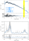 |
Fig. 1. Example of a mock X-IFU spectrum extracted from the ℳ = 0.75 run and of its fitting procedure. Top panel: spectral data points with error bars (black crosses) in the whole fitting interval and best-fit model (blue line). Fit results, with errors, for the five free parameters are indicated in the box in the bottom left. The value of ν is obtained assuming the true redshift, z 0 = 0.1, is known. The bottom subpanel shows the residuals with respect to the model. Bottom panel: same as top panel, but zooming on the 6–6.4 keV energy range (highlighted in yellow in the top panel) where the most prominent emission lines are present. In this case the features correspond to the blending of the Fe XXV and Fe XXVI K complexes. In both panels data points have been rebinned for display purposes. The plot scaling for the spectra is logarithmic in the top panel and linear in the bottom panel. |
The fitting procedure proves to be robust and converges to a result without issues for the majority of the fitted spectra. In about 3% of the cases an error occurs in the computation of the confidence regions4; this is due both to the complexity of the fitting procedure (i.e., C-stat minimization on a five-parameters space) and to the intrinsic thermodynamical inhomogeneity of the emitting gas. To avoid possible issues we removed these cases from our analysis.
3. Results
3.1. Intrinsic quantities definitions
We show in Fig. 2 (bottom panels) the X-IFU maps with the results of our fitting procedure for the ℳ = 0.75 run. Measured velocity maps were obtained from the redshift nominal value by reverting Eq. (1). We compared these maps with those of the corresponding projected quantities computed directly from the simulations (top panels), averaging in the volume enclosed in the same line of sight. From the various possible definitions of average (i.e., mass-weighted, emission weighted), we chose the ones that show a better correlation with the measured values. In detail for each X-IFU pixel we compute the following quantities:
-
spectroscopic-like temperature (Mazzotta et al. 2004),
 (4)
(4)
In the above formulas on the left-hand side we show the analytical definitions with line-of-sight integrals, and on the right-hand side the equivalent numerical definitions with the index i running through all the cells along the full length of the simulation box (≃1.4 Mpc). While the definition of EM (directly connected to the spectrum normalization, as in Eq. (2)) and Tsl are already widely adopted in X-ray astrophysics, only recently some works (see, e.g., Biffi et al. 2013) have proved how the last two quantities correlate with the centroid-shift and line broadening measurements better than the equivalent mass-weighted values. A visual inspection shows an excellent agreement of both emission measure and velocity. In particular, it is important to note that with our mock measurements we are able to recover the details of the line-of-sight velocity field with great accuracy. In addition, measured temperature maps show a good agreement with spectroscopic-like temperature maps. Broadening measurements, on the other hand, prove to be the most challenging even though both the average broadening value and the main features of the wew maps are appropriately recovered.
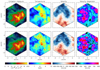 |
Fig. 2. X-IFU maps showing input quantities (top panels) vs. measured ones (bottom) for the ℳ = 0.75 model. Input quantities are derived directly from the simulation output, considering the average along the line of sight enclosed by the X-IFU pixel (4.38 arcsec wide) and computed with the definitions in Eqs. (3)–(6). For measured quantities we show the nominal value derived from the fitting of our synthetic spectra (see text for details) in the corresponding 588 Voronoi regions (≈125 arcsec2 each). From left to right: emission measure, gas temperature (spectroscopic-like, in the top panel), velocity, and velocity dispersion (both emission-weighted, in the top panels). |
3.2. Biases and uncertainties
In this section we analyze the accuracy of the X-ray measurements by comparing them with the input quantities computed from the simulations with the definitions of Eqs. (3)–(6). In the following, we will distinguish between biases, i.e., possible systematic offsets in the measurements, and systematic errors/uncertainties, i.e., the irreducible scatter between measurements and the corresponding theoretical values. For the analysis presented here, the latter values are associated with the limits of the assumption of a five-parameter model adopted in our fitting procedure in the case of ICM mixing. These errors may eventually be reduced by adopting more complicated models (such as allowing multiple ICM components).
We show in Fig. 3 the relation among the results obtained from the fitting procedure, with errors, and those extracted from the simulations for the ℳ = 0.75 model (the red solid lines indicate the identity). In Appendix A we show the same plots for the other two simulations. The values on the x-axes were computed by applying the formulas of Eqs. (3)–(6) directly to the input hydrodynamical simulation in the volume corresponding to the Voronoi region of the measurements projected along the line of sight. As expected from Fig. 2, emission measure and velocity show the most precise measurements. In particular, we point out that the comparison between the fit result and vew shows no significant bias even for high values of velocity. Temperature measurements show also a good agreement with Tsl, with a small hint of temperature overestimation for the few regions with Tsl < 6.5 keV; this may indicate that in the lower temperature regimes the definition of Tsl provided in Eq. (4), which was optimized for CCDs, might need to be revisited. As expected, the velocity dispersion measurements also show good agreement with the corresponding wew, with possibly a hint of overestimation for high wew values. We note that in this case errors in the measurements may vary considerably from σw ≈ 40 km s−1 to σw ≈ 100 km s−1. In the top left corner of each plot we show the Spearman correlation rank between measured and real quantities. In all cases the correlation is extremely high. Indeed, we obtain an almost perfect correlation (rS ≈ 1) for emission measure and velocity, to rS ∼ 0.9 for temperature, and rS ∼ 0.75 for velocity dispersion. This confirms the accuracy of the measurements of the different physical quantities.
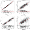 |
Fig. 3. Scatter plots of observed quantities with errors (y-axis) vs. input projected values (x-axis) for the ℳ = 0.75 simulation. Top left: emission measure. Top right: temperature vs. spectroscopic-like temperature. Bottom left: velocity vs. emission-weighted velocity. Bottom right: velocity dispersion vs. emission-weighted velocity dispersion. In each plot the red solid lines shows the identity and the bottom panel shows the residuals in units of σ. In the top left corner of each panel we show the Spearman correlation rank between observed and input values. |
The quantification of these results is shown in Table 1 together with other statistical estimates described and discussed in the following. All results are reported for the three different simulation setups, and are also related to the metallicity. We define the average bias (third column) as (7)
(7)
where m i and t i are the sets of measured and true projected quantities extracted from the simulations Eqs. (3)–(6). Remarkably, biases in the measurements are almost negligible for all quantities: this is both an indication of the robustness of the fitting procedure and of the suitability of the definitions of Eqs. (3)–(6) in representing the observationally derived values. On the other hand, we verified that mass-weighted quantities are, instead, significantly different with respect to measured ones, with mass-weighted temperature and velocity dispersion biased high by ∼0.2 keV and ∼40 km s−1, respectively. Mass weighted velocities are instead about 30% smaller than observed ones (see also Biffi et al. 2013).
In the central columns of the table, we quote the total, statistical, and systematic errors of the measured quantities computed in the following way. Total errors are computed as (8)
(8)
Statistical errors are instead derived from the fit errors with the following formula (see details in Appendix B): (9)
(9)
This expression is also appropriate for asymmetric errors, with σ
1 and σ
2 being the left and right errors, respectively. Thus, in our case it provides a better description with respect to the simple Gaussian error estimates. Systematic errors are then simply derived as (10)
(10)
and provide an indication of the expected scatter associated with the model uncertainty.
For emission measure, the number counts adopted in our simulations are enough to reduce statistical errors below systematic ones (∼3%). The latter are associated with the X-IFU point spread function that scatters photons in the areas close to the borders of the Voronoi regions, and would be negligible with a more realistic exposure time. This also causes the highest EM measurements to be slightly underestimated, as it appears in Fig. 3. Most interestingly, we observe that the values of σ ν, sys increase for larger Mach numbers, going from 25 km s−1 for ℳ = 0.25 to about 80 km s−1 for ℳ = 0.75, due to the larger gas mixing. The same applies for σ w, sys, which grows proportionally with ⟨w ew⟩ and with the Mach number, and remains approximately 15% of the average value.
In order to evaluate the accuracy of the errors provided by our fitting procedure, for each measurement we compute its normalized residual (11)
(11)
being σ 1, 2 the left and right measurement errors provided by the fit. We then use the distributions of the χ values to determine two statistical estimators. First, we identify the outliers by applying a 2.5σ clipping to the different distributions and compute its fraction. Then we compute the fraction of values in the range [ − 1, 1]: this represents the fraction of points within 1σ of the true value. The results are listed in the last two columns of Table 1. The outliers fraction for the measurements of EM, T, and Z are comparable to expected values for the perfectly Gaussian case (1.25%)5. On the other hand, measurement of ν and w show a significant number of outliers: this can happen in regions with large gas mixing when a single velocity value is not able to describe the properties of the emission lines.
The values shown in the last column indicate that our fitting procedure is underestimating the true dispersion of the values of χ (all values are smaller than 68.8%, expected for perfectly estimated Gaussian errors). Most notably, this figure is about 45–50% for ν and w due both to the presence of outliers and systematic errors. For T and Z measurements, instead, where statistical errors dominate, values are close the expected Gaussian behavior with a fraction of measurements within 1σ of ∼60%.
Statistical estimates for the accuracy on the measurements of the five physical quantities compared to the input values in the three simulations.
3.3. Cross-correlation among measured and input values
We have investigated the level of cross-correlation among both the measured quantities and the differences between measured and input values (Fig. 4, left and right panel, respectively). The only significant deviations from the null-hypothesis of no correlation (with |ρ|> 0.2, corresponding to a P-value < 10−6 for the dataset investigated) is between T and velocity ν ( ρ = − 0.31). This correlation is induced by the bulk motion of some hot gas at about −500 km s−1, which is well resolved in all the plots of the velocity.
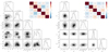 |
Fig. 4. Left panel: corner plot and heat map for the measured best-fit spectral quantities in the case of ℳ = 0.75. The distributions (median, 1st and 3rd quartiles) and the correlations among the measured quantities are shown. The heat map is color-coded and indicates the level of correlations among the same quantities. Right panel: same as left panel, but evaluated using the differences between measured and reference values. |
The lack of any correlation between the spectroscopic measurements and the estimated differences between the same measurements and the input values guarantees the robustness of the outputs of the spectral fitting procedure, in particular against any possible degeneracy in the estimates of the best-fit parameters. This is a non-trivial result because the same emission lines are used to constrain (i) the metal abundance through the equivalent width of the line against the continuum that defines the gas temperature, (ii) the velocity ν from the centroid of the line, (iii) the velocity dispersion w from its broadening. Thus, we can conclude that these measurements are independent from each other at high statistical significance.
4. Structure functions
Most of the information on the kinematics of the ICM can be derived from the analysis of the fluctuations of the velocity and density field. Ideally, the injection/dissipation scale and inertial range should be physically constrained by the 3D power spectrum (e.g., Schuecker et al. 2004; Churazov et al. 2012; Zhuravleva et al. 2012; Gaspari & Churazov 2013); however, it is still possible to derive meaningful pieces of information from their 2D counterparts (e.g., ZuHone et al. 2016). In this work, we only focus on studying the 2D fluctuations of surface brightness, velocity, and velocity dispersion of our simulation set and estimate the accuracy of future X-IFU observations to derive their 2D power spectra.
Following ZuHone et al. (2016), we analyze the structure functions of our X-IFU maps for the quantities of interest, and compare them with those derived from the simulations. For a given physical distance r, the second-order structure function of a given mapped quantity, m(x), is defined as (12)
(12)
The structure function is mathematically related to the autocorrelation function and to the 2D power spectrum, but proves to be particularly useful in our case since it allows us to determine the bias associated with statistical and systematic errors and remove it, provided that these uncertainties are modeled correctly. Specifically, when considering the squared differences of a set of measured quantities in the same distance bin, including errors in the expression we can write![$ \begin{aligned} s_{ij}^{\prime }\,{=}\,[(m_i\,{+}\,\delta m_i) - (m_j\,{+}\,\delta m_j)]^2, \end{aligned} $](/articles/aa/full_html/2018/10/aa33371-18/aa33371-18-eq14.gif) (13)
(13)
being δ
m
i
and δ
m
j
the differences between the measured quantities and the true ones m
i
and m
j
, respectively. By expanding the expression and averaging in the case of symmetric Gaussian errors, σ
tot, it can be shown that (see Appendix C in ZuHone et al. 2016) (14)
(14)
where the symbol ⟨...⟩
r
indicates the average between pairs at the same distance r. The previous expression shows that since both ν and w show an intrinsic variability comparable to that associated with measurement errors (see Table 1), a good model of the latter is necessary to achieve a precise determination of their structure function. However, it should be kept in mind that in real observations σ
tot is not known since it also includes the systematics that are unknown to the observer. To mimic the observational approach we compute the structure function of our observed X-IFU maps by modeling only the effect of statistical errors, which we can estimate from the errors in the fit results. Therefore, we modify Eq. (14) as (15)
(15)
where the last term represents the average of the statistical variance of the set of points at the same distance r. Since in our results we have non-symmetric errors, each value of  is derived from the left-hand and right-hand error as in Eq. (9).
Considering all of the above, we derive the best observational estimate of the (2D) structure functions of surface brightness fluctuations δ, ν, and w, respectively, with the following formulas: (16)
(16)
 (17)
(17)

The quantity δ that appears in Eq. (16) is defined as (19)
(19)
The corresponding statistical error σ δ, stat = σ EM, stat/⟨EM(r)⟩, being ⟨EM(r)⟩ the average surface brightness of the points at the same distance r from the peak of the emission measure map; this conversion allows us to study the surface brightness fluctuations with respect to the average profile. We note that the SF ν (at large r) is tied to the variance of the turbulence field (i.e., specific kinetic energy), while the SF w (line broadening) is linked to the variance of the turbulent velocity, which can be interpreted as a measure of turbulence intermittency.
It is important to note that the region covered by our X-IFU simulations, i.e., the core of our simulated cluster, allows us to estimate fluctuations up to a maximum distance of 350 kpc. In order to obtain a complete representation of the SFs over the full cluster volume (fully capturing the injection scale) we would need to enlarge the total area by a factor of ∼10, with multiple X-IFU pointings, which is beyond the scope of this work. In addition, the SFs measured in the core can significantly vary from the global SFs (which describe the full physical cascade6) because of the cosmic variance and related stochastic nature of the turbulent eddies along a given line of sight. As a reference, we verified that the logarithmic scatter in the amplitude of the SFs due to the different line-of-sight projection in our simulations is Δ A Log ≃ 0.10 − 0.15 (at r < 100 kpc).
The comparison between observationally derived and input SF
δ
, SF
ν
, and SF
w
is shown in Fig. 5. To understand the effect of the statistical error correction, we also show (open circles) the same results neglecting the  terms. The structure function of the emission measure fluctuations δ is recovered almost perfectly, with only a minor difference for the ℳ = 0.5 simulation. This is expected given the high correlation between measured and input quantities (see the discussion in Sect. 3.2) and the small measurement errors. The general shape of the structure function of the velocity field is also recovered, with the three physical models clearly distinguishable. However, measured values show a non-negligible overestimate (about 5–10%); this can be partially explained as systematic errors that are not accounted for in our computation and that would introduce a
  term in the equation. We also point out that the modeling of error subtraction described by Eq. (15) works under the hypothesis of both uniform and Gaussian errors, which is not completely true due to the presence of a non-negligible number of outliers, as discussed in Sect. 3.2. This means that in order to achieve a more robust characterization of SFν, a more accurate error model is required. All these considerations also apply to SFw, with a significantly larger overestimate associated with the error subtraction.
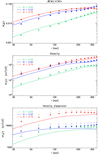 |
Fig. 5. Second-order 2D structure functions of emission measure fluctuations (top panel), velocity (middle panel), and velocity dispersion (bottom panel) as a function of distance for the three ℳ = (0.25, 0.5, 0.75) simulations (green, blue, and red, respectively). In each plot the measured SFs derived from our simulated X-IFU fields (filled dots with error bars) is compared to those of δ, vew, and wew (see definitions in Eqs. (3), (5), and (6)) derived directly from the hydrodynamical simulations in the same field of view (solid lines). Error bars represent the error on the mean computed with 100 bootstrap samplings (in most cases smaller than the dot size). Open circles indicate the values of the measured SFs without the statistical error subtraction (see Eqs. (17) and (18)). The FOV covers only a small fraction of the cluster, namely the core region. |
We analyze the impact of these systematics in determining the properties of the 2D power spectrum, P2D, of the different quantities. As pointed out in ZuHone et al. (2016), if we assume a power-law form of the power spectrum in the inertial range (i.e., below the injection scale), P2D(k) ∝ kα, then the corresponding SF scales as r
γ
, with γ = − (α + 2). Therefore, we fit the SFs of Fig. 5 using (20)
(20)
with r0 fixed to 100 kpc, while A and γ are left as free parameters. We compute the fit in the interval 30–120 kpc to ensure that in all cases we have functions that increase with r and avoid the flattening due to the large-scale plateau. Finally, by comparing the resulting best-fit values obtained from our mock measurements with those obtained directly from the projected simulation quantities, we are able to estimate the impact of the systematics in the structure function on the slope and normalization of the SF itself and, consequently, of their P2D.
We show the results of the fit in Table 2. It is clear that the only significant impact of the systematics in our SFs is in the normalization estimate. The value of Aν, meas exceeds the input value by 15–30%, while for Aw, meas it can be almost doubled. On the other hand, the slopes of the initial structure functions are correctly recovered in all cases, with maximum differences between input and measured values of ∼0.17. This confirms that the systematics in the SFs measurements are induced by an underestimation of the
 , which boosts our measurements but has a minor impact on the slope.
From top to bottom: Normalization and slopes of the structure functions, SF(r), of emission measure fluctuations, velocity, and velocity dispersion, for the three simulations with ℳ = (0.25, 0.5, 0.75) kpc.
5. Summary and conclusions
We have developed, for the first time, an end-to-end mock X-ray analysis pipeline that mimics future Athena X-IFU observations. Our goal was to quantify possible systematics that may arise in the measurements of the main projected physical properties of the ICM, emission measure, temperature, and metallicity; most notably, the two key quantities that will be made available via high-resolution spectroscopic imaging are the line-of-sight velocity ν derived from the centroid shift of the emission lines, and the velocity dispersion w derived from their broadening. In this work we applied our pipeline to a set of three hydrodynamical simulations (Gaspari & Churazov 2013; Gaspari et al. 2014) that model the injection of turbulence in a Coma-like galaxy cluster, assuming different Mach numbers ℳ = (0.25, 0.5, 0.75). Using the SIXTE software, we obtained three simulated event lists that represent X-IFU observations in ideal conditions (i.e., with enough photons not to be limited by statistics) and then applied a realistic observational pipeline to measure and map the quantities mentioned above. This was done by fitting about 600 spectra for each X-IFU FOV, allowing a comparison with the equivalent input projected quantities extracted directly from the hydrodynamical simulations. Finally, we computed the 2D structure functions of the three main quantities that can be used to describe the properties of turbulence, namely emission measure fluctuations ν and w, and verified our ability to recover their input slope and normalization.
Our main results can be summarized as follows:
-
i)
The centroid shift and line broadening measured by fitting the X-IFU spectra correspond well to the emission-weighted velocity and velocity dispersion (see Eqs. (5) and (6), respectively) computed in the same region. The temperature is appropriately described by the spectroscopic-like temperature (Eq. (4), Mazzotta et al. 2004);
-
ii)
No significant bias is found in the measurement of the five physical quantities investigated in our analysis. The expected systematic uncertainties (listed in Table 1) due to the modeling assumed in the fitting procedure are smaller than 5% for all quantities, except for the broadening where it reaches about 15%;
-
iii)
The physical quantities measured with our fitting procedure and their differences with the input projected values prove to be independent from each other at high statistical significance. This corroborates the accuracy of the current spectral fitting approach. Improvements on the fitting errors and to the residual systematic can be considered, for example using optimal binning or other fitting methods;
-
iv)
The overall shape of the 2D structure functions of emission measure fluctuations, velocity, and velocity dispersion is recovered well. However, we observe an excess of 15–30% and of 40–80% in measurement of the normalization of SFν and SFw, respectively: this is due to the limitations of the simplistic assumption on the error shapes;
-
v)
We verified that these discrepancies do not affect the ability to measure the slope of the 2D structure functions of all quantities and thus of their 2D power spectrum. In all cases the input slope is recovered at high precision, with differences smaller than 0.1.
The list of possible failures that may occur in XSPEC during the error computation can be found in https://heasarc.gsfc.nasa.gov/xanadu/xspec/manual/XStclout.html
Acknowledgments
This work has been completed despite the shameful situation of the Italian research system, worsened by an entire decade of severe cuts to the fundings of public universities and research institutes (see, e.g., Abbott 2006, 2016, 2018). This has caused a whole generation of valuable researchers, in all fields, to struggle in poor working conditions with little hope of achieving decent employment contracts and permanent positions, resulting in obvious difficulties in the planning of future research activities, and in open violation of the European Charter for Researchers8. We acknowledge support by the ASI (Italian Space Agency) through Contract no. 2015-046-R.0. M.R. also acknowledges the financial contribution from ASI agreement no. I/023/12/0 “Attività relative alla fase B2/C per la missione Euclid”. M.G. is supported by NASA through Einstein Postdoctoral Fellowship Award Number PF5-160137 issued by the Chandra X-ray Observatory Center, which is operated by the SAO for and on behalf of NASA under contract NAS8-03060. Support for this work was also provided by Chandra GO7-18121X. S.E. acknowledges financial contribution from contracts NARO15 ASI-INAF I/037/12/0, ASI 2015-046-R.0, and ASI-INAF no. 2017-14-H.0. The FLASH code was in part developed by the DOE NNSA-ASC OASCR Flash center at the University of Chicago. HPC resources were in part provided by the NASA HEC Program (SMD-17-7251). E.R. acknowledges the ExaNeSt and Euro Exa projects, funded by the European Union’s Horizon 2020 research and innovation program under grant agreement No. 671553 and No. 754337 and financial contribution from ASI-INAF agreement no. 2017-14-H.0. We thank the anonymous referee for providing useful comments. We are grateful to S. Borgani, K. Dolag, M. Gitti, G. Lanzuisi, and P. Peille for insightful discussions. We also thank the SIXTE development team for their help and support.
References
- Abbott, A. 2006, Nature, 440, 264 [NASA ADS] [CrossRef] [Google Scholar]
- Abbott, A. 2016, Nature, 540, 324 [NASA ADS] [CrossRef] [Google Scholar]
- Abbott, A. 2018, Nature, 554, 411 [NASA ADS] [CrossRef] [Google Scholar]
- Anders, E., & Grevesse, N. 1989, Geochim. Cosmochim. Acta, 53, 197 [Google Scholar]
- Barret, D., Lam Trong, T., den Herder, J.-W., et al. 2016, in Space Telescopes and Instrumentation 2016: Ultraviolet to Gamma Ray, Proc. SPIE, 9905, 99052F [CrossRef] [Google Scholar]
- Beresnyak, A., & Miniati, F. 2016, ApJ, 817, 127 [NASA ADS] [CrossRef] [Google Scholar]
- Biffi, V., Dolag, K., & Böhringer, H. 2013, MNRAS, 428, 1395 [NASA ADS] [CrossRef] [Google Scholar]
- Biffi, V., Borgani, S., Murante, G., et al. 2016, ApJ, 827, 112 [NASA ADS] [CrossRef] [Google Scholar]
- Bonafede, A., Brüggen, M., Rafferty, D., et al. 2018, MNRAS, 478, 2927 [NASA ADS] [CrossRef] [Google Scholar]
- Brunetti, G., Setti, G., Feretti, L., & Giovannini, G. 2001, MNRAS, 320, 365 [NASA ADS] [CrossRef] [Google Scholar]
- Bulbul, G. E., Smith, R. K., Foster, A., et al. 2012, ApJ, 747, 32 [NASA ADS] [CrossRef] [Google Scholar]
- Cappellari, M., & Copin, Y. 2003, MNRAS, 342, 345 [NASA ADS] [CrossRef] [Google Scholar]
- Cho, J., Vishniac, E. T., Beresnyak, A., Lazarian, A., & Ryu, D. 2009, ApJ, 693, 1449 [NASA ADS] [CrossRef] [Google Scholar]
- Churazov, E., Forman, W., Jones, C., Sunyaev, R., & Böhringer, H. 2004, MNRAS, 347, 29 [NASA ADS] [CrossRef] [Google Scholar]
- Churazov, E., Vikhlinin, A., Zhuravleva, I., et al. 2012, MNRAS, 421, 1123 [NASA ADS] [CrossRef] [Google Scholar]
- Croston, J. H., Sanders, J. S., Heinz, S., et al. 2013, ArXiv e-prints [arXiv:1306.2323] [Google Scholar]
- De Grandi, S., Eckert, D., Molendi, S., et al. 2016, A&A, 592, A154 [NASA ADS] [CrossRef] [EDP Sciences] [Google Scholar]
- Dolag, K., Vazza, F., Brunetti, G., & Tormen, G. 2005, MNRAS, 364, 753 [NASA ADS] [CrossRef] [Google Scholar]
- Eckert, D., Roncarelli, M., Ettori, S., et al. 2015, MNRAS, 447, 2198 [NASA ADS] [CrossRef] [Google Scholar]
- Eckert, D., Gaspari, M., Owers, M. S., et al. 2017a, A&A, 605, A25 [NASA ADS] [CrossRef] [EDP Sciences] [Google Scholar]
- Eckert, D., Gaspari, M., Vazza, F., et al. 2017b, ApJ, 843, L29 [NASA ADS] [CrossRef] [Google Scholar]
- Eckert, D., Ghirardini, V., Ettori, S., et al. 2018, A&A, accepted [arXiv:1805.00034] [Google Scholar]
- Ettori, S., Pratt, G.W., de Plaa, J., et al. 2013, ArXiv e-prints [arXiv:1306.2322] [Google Scholar]
- Fisher, R. T., Kadanoff, L. P., Lamb, D. Q., et al. 2008, IBM J. Res. Devel., 52, 127 [CrossRef] [Google Scholar]
- Gaspari, M. 2015, MNRAS, 451, L60 [NASA ADS] [CrossRef] [Google Scholar]
- Gaspari, M., & Churazov, E. 2013, A&A, 559, A78 [NASA ADS] [CrossRef] [EDP Sciences] [Google Scholar]
- Gaspari, M., & Sądowski, A. 2017, ApJ, 837, 149 [NASA ADS] [CrossRef] [Google Scholar]
- Gaspari, M., Churazov, E., Nagai, D., Lau, E. T., & Zhuravleva, I. 2014, A&A, 569, A67 [Google Scholar]
- Gaspari, M., McDonald, M., Hamer, S. L., et al. 2018, ApJ, 854, 167 [NASA ADS] [CrossRef] [Google Scholar]
- Hitomi Collaboration, Aharonian, F., Akamatsu, H., et al. 2016, Nature, 535, 117 [Google Scholar]
- Hitomi Collaboration, Aharonian, F., Akamatsu, H., et al. 2018, PASJ, 70, 9 [NASA ADS] [Google Scholar]
- Hofmann, F., Sanders, J. S., Nandra, K., Clerc, N., & Gaspari, M. 2016, A&A, 585, A130 [NASA ADS] [CrossRef] [EDP Sciences] [Google Scholar]
- Inogamov, N. A., & Sunyaev, R. A. 2003, Astron. Lett., 29, 791 [NASA ADS] [CrossRef] [Google Scholar]
- Khatri, R., & Gaspari, M. 2016, MNRAS, 463, 655 [NASA ADS] [CrossRef] [Google Scholar]
- Lau, E. T., Kravtsov, A. V., & Nagai, D. 2009, ApJ, 705, 1129 [NASA ADS] [CrossRef] [Google Scholar]
- Lau, E. T., Gaspari, M., Nagai, D., & Coppi, P. 2017, ApJ, 849, 54 [NASA ADS] [CrossRef] [Google Scholar]
- Mazzotta, P., Rasia, E., Moscardini, L., & Tormen, G. 2004, MNRAS, 354, 10 [NASA ADS] [CrossRef] [Google Scholar]
- Miniati, F. 2014, ApJ, 782, 21 [NASA ADS] [CrossRef] [Google Scholar]
- Nandra, K., Barret, D., Barcons, X., et al. 2013, ArXiv e-prints [arXiv:1306.2307] [Google Scholar]
- Ogorzalek, A., Zhuravleva, I., Allen, S. W., et al. 2017, MNRAS, 472, 1659 [NASA ADS] [CrossRef] [Google Scholar]
- Petrosian, V. 2001, ApJ, 557, 560 [NASA ADS] [CrossRef] [Google Scholar]
- Piffaretti, R., & Valdarnini, R. 2008, A&A, 491, 71 [NASA ADS] [CrossRef] [EDP Sciences] [Google Scholar]
- Pinto, C., Sanders, J. S., Werner, N., et al. 2015, A&A, 575, A38 [NASA ADS] [CrossRef] [EDP Sciences] [Google Scholar]
- Planelles, S., Fabjan, D., Borgani, S., et al. 2017, MNRAS, 467, 3827 [NASA ADS] [CrossRef] [Google Scholar]
- Pointecouteau, E., Reiprich, T. H., Adami, C., et al. 2013, ArXiv e-prints [arXiv:1306.2319] [Google Scholar]
- Rasia, E., Meneghetti, M., Martino, R., et al. 2012, New J. Phys., 14, 055018 [NASA ADS] [CrossRef] [Google Scholar]
- Roncarelli, M., Ettori, S., Dolag, K., et al. 2006, MNRAS, 373, 1339 [NASA ADS] [CrossRef] [Google Scholar]
- Roncarelli, M., Cappelluti, N., Borgani, S., Branchini, E., & Moscardini, L. 2012, MNRAS, 424, 1012 [NASA ADS] [CrossRef] [Google Scholar]
- Roncarelli, M., Ettori, S., Borgani, S., et al. 2013, MNRAS, 432, 3030 [NASA ADS] [CrossRef] [Google Scholar]
- Sanders, J. S., & Fabian, A. C. 2013, MNRAS, 429, 2727 [NASA ADS] [CrossRef] [Google Scholar]
- Sanders, J. S., Fabian, A. C., Frank, K. A., Peterson, J. R., & Russell, H. R. 2010, MNRAS, 402, 127 [NASA ADS] [CrossRef] [Google Scholar]
- Santos-Lima, R., de Gouveia Dal Pino, E. M., Kowal, G., et al. 2014, ApJ, 781, 84 [NASA ADS] [CrossRef] [Google Scholar]
- Schmid, C., Smith, R., & Wilms, J. 2013, SIMPUT - A File Format for Simulation Input, Tech. report, HEASARC (Cambridge) [Google Scholar]
- Schuecker, P., Finoguenov, A., Miniati, F., Böhringer, H., & Briel, U. G. 2004, A&A, 426, 387 [NASA ADS] [CrossRef] [EDP Sciences] [Google Scholar]
- Shi, X., Komatsu, E., Nagai, D., & Lau, E. T. 2016, MNRAS, 455, 2936 [NASA ADS] [CrossRef] [Google Scholar]
- Smith, R. K., Brickhouse, N. S., Liedahl, D. A., & Raymond, J. C. 2001, ApJ, 556, L91 [NASA ADS] [CrossRef] [Google Scholar]
- Spitzer, L. 1962, Phys. Fully Ion. Gas. (New York: Interscience) [Google Scholar]
- Vazza, F., Brunetti, G., Gheller, C., Brunino, R., & Brüggen, M. 2011a, A&A, 529, A17 [NASA ADS] [CrossRef] [EDP Sciences] [Google Scholar]
- Vazza, F., Roncarelli, M., Ettori, S., & Dolag, K. 2011b, MNRAS, 413, 2305 [NASA ADS] [CrossRef] [Google Scholar]
- Voit, G. M. 2018, ApJ, submitted, [arXiv:1803.06036] [Google Scholar]
- Walker, S. A., Sanders, J. S., & Fabian, A. C. 2015, MNRAS, 453, 3699 [NASA ADS] [Google Scholar]
- Wallis, K. F. 2014, Statist. Sci., 29, 106 [Google Scholar]
- Wilms, J., Brand, T., Barret, D., et al. 2014, in Space Telescopes and Instrumentation 2014: Ultraviolet to Gamma Ray, Proc. SPIE, 9144, 91445X [Google Scholar]
- Zhuravleva, I., Churazov, E., Kravtsov, A., & Sunyaev, R. 2012, MNRAS, 422, 2712 [NASA ADS] [CrossRef] [Google Scholar]
- Zhuravleva, I., Churazov, E., Arévalo, P., et al. 2015, MNRAS, 450, 4184 [Google Scholar]
- ZuHone, J. A., Markevitch, M., & Zhuravleva, I. 2016, ApJ, 817, 110 [NASA ADS] [CrossRef] [MathSciNet] [Google Scholar]
Appendix A: Additional plots
In this Appendix, as a further reference, we show the plot in Fig. 3 for the other two simulations. The plot for the ℳ = 0.25 and ℳ = 0.5 simulations are shown in Fig. A.1 and Fig. A.2, respectively.
Appendix B: Statistical uncertainty with asymmetric errors
The calculation of the expected variance of the difference between true and measured quantities in the case of asymmetric errors must take into account the properties of the split-normal (or double Gaussian) distribution (see, e.g., Wallis 2014). Specifically, we consider that for a given measurement  the posterior probability of the true value X is described by the distribution
![$ \begin{aligned} f(X)\,{=}\,\left\{ \begin{array}{l} A \, \exp {\left[-\frac{(X-\mu )^2}{2\sigma _1^2}\right]} \ \ \ \mathrm{for } \ X\,{\le }\,\mu \\ A \, \exp {\left[-\frac{(X-\mu )^2}{2\sigma _2^2}\right]} \ \ \ \mathrm{for } \ X\,{\ge }\,\mu \, \end{array}, \right. \end{aligned} $](/articles/aa/full_html/2018/10/aa33371-18/aa33371-18-eq27.gif) (B.1)
(B.1)
where  . In this case μ represents the mode of the distribution, i.e., the nominal value of the measurement. It is possible to show that the mean and the variance of the distributions are
 (B.2)
(B.2)
respectively. Since we are interested in the expected dispersion with respect to μ, which we consider as our reference value for the measurements, we can derive it from the last two equations,![$ \begin{aligned} \sigma _{\mu }^2(X)\,{=}\,V(X)\,{+}\,[E(X)-\mu ]^2\,{=}\,\left(\sigma _2-\sigma _1\right)^2\,{+}\,\sigma _1 \sigma _2, \end{aligned} $](/articles/aa/full_html/2018/10/aa33371-18/aa33371-18-eq31.gif) (B.4)
which we adopt as a definition of
(B.4)
which we adopt as a definition of  in Eq. (9).
All Tables
Statistical estimates for the accuracy on the measurements of the five physical quantities compared to the input values in the three simulations.
From top to bottom: Normalization and slopes of the structure functions, SF(r), of emission measure fluctuations, velocity, and velocity dispersion, for the three simulations with ℳ = (0.25, 0.5, 0.75) kpc.
All Figures
|
Fig. 1. Example of a mock X-IFU spectrum extracted from the ℳ = 0.75 run and of its fitting procedure. Top panel: spectral data points with error bars (black crosses) in the whole fitting interval and best-fit model (blue line). Fit results, with errors, for the five free parameters are indicated in the box in the bottom left. The value of ν is obtained assuming the true redshift, z 0 = 0.1, is known. The bottom subpanel shows the residuals with respect to the model. Bottom panel: same as top panel, but zooming on the 6–6.4 keV energy range (highlighted in yellow in the top panel) where the most prominent emission lines are present. In this case the features correspond to the blending of the Fe XXV and Fe XXVI K complexes. In both panels data points have been rebinned for display purposes. The plot scaling for the spectra is logarithmic in the top panel and linear in the bottom panel. |
| In the text | |
|
Fig. 2. X-IFU maps showing input quantities (top panels) vs. measured ones (bottom) for the ℳ = 0.75 model. Input quantities are derived directly from the simulation output, considering the average along the line of sight enclosed by the X-IFU pixel (4.38 arcsec wide) and computed with the definitions in Eqs. (3)–(6). For measured quantities we show the nominal value derived from the fitting of our synthetic spectra (see text for details) in the corresponding 588 Voronoi regions (≈125 arcsec2 each). From left to right: emission measure, gas temperature (spectroscopic-like, in the top panel), velocity, and velocity dispersion (both emission-weighted, in the top panels). |
| In the text | |
|
Fig. 3. Scatter plots of observed quantities with errors (y-axis) vs. input projected values (x-axis) for the ℳ = 0.75 simulation. Top left: emission measure. Top right: temperature vs. spectroscopic-like temperature. Bottom left: velocity vs. emission-weighted velocity. Bottom right: velocity dispersion vs. emission-weighted velocity dispersion. In each plot the red solid lines shows the identity and the bottom panel shows the residuals in units of σ. In the top left corner of each panel we show the Spearman correlation rank between observed and input values. |
| In the text | |
|
Fig. 4. Left panel: corner plot and heat map for the measured best-fit spectral quantities in the case of ℳ = 0.75. The distributions (median, 1st and 3rd quartiles) and the correlations among the measured quantities are shown. The heat map is color-coded and indicates the level of correlations among the same quantities. Right panel: same as left panel, but evaluated using the differences between measured and reference values. |
| In the text | |
|
Fig. 5. Second-order 2D structure functions of emission measure fluctuations (top panel), velocity (middle panel), and velocity dispersion (bottom panel) as a function of distance for the three ℳ = (0.25, 0.5, 0.75) simulations (green, blue, and red, respectively). In each plot the measured SFs derived from our simulated X-IFU fields (filled dots with error bars) is compared to those of δ, vew, and wew (see definitions in Eqs. (3), (5), and (6)) derived directly from the hydrodynamical simulations in the same field of view (solid lines). Error bars represent the error on the mean computed with 100 bootstrap samplings (in most cases smaller than the dot size). Open circles indicate the values of the measured SFs without the statistical error subtraction (see Eqs. (17) and (18)). The FOV covers only a small fraction of the cluster, namely the core region. |
| In the text | |
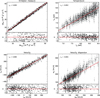 |
Fig. A.1. Same as Fig. 3, but for the ℳ = 0.25 simulation. |
| In the text | |
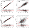 |
Fig. A2. Same as Fig. 3, but for the ℳ = 0.5 simulation. |
| In the text | |
Current usage metrics show cumulative count of Article Views (full-text article views including HTML views, PDF and ePub downloads, according to the available data) and Abstracts Views on Vision4Press platform.
Data correspond to usage on the plateform after 2015. The current usage metrics is available 48-96 hours after online publication and is updated daily on week days.
Initial download of the metrics may take a while.