| Issue |
A&A
Volume 618, October 2018
|
|
|---|---|---|
| Article Number | A10 | |
| Number of page(s) | 13 | |
| Section | Stellar structure and evolution | |
| DOI | https://doi.org/10.1051/0004-6361/201833361 | |
| Published online | 03 October 2018 | |
Impacts of radiative accelerations on solar-like oscillating main-sequence stars
1 LESIA, Observatoire de Paris, PSL Research University, CNRS, Université Pierre et Marie Curie, Université Paris Diderot, 92195 Meudon, France
e-mail: This email address is being protected from spambots. You need JavaScript enabled to view it.
2 LUTH, Observatoire de Paris, PSL Research University, CNRS, Université Pierre et Marie Curie, Université Paris Diderot, 92195 Meudon, France
3 Institut de Physique de Rennes, Université de Rennes 1, CNRS UMR 6251, 35042 Rennes, France
4 Institut d’Astrophysique Spatiale, UMR8617, CNRS, Université Paris XI, Bâtiment 121, 91405 Orsay Cedex, France
5 Département de Physique et d’Astronomie, Université de Moncton, Moncton, N.B. E1A 3E9, Canada
6 Université de Nice Sophia-Antipolis, OCA, Laboratoire Lagrange CNRS, BP 4229, 06304 Nice Cedex, France
Received:
4
May
2018
Accepted:
26
June
2018
Abstract
Context. Chemical element transport processes are among the crucial physical processes needed for precise stellar modelling. Atomic diffusion by gravitational settling is usually taken into account, and is essential for helioseismic studies. On the other hand, radiative accelerations are rarely accounted for, act differently on the various chemical elements, and can strongly counteract gravity in some stellar mass domains. The resulting variations in the abundance profiles may significantly affect the structure of the star.
Aims. The aim of this study is to determine whether radiative accelerations impact the structure of solar-like oscillating main-sequence stars observed by asteroseismic space missions.
Methods. We implemented the calculation of radiative accelerations operating on C, N, O, Ne, Na, Mg, Al, Si, S, Ca, and Fe in the CESTAM code using the single-valued parameter method. We built and compared several grids of stellar models including gravitational settling, some with and others without radiative accelerations. We considered masses in the range [0.9, 1.5] M⊙ and three values of the metallicity around the solar value. For each metallicity we determined the mass range where differences between models due to radiative accelerations exceed the uncertainties of global seismic parameters of the Kepler Legacy sample or expected for PLATO observations.
Results. We found that radiative accelerations may not be neglected for stellar masses higher than 1.1 M⊙ at solar metallicity. The difference in age due to their inclusion in models can reach 9% for the more massive stars of our grids. We estimated that the percentage of the PLATO core program stars whose modelling would require radiative accelerations ranges between 33% and 58% depending on the precision of the seismic data.
Conclusions. We conclude that in the context of Kepler, TESS, and PLATO missions which provide (or will provide) high-quality seismic data, radiative accelerations can have a significant effect when properly inferring the properties of solar-like oscillators. This is particularly important for age inferences. However, the net effect for each individual star results from the competition between atomic diffusion including radiative accelerations and other internal transport processes. Rotationally induced transport processes for instance are believed to reduce the effects of atomic diffusion. This will be investigated in a forthcoming companion paper.
Key words: diffusion / stars: abundances / stars: evolution / stars: interiors / asteroseismology / stars: solar-type
© ESO 2018
 Open Access article, published by EDP Sciences, under the terms of the Creative Commons Attribution License (http://creativecommons.org/licenses/by/4.0), which permits unrestricted use, distribution, and reproduction in any medium, provided the original work is properly cited.
1. Introduction
Understanding and modelling the transport of chemical elements inside stars still remain difficult challenges for the theory of stellar structure and evolution. Chemical abundances play an important role in determining the structure and evolution of stars. The internal distribution of chemical elements results from the competition of several transport processes within the star which are still barely understood and/or poorly modelled.
Transport processes can be constrained using photospheric observations, but the impact on the internal structure can only be probed using stellar oscillations. The CoRoT (Baglin et al. 2013) and Kepler (Gilliland et al. 2010) space missions provided a wealth of high-quality photometric light curves. Seismic data derived from these observations improved the characterisation of the observed main-sequence stars and provide constraints on their internal structures (for reviews, see Chaplin et al. 2013; Deheuvels et al. 2016; Christensen-Dalsgaard 2016).
The PLATO ESA mission (Rauer et al. 2014) will be launched in 2026 and offers a new perspective to constrain our stellar evolution models further. The objectives of the project are the detection and the full characterisation of Earth-like planets orbiting solar-like stars, and the study of the evolution of star-planet systems. While the detection of exoplanets requires very high signal-to-noise ratios and long observing times, the full characterisation of these detected objects requires the precise determination of the stellar parameters of the host-stars. The aim of the PLATO mission is to observe a large number of stars while combining two techniques:
the detection by photometric transit and a ground-based follow up in radial velocity which will provide the planet-to-host star radius and mass ratios, respectively;
asteroseismology analysis (coupled with spectroscopic observations) which will provide precise masses, radii, and more importantly ages of the host stars.
The goal is to reach uncertainties of the order of or less than 3% in radius and 10% in mass for the planets. This translates into the need to reach uncertainties of the order of or less than 2% in radius and 15% in mass for the host-stars. A PLATO objective is also to reach an uncertainty as small as 10% for the age determination of a solar-like host-star. The current stellar models are still not able to provide such accuracy.
The study of the competition between microscopic and macroscopic transport processes is a necessary step towards more accurate stellar models. Helioseismology showed the necessity of including atomic diffusion to properly model the Sun (Christensen-Dalsgaard et al. 1993). It is a microscopic process which occurs in every star due to the gradients of T, P, etc. This process was first discussed by Eddington (1926) and the importance of radiative accelerations was first recognised by Michaud (1970) and Watson (1971). The diffusion velocity of an element mainly depends on two forces (or accelerations): gravity, which makes the element migrate toward the centre of the star, and radiative accelerations, which generally push the element up toward the surface. The latter is due to the capability of ions to absorb photons (according to their atomic properties) and to acquire part of their momentum. Atomic diffusion principally results from the competition between these two forces.
For G-, F-, and late A-type main-sequence stars (Population I and II), models including atomic diffusion may produce depletions or accumulations of chemical elements that are too large if no additional mixing other than convection is considered. This is the reason why models need to include additional macroscopic transport processes to reproduce the observed surface abundances (e.g. Korn et al. 2007). Atomic diffusion can then be used as a proxy to determine the efficiency of macroscopic transport processes or the rate of mass loss needed to reproduce observations and then predict which processes play a role (e.g. Talon et al. 2006; Michaud et al. 2004, 2011).
Atomic diffusion leads to local modifications of the abundance profiles, and thus to a modification of the Rosseland opacities. This has important structural effects in stars, for example the opacity-induced iron and nickel convection zone triggered by the local accumulation of these species around 200 000 K and where these elements are the main contributors to the opacity in F- and A-type stars (Richard et al. 2001; Théado et al. 2009; Deal et al. 2016). This opacity modification close to the bottom of the surface convection zone also causes an increase of the mass of the surface convection zone in F-type stars (Turcotte et al. 1998a). The local accumulation of elements may also lead to an inverse mean molecular weight gradient which triggers thermohaline (or fingering) convection in F- and A-type stars (Théado et al. 2009; Deal et al. 2016) and in B-type stars (Hui-Bon-Hoa & Vauclair 2018). It was shown that neglecting radiative accelerations in the modelling of 94 Ceti A (an F-type star showing solar-like oscillations) using asteroseismic data leads to a 4% age difference (Deal et al. 2017).
Currently only a few evolution codes incorporate consistent computations of stellar models including the complete treatment of atomic diffusion. The Montreal/Montpellier code (Turcotte et al. 1998b) computes radiative accelerations using OPAL monochromatic data and the opacity sampling method (e.g. LeBlanc et al. 2000). The Toulouse Geneva Evolution Code (Hui-Bon-Hoa 2008; Théado et al. 2012) includes the OPCD package1 from the Opacity Project calculations (Seaton 2005) for the opacities and computes radiative accelerations using the single-valued parameter (SVP) approximation proposed by Alecian & LeBlanc (2002) and LeBlanc & Alecian (2004). The SVP approximation allows very fast computations with no need for monochromatic data as they are tabulated within the method. The MESA code computes Rosseland mean opacities and radiative accelerations with the OPCD3 method (Paxton et al. 2018) optimised by the work of Hu et al. (2011). In the present paper, we add to the above list the CESTAM code (Marques et al. 2013) where we implemented the radiative accelerations within the framework of the SVP approximation while using the OPCD3 package for calculations of opacities.
Atomic diffusion has an important impact on the structure of stars. The effects are detectable in the Sun. It has also been shown to play a role in several other types of pulsating stars (Charpinet et al. 1997; Turcotte et al. 2000; Alecian et al. 2009; Théado 2012). Our aim here is to determine whether atomic diffusion, including the effect of radiative accelerations, needs to be taken into account in the modelling of solar-like oscillating main-sequence stars. This is a prerequisite for an optimal interpretation of the data provided by CoRoT and Kepler and by future space missions such as TESS and PLATO. Macroscopic transport processes such as those induced by turbulent convection and/or rotation also play an important role, and the competition with atomic diffusion is not straightforward; several parameters come into play and the net result likely depends on the type of stars, if not on the specificities of each individual star. We have therefore started an in-depth study which should ultimately provide the net result of this competition on the transport of chemical elements and the associated consequences on the structure, the evolution of the star, and its solar-like oscillating properties. The present paper is the first step of this study. Our purpose here is a theoretical quantification of the sole impact of atomic diffusion – more specifically the radiative acceleration process – on the structure, surface abundances, and some basic seismic properties of stars. No macroscopic processes other than convection are taken into account. The results presented here may then be interpreted as the maximum impact of atomic diffusion including radiative accelerations. The inclusion of the competitive effect of rotationally induced mixing as allowed by our evolutionary code is in progress and will constitute the second paper of the series.
The paper is organised as follows: we first detail the new developments of the CESTAM code in Sect. 2. Section 3 then presents the grids of stellar models which focus on low-mass main-sequence stars and the impact of the radiative accelerations on the stellar structure and chemical abundances by comparing models computed with and without radiative accelerations. Some seismic implications are presented in Sect. 4. The impact of the radiative acceleration on the surface iron abundance and thereby on the stellar characterisation are discussed in Sect. 5, while Sects. 6 and 7 are devoted to discussions and conclusions, respectively.
2. CESTAM stellar models
2.1. Standard physics
The stellar models are computed using the CESTAM code (Marques et al. 2013); it is based on the CESAM code (Morel 1997; Morel & Lebreton 2008), and it has a more detailed treatment of rotationally induced transport processes. Here we do not consider the effect of rotation. A second forthcoming paper will discuss the net results of the competition between atomic diffusion (including radiative accelerations) and rotationally induced transport of angular momentum and chemical elements.
The CESTAM models can be computed using the opacities given by the OP (Seaton 2005) or OPAL (Iglesias & Rogers 1996) tables complemented at low temperature by the Wichita opacity data (Ferguson et al. 2005). The equation of state used is OPAL2005 (Rogers & Nayfonov 2002). The nuclear reactions are taken from the NACRE compilation (Angulo 1999) except for the 14N(p,γ)15O reaction, for which we used the LUNA reaction rate given in Imbriani et al. (2004). The convection was treated following (Canuto et al. 1996; hereafter CGM) with a mixing-length l = αCGMHP, where HP is the pressure scale height. We took into account the overshooting of the convective core, with an overshoot extent of 0.15 × min(HP, rcc), where rcc is the radius of the Schwarzschild convective core. This choice is compatible with recent determinations of the overshooting extent based on the study of eclipsing binaries (Claret & Torres 2016) and on asteroseismology of solar-type stars (Deheuvels et al. 2015). The atmosphere is computed in the grey approximation and integrated up to an optical depth of τ = 10−4 with no mass loss taken into account. We used the solar mixture of Asplund et al. (2009) with meteoritic abundances for refractory elements as recommended by Serenelli (2010).
In CESTAM two formulations are available for atomic diffusion: the first is based on the work of (Michaud & Proffitt 1993; hereafter MP93) and the second on the Burgers equations (Burgers 1969). Here we used the MP93 formulation. The MP93 approximation used in the CESTAM code considers the diffusion of trace elements (with partial ionisation) in a fully ionised plasma of H and He. This is an approximation of the Burgers equations. Some comparisons were made with the full Burgers treatment for the Sun (Turcotte et al. 1998b), and in the framework of the Evolution and Seismic Tool Activity (ESTA) for the CoRoT mission for the effect of gravitational settling only (Thoul et al. 2007; Montalbán et al. 2007; Lebreton et al. 2008). The advantage of the MP93 method is that computational times are very short.
2.2. Partial ionisation
Partial ionisation, which is often not considered in evolution codes, is extremely important for atomic diffusion calculations (Montmerle & Michaud 1976; Michaud et al. 2015), firstly because radiative acceleration depends on atomic properties of ions, and secondly because the diffusion velocity is proportional to the diffusion coefficient (Dip), which is proportional to  (where Zi is the electric charge of the ion in proton charge units). Hence, for instance, for two ions with respective charges Zi of 5 and 6 undergoing the same resultant acceleration in the same stellar layer, the velocity of the ion with charge 6 is 30% lower than that of the ion with charge 5. Another example: assuming that iron is fully ionised in diffusion velocity calculations around the depth where the iron opacity bump occurs (log T ≈ 5.2) gives erroneous velocity estimation by more than a factor of 10. The error made by assuming full ionisation in atomic diffusion velocity calculations is larger for stars with a small surface convection zone (larger Teff) since ions have lower Zi at its bottom (cooler layers). Therefore, neglecting partial ionisation in diffusion calculations of chemical elements leads to large underestimates of the diffusion velocities. In this study, partial ionisation on heavy elements is taken into account through an average electric charge
  (instead of Zi) for each element. This significantly simplifies the numerical treatment of the diffusion equations (see Sect. 2.3) since individual ions do not need to be considered (the same approximation is used in Turcotte et al. 1998b). Hereafter, i represents an element whose atoms locally possess an average electric charge
  depending on the local plasma conditions.
2.3. Diffusion equation
The equation describing the evolution of the chemical composition reads
![Mathematical equation: $\rho {{\partial {c_i}} \over {\partial t}} = - {1 \over {{r^2}}}{\partial \over {\partial r}}\left[ {{r^2}\rho {D_{{\rm{turb}}}}{{\partial {c_i}} \over {\partial r}}} \right] - {1 \over {{r^2}}}{\partial \over {\partial r}}[{r^2}\rho {v_i}{c_i}] - {\lambda _i}{c_i},$](/articles/aa/full_html/2018/10/aa33361-18/aa33361-18-eq4.gif) (1)
(1)
where ci is the concentration of element i, ρ is the density in the considered layer, Dturb is a turbulent diffusion coefficient, and λi is the nuclear reaction rate related to the element i. In Eq. (1), vi is the atomic diffusion velocity that can be expressed in the case of a trace element i as
![Mathematical equation: ${v_i} = {D_{ip}}\left[ { - {{\partial \ln {c_i}} \over {\partial r}} + {{{A_i}{m_{\rm{P}}}} \over {kT}}({g_{{\rm{rad}},i}} - g) + {{({{\bar Z}_i} + 1){m_{\rm{P}}}g} \over {2kT}} + {\kappa _T}{{\partial {\rm{ln}}T} \over {\partial r}}} \right],$](/articles/aa/full_html/2018/10/aa33361-18/aa33361-18-eq5.gif) (2)
(2)
where Dip is the diffusion coefficient of element i relative to protons, and Ai is its atomic mass. The variable grad,i is the radiative acceleration on element i, g is the local gravity,  is the average charge (in proton charge units) of element i (roughly equal to the charge of the “dominant ion”), mP is the mass of a proton, k is the Boltzmann constant, T is the temperature, and κT is the thermal diffusivity. It should be noted that
  is used when estimating Dip.
The competition between macroscopic transport processes and atomic diffusion is given by the first two terms on the right-hand side of Eq. (1).
2.4. Radiative accelerations in CESTAM
2.4.1. Atomic diffusion
In some evolution codes including atomic diffusion, a mixture of hydrogen, helium, and of a mean heavy element with respective mass fractions X, Y, and Z are considered (e.g. Thoul et al. 1994). This (X, Y, Z) mixture treatment of atomic diffusion gives acceptable results (depending on the needed accuracy) for stars with masses close to that of the Sun, i.e. in stars where radiative accelerations are systematically weak compared to gravity (i.e. gravitational settling is dominant). However, this approximation is no longer valid for more massive stars where radiative accelerations dominate gravity. In this case, the migration of chemical elements is often towards the surface, depending on the interaction of their ions with the radiation flux. The sign and intensity of the diffusion velocity of a given species depends on the atomic properties of the dominating ions, and on depth (or local physical conditions). This is why elements cannot be treated as a unique mean heavy element Z.
In its present version, CESTAM computes the evolution of abundances of all the elements available in the OPCD3 package (Seaton 2005) and of some isotopes: H, 3He, 4He, 12C, 13C, 14N, 15N, 15O, 16O, 17O, 22Ne, 23Na, 24Mg, 27Al, 28Si, 31P (without radiative accelerations), 32S, 40Ca, and 56Fe. It also takes into account the partial ionisation in computing diffusion velocities (see Eq. (2)), which is a major new development in the evolution code under consideration. It is shown in the next sections that modifications of the structure and surface abundances of stars occur when  is used instead of the charge of the fully ionised element.
Radiative accelerations in CESTAM are computed using the SVP approximations proposed by Alecian & LeBlanc (2002) and LeBlanc & Alecian (2004). There are mainly three and this is one of them (see Alecian 2018): (i) direct use of atomic data (the most accurate method, but the most computationally expensive to carry out), (ii) use of opacity tables with fixed frequency grids (less accurate, but numerically lighter), (iii) use of parametric approximations (less accurate than (ii), but numerically extremely fast). The first method is generally used to compute radiative accelerations in stellar atmospheres (Hui-Bon-Hoa et al. 2000; Alecian & Stift 2004, 2006; LeBlanc et al. 2009) and necessitates direct integration over atomic transition profiles. The second is valid for stellar interiors and is used in the Montreal/Montpellier code, and is also employed (with interpolation techniques) in the OPCD3 package (Seaton 1997, 2007). The third method corresponds to the SVP approximations and is only valid for stellar interiors.
The SVP method is based on a simplified form of the equations for radiative accelerations. They are obtained by separating the terms involving the atomic quantities from those describing the local plasma. The SVP method needs very small tables, contrarily to the other methods. These small tables, which only provide six parameters per ion, are pre-calculated for various stellar masses, and the numerical routines have to interpolate these data to fit the mass of the considered star (some tables can be found on the website2, and a larger set of tables is in preparation). This method is numerically efficient and is tailored for use in stellar evolution codes.
The SVP method was implemented in the TGEC code (Théado et al. 2012), and we proceeded in the same way for its implementation in CESTAM using the same set of tabulated parameters as for TGEC. In this study, radiative accelerations are computed for C, N, O, Ne, Na, Mg, Al, Si, S, Ca, and Fe. The SVP parameters have been calculated with the use of the Opacity Project data (Seaton 1992; Cunto et al. 1993).
In order to avoid numerical instabilities due to sharp gradients of abundance produced by radiative accelerations, we added an ad hoc turbulent mixing coefficient, as done by Théado et al. (2009) and Deal et al. (2016). The turbulent coefficient is expressed as
 (3)
(3)
where Dbcz and rbcz are the value of Dmix and the value of the radius at the bottom of the convection zone, respectively. For the grids we chose Dbcz,1 = 500 cm2 s−1 and Δ1 = 0.02 of the radius of the star and Dbcz,2 = 200 cm2 s−1 and Δ2 = 0.1. This turbulent mixing coefficient was chosen so as not to affect significantly the evolution of the star, and it has a negligible effect on the results presented below.
2.4.2. Opacity tables
In our models, atomic diffusion notably modifies the initial mixture of heavy elements in the outer layers, which implies that pre-computed Rosseland opacity tables cannot be used throughout the interior and all along the evolution. We therefore had to recompute the Rosseland mean opacity locally at each timestep in the layers where the mixture changes considerably. For this purpose, we implemented in CESTAM a dedicated routine (mx.f) which handles the monochromatic opacity tables from the OPCD3 package (Seaton 2005).
Since running the mx.f routine is time-consuming, we recomputed the Rosseland opacity only in the outer layers, when log(T ) < ≈6.23. We note the following:
at higher temperatures, to save computing time, we used the pre-computed Rosseland mean OP opacity tables described in Sect. 2.1.
at low temperatures (T < 104 K) the OPCD3 opacities are still available. Therefore, for consistency, we preferred to use them rather than the more complete Wichita tables (which provide Rosseland means including molecular lines for a given mixture, but are not available in the form of monochomatic opacities). The impact of using OPCD instead of Wichita opacities in the low-temperature domain is that we miss the molecular contribution to the opacity. This may have some impact on the stellar properties especially for the colder stars. However, for these stars radiative accelerations are negligible and since our goal is to perform a relative comparison, this should not significantly modify our conclusions.
2.5. Comparison and validation of the implementations
To verify the validity of the new developments presented in Sect. 2.4, we compared the results obtained with our new version of CESTAM to those obtained with the Montreal/Montpellier code. We chose a model of 1.4 M⊙ with parameters listed in Table 1. Since the input physics of the models is not exactly the same (especially the equation of state and opacity tables) the structures are slightly different, but close enough for our purpose.
Initial parameters of the comparison model.
Figure 1 shows the abundance profiles of various elements. The agreement between the two codes is very satisfactory. The differences between them never exceed 3% for the surface abundances. Elements are depleted or accumulated in the same way. We have also compared models for more massive stars, and the agreement is at the same level. We are therefore confident in the use of this new version of the CESTAM code.
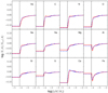 |
Fig. 1. Comparisons of abundance profiles for different elements according to log(ΔM/M*) (where ΔM is the mass between the considered layer and the surface) for a 1.4 M⊙ at Z = 0.025 and 400 Myr between a model computed with the Montreal/Montpellier code (blue dashed curves) and the CESTAM code (red solid curves). The solid vertical lines indicate the position of the bottom of the surface convection zone of the models. |
3. Effects of atomic diffusion on the internal structure
Our goal here is to evaluate the range of stellar mass and initial chemical composition for which radiative accelerations (hereafter grad) cannot be neglected when computing accurately the structure and evolution of solar-like oscillating main-sequence stars. This will allow us to determine masses above which grad has to be taken into account to properly infer stellar parameters (age, mass, radius) from models. These are lower-limit masses because macroscopic transport processes (apart from convection) are not taken into account. This will allow us to save computational time when their effects are negligible. For that purpose we built two sets of stellar model grids described below.
3.1. Our grids of models
We first define three grids of models listed in Table 2, each of them corresponding to a different metallicity. We have chosen masses in the range [0.9, 1.5] M⊙, a range for which grad is expected to have the most significant impact on the structure and evolution of solar-like oscillating main-sequence stars. In order to cover the wide range of metallicities of the CoRoT, Kepler, and the future TESS and PLATO targets, we have considered three values of the initial metallicity for grids 1–3, respectively [Fe/H]ini = −0.35, +0.035, and +0.25 dex, with
![Mathematical equation: ${\rm{[Fe/H]}} = {\rm{log}}\left( {{X_{{\rm{Fe}}}}/{X_{\rm{H}}}} \right) - {\rm{log}}{\left( {{X_{{\rm{Fe}}}}/{X_{\rm{H}}}} \right)_ \odot },$](/articles/aa/full_html/2018/10/aa33361-18/aa33361-18-eq10.gif) (4)
(4)
Characteristics of the grids of models.
where XH and XFe are the hydrogen and iron abundances in mass fraction. Models cover the whole main-sequence lifetime up to the stage where the central hydrogen content is XC = 0.05.
For each of these three grids, we have computed a first set of models including grad, and a second set without grad (gravitational settling only) including convection as the only macroscopic transport process. The values of the mixing-length parameter αCGM and initial helium abundance Yini at solar metallicity were inferred from a solar model calibration. As grad is negligible in the Sun the calibration was done with gravitational settling only. A solar calibration consists in adjusting the initial helium abundance Yini,⊙, metallicity (Z/X)ini,⊙, and αCGM of a 1 M⊙ model so that at solar age it reaches the observed solar luminosity, radius, and photospheric metallicity (see Morel & Lebreton 2008). We obtained Yini,⊙ = 0.2578 and αCGM = 0.68. From Yini,⊙ and a primordial helium abundance YBB = 0.247 (Peimbert et al. 2007), we obtained a helium-to-metal enrichment ratio ΔY/ΔZ = (Yini,⊙ − YBB)/Zini,⊙ = 0.9, which we used to get the initial helium abundance for models with other metallicities.
3.2. Evolutionary tracks
To characterise the differences between models with and without grad in the abundances and the structure of stellar interiors, we computed evolutionary tracks presented in Fig. 2 for the three grids of models described in Table 2. Atomic diffusion processes are rather efficient in the outer layers of stars because diffusion timescales are approximately proportional to the density of protons. For a given star, there is always a layer beyond which the diffusion timescale is greater than the age of the considered star. If this limit layer is too close to (or above) the bottom of the outer convection zone, there is not enough time for atomic diffusion to play a significant role during the lifetime of the star. This is why the effects of atomic diffusion at solar metallicity are greater for stars with solar mass (Turcotte et al. 1998b) or greater, i.e. for stars with a superficial convection zone that is not deeper than that of the Sun. However, it should be noted that significant effects for lower mass stars cannot be excluded since the age of these stars may be old enough (see Dotter et al. 2017). Moreover, since at low metallicities, surface convective zones are shallower, atomic diffusion may therefore be efficient for lower masses (Richard et al. 2002).
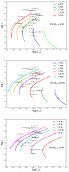 |
Fig. 2. HR diagrams for initial [Fe/H]ini = −0.35 (top panel), [Fe/H]ini = 0.035 (middle panel), and [Fe/H]ini = +0.25 (lower panel). The dashed curves represent models without grad and the solid curves represent models including grad. Black symbols are stars from the Kepler Legacy sample (Lund et al. 2017; Silva Aguirre et al. 2017). |
In Fig. 2 the evolutionary tracks are shown for several initial metallicities (i.e. representative of the photosphere when abundances are still homogeneous outside the stellar core) and for masses ranging from 0.9 to 1.5 M⊙. For the lowest metallicity ([Fe/H]ini = −0.35) the role of grad is evident for masses higher than 1.1 M⊙. This lower mass threshold is 1.3 M⊙ for [Fe/H]ini = 0.035, and 1.45 M⊙ for [Fe/H]ini = +0.25. The role of grad is stronger at low metallicity because grad values are higher for lower abundances. This is a radiation transfer effect since the momentum transfer between the net radiation flux and the considered element is strongly dependent on the saturation effect of bound-bound atomic transitions (Alecian & LeBlanc 2000).
3.3. Abundance variations
Competition between gravity and grad leads to a migration of the chemical elements inside stable zones (when no mixing is at work) of the stars. When grad is not taken into account, all the elements (except hydrogen) migrate toward the centre of the star due to gravitational settling, and this may cause strong depletion of metals at the surface. Therefore, taking into account grad generally prevents this abnormal superficial depletion (see Ne, Mg, and Ca in Fig. 3). In some cases grad is so high at the bottom of the surface convection zone, that metals enter the convection zone and their superficial abundances increase (see Al and Fe in Fig. 3 for the 1.4 M⊙ case).
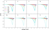 |
Fig. 3. Evolution of surface abundances ([X/H] calculated as in Eq. 4) with time for the eight elements in grid 2 at solar metallicity. The solid and dashed curves respectively represent models with and without grad. |
These changes in element distribution inside the star, iron in particular, explain the slightly different evolution of the models in Fig. 2. This shows that [Fe/H], an observable parameter characterising stars, may be affected by the inclusion of grad. When [Fe/H] is used as an observational constraint in stellar evolution calculation to determine unknown stellar parameters like age or mass, the error in that determination will likely be larger if the grid is computed without the effect of grad (see Sect. 5). In our three grids, the difference in [Fe/H] goes from 0 to 1.7 dex (see Fig. 4) between the models with and without grad. As discussed previously, the effect of grad for the largest metallicity grid (grid 3) is lower than for the others, and it is visible in the difference in [Fe/H]. Despite this, the difference in [Fe/H] is larger for the model with 1.4 M⊙ of grid 2 than for the model with 1.2 M⊙ of grid 1 even if grad is more efficient for the models of grid 1. This is due to the deepening of the surface convection zone, which is larger at low metallicity and dilutes the accumulated iron more efficiently in the surface convective zone (see Sect. 3.4).
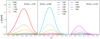 |
Fig. 4. Evolution of the difference in [Fe/H] between models with and without grad for the three grids of models. XC is the central hydrogen mass fraction. The solid lines show the differences for models including the effect of partial ionisation, while the dashed lines show the differences when this process is not taken into account. |
The surface abundances of some elements (He, C, N, and O for instance) in our computations are not representative of the values obtained from the observations of G- and F-type stars (at least during a fraction of the evolution of the models). The maximum depletion observed for these elements is ≈0.4dex for star with a solar metallicity (see Adibekyan et al. 2012; Bensby et al. 2014; Brewer et al. 2016). These elements are not supported (or only weakly) by radiative accelerations and are largely depleted in the models even when grad is taken into account. This result is expected because these models do not include additional mixing processes (e.g. induced by rotation) which should reduce these large depletions. The abundances of the present study can then be considered as upper limits of what can be obtained from more complete models including atomic diffusion and competing macroscopic processes.
3.4. Position of the bottom of the surface convection zone
In the mass range covered by our model sample, the main abundance differences between the two sets of models occur inside the convection zones due to the diffusion flux of iron at their bottom. There is no significant accumulation of metals in layers below the surface convection zone where atomic diffusion processes are too slow to produce abundance stratifications, contrarily to what happens in A- and B-type stars (Richard et al. 2001; Théado et al. 2009; Deal et al. 2016). Here the structure of the models is modified only near the stellar surface.
The accumulation of iron, aluminium (model 1.4 M⊙ of grid 2, see Fig. 3 for example), and calcium (model 1.2 M⊙ of grid 2; see Fig. 3), or the depletion of the other elements has a direct influence on the Rosseland opacity. Figure 5 shows the Rosseland mean opacity profiles of 1.4 M⊙ models with and without grad. The difference is more important close to the bottom of the surface convection zone (increase of 65% at XC = 0.4) and this has a direct influence on the evolution of the star (i.e. for the structure) and the surface abundances. As iron is one of the main contributors to the opacity in this region, its accumulation leads to a higher opacity than that obtained with gravitational settling alone.
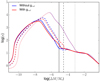 |
Fig. 5. Rosseland opacity profiles of the 1.4 M⊙ of grid 2 for XC = 0.6 (solid curves), XC = 0.4 (dashed curves), and XC = 0.2 (dotted curves). The blue and red curves represent respectively the models without and with grad. The solid dashed and dotted vertical lines represent the position of the bottom of the surface convection zone for the model without grad for the same value of XC as the opacity profiles (for clarity, they are not represented for the model with grad). |
As a result, the bottom of the surface convection zone is always deeper when grad is taken into account (see upper panels of Fig. 6) as was already shown by Turcotte et al. (1998a) for F-type stars. The more massive the star, the more important the deepening of the surface convection zone due to grad. Once again this effect is larger for lower metallicity stars. This maximum difference, which can be obtained from models with and without grad, reaches 120% for grid 1 and goes down to 65% and 5% for grids 2 and 3 for the more massive models of the three grids.
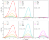 |
Fig. 6. Evolution of the difference of the mass of the surface convection zone (upper panels) and of the difference of the radius of the models (lower panels) with the frequency at maximum power νmax (see Sect. 4) for the three grids of models. Dashed lines are for the same models but without the effect of partial ionisation. |
WE note that the deepening of the convection zone is smaller in our models than in the Turcotte et al. (1998a) models. We presume that this could be due to the fact that the radiative acceleration for Ni, which significantly contributes to the opacity, is presently missing in our calculations. The new SVP tables that are in preparation (Alecian & LeBlanc, in prep., priv. comm.) should improve our models in the near future.
3.5. Variation of the stellar radius
We have seen in previous sections that the accumulation of metals modifies superficial abundances, opacity profiles, and size of the convection zone. Since the structure of the star is modified, so is the radius. Accurate knowledge of the radius is important in order to characterise exoplanets found by the transit method. If we compare the stellar radii computed without grad to those computed with grad (see lower panels of Fig. 6), models with grad always give larger radii. The maximum difference which can be obtained from models with and without grad never exceeds 2% and is at the level of requested uncertainties for the PLATO objectives. The increase in radius in our grad models is linked to a decrease in the mean density due to atomic diffusion including grad, the same effect (but smaller in magnitude) was found for the Sun by Turcotte et al. (1998b).
4. Seismic implications
Our study confirms that grad may have non-negligible effects on stars, especially on the iron surface abundance and on the size of the surface convection zone. Can these changes have detectable effects on the seismic properties of the star? We consider here only the global seismic indices, leaving a more comprehensive study of individual frequencies and frequency combinations for a forthcoming paper. The global asteroseismic indices are the frequency at maximum power, νmax, and the averaged large frequency separation, Δν0 (Chaplin et al. 2013). Scaling relations relating these seismic indices to stellar mass, radius, and effective temperature are expressed for solar-like oscillating main-sequence stars as (Kjeldsen & Beddinget al. 1995)
 (5)
(5)
 (6)
(6)
We showed that grad has an impact on Teff and on the radii of stars for a given mass (Sect. 3), so an effect should be visible in the νmax and Δν values. In order to be detectable, the seismic signatures of the grad must be larger than the uncertainties arising from the observations. The Kepler Legacy sample of solar-like oscillating stars includes stars in the mass range 0.8−1.6 M⊙ with [Fe/H] in the range [−1,+0.5] dex (Silva Aguirre et al. 2017). For most of these stars, Lund et al. (2017) obtained uncertainties for νmax and Δν in the approximate range 6–50 μHz and 0.05–0.2 μHz, respectively, depending on the apparent magnitude (in the range 6–11 mag) and the observing time (between 12 months and more than four years). The PLATO mission aims to measure individual frequencies of a reference star (1 M⊙,1 R⊙, 6000 K) with uncertainties no larger than 0.2 μHz at magnitude 10 (Rauer et al. 2014). The PLATO uncertainties for νmax and Δν are expected to lie in similar ranges to those of Kepler at a given magnitude, but PLATO will observe a larger number of bright stars and therefore with expected uncertainties on the lower side of the range. For the purpose of comparison, we considered two sets of uncertainties on νmax and Δν (see Table 3). The first set (A) is based on the uncertainties of the best Kepler Legacy data (Silva Aguirre et al. 2017; Lund et al. 2017) and the bulk of bright PLATO target stars. The second set (B) considers more conservative uncertainties. In the following we compare, for both sets, the effects of grad on νmax and Δν0.
Considered uncertainties on observed νmax and Δν0.
4.1. grad-induced change on νmax and Δν0
Figure 7 compares νmax and Δν0 for our selected sample of masses and metallicities at seven stages along the main-sequence. We find that the values of νmax and Δν0 are always lower for models including grad.
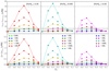 |
Fig. 7. Evolution with the central hydrogen content of the differences of frequency at maximum power, νmax, between models without and with grad for the three grids (upper panels). The same, but for the average large separation Δν0 (lower panels). Each colour corresponds to a given mass. The dashed lines represent the same models but without the effect of partial ionisation. The horizontal black dash-dotted lines indicate the adopted A uncertainty set, and the horizontal black dashed lines indicate the adopted B uncertainty set on νmax (upper panels) and Δν0 (lower panels). |
For νmax, the impact of grad never exceeds 15 μHz except for the most massive models. This is more than three times lower than uncertainty set B, but 2.5 times larger than uncertainty set A. We conclude that grad needs to be very efficient in order to produce a significant signature in the νmax value.
The effects on Δν0 are more important. The inclusion of grad leads to differences that reach 2.4 μHz (for the 1.4 M⊙ model at solar metallicity), which is much larger than any uncertainty derived from Kepler data or expected from PLATO data. Because Δν0 is directly related to the mean density of the star, differences in radius as small as 2% can still induce large differences in Δν0.
We can now define the mass limit ML as the stellar mass above which the change in Δν0 due to grad is larger than the uncertainties considered in sets A and B. For set A, the values of ML are 1.05, 1.25, and 1.4 M⊙, for grid 1, 2, and 3, respectively. In the case of set B, the values of ML are lower (0.9, 1.1, and 1.2 M⊙ for grid 1, 2, and 3, respectively). These values of ML are listed in Table 4, and serve as references. They correspond to the lowest masses below which grad can be neglected. For masses higher than these limits, the effect of grad will depend on the efficiency of other transport processes.
Mass above which grad has a non-negligible effect on seismic predictions.
4.2. grad-induced uncertainties on seismic ages
When modelling a star using seismic constraints, the impact of grad on νmax and Δν0 generates an uncertainty on the age of the star. An order of magnitude of the age uncertainty can be obtained for instance by comparing the ages of standard and grad models at fixed mass, metallicity, central hydrogen abundance, and Δν0. In such a configuration, we find that the age of the model with grad is always younger than that of the standard model in this study.
The maximum difference due to grad at metallicity [Fe/H]ini = 0.035 (grid 2) is obtained for the 1.4 M⊙ model at XC = 0.4 and Δν0 = 82.90 μHz. The ages of the corresponding standard and grad models are respectively 1.546 Gyr and 1.386 Gyr, that is they differ in age by about 9%. Similarly for the most massive models of grids 1 and 3, we obtain age differences of about 6% and 5%. The grad therefore contributes significantly to the age error budget for the most massive main-sequence stars showing solar-like oscillations.
4.3. Acoustic depths of the base of the convection zone
In Sect. 3.4 we showed that the depth of the surface convection zone increases when grad is included. The question then is whether the grad-induced change of the size of the CZ is significant. Solar-like oscillations enable the measurement of the acoustic depth of the base of the convection zone which is defined as
 (7)
(7)
where rCZ is the radius of the bottom of the surface CZ, cs the sound speed, and R∗ the radius of the star (Mazumdar & Antia 2001, and references therein). We therefore computed the acoustic depths, τCZ,obs, for our models and compared the resulting grad-induced differences ΔτCZ,RA to the observational uncertainties of seismically measured τCZ,RA. From our models, we find that the maximum grad-induced differences for the convective sizes roughly correspond to ΔτCZ,RA ∼ 300 s for the 1.4 M⊙ model of grid 2 and to 340 s for the 1.2 M⊙ model of grid 1 at fixed XC. This difference goes down to 160 s for the first case when comparing models with the same radius. Seismically measured τCZ,obs were obtained by Verma et al. (2017) for stars from the Kepler Legacy sample. These authors found typical uncertainties on τCZ,obs of the order of 150 s for stars with masses of about 1.4 M⊙ and of the order of 75 s for stars with masses of about 1.2 M⊙. Thus, we can conclude that grad must be taken into account in the models in order to determine the properties at the base of the convection zone for the most massive stars in the range of interest showing solar-like oscillations.
5. Impact of grad on [Fe/H] and on the stellar parameter determinations
With CoRoT and Kepler high-quality seismic data it is possible to determine very precise stellar parameters such as masses, radii, and ages for solar-like oscillating dwarfs (Lebreton & Goupil 2014; Silva Aguirre et al. 2017; Reese et al. 2016). In that framework, one significant impact of the grad on the stellar parameter determination is its effect on the relation between the iron content and the metallicity.
Today, a stellar parameter determination is usually achieved by means of an optimisation process. This method looks for the stellar model that best fits the observed oscillation frequencies and/or frequency combinations and additional spectroscopic constraints such as the effective temperature and/or log g. The stellar model computations involved in the best-fit search require the knowledge of the initial metallicity Zini. However, the available spectroscopic constraint used for the best-fit search is the surface iron abundance of the star [Fe/H] determined from observations. Assuming a chemical mixture scaling, we derive the current surface metallicity Zs. However, this quantity can significantly differ from the initial metallicity Zini of the star due to internal transport processes occurring over time. In particular, grad can lead to an accumulation of iron at the surface. This means that we must expect a lower initial iron abundance than the observed value. When only gravitational settling is taken into account, the effect is the opposite.
In addition to these difficulties, we emphasise that atomic diffusion, especially grad, acts differently on the chemical elements. Then when iron accumulates at the surface of the star, it is no longer possible to approximate the surface metallicity Zs using the determination of [Fe/H] by spectroscopy. Figure 8 compares the values of [Fe/H] considering the surface abundances of iron and hydrogen following Eq. (4), and considering that [Fe/H] = [M/H], i.e. [Fe/H] is assimilated to the surface metal to hydrogen abundance ratio.
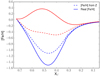 |
Fig. 8. Comparison between [Fe/H] computed with the real surface abundance of iron and hydrogen (solid lines) and computed from the metallicity value (dashed lines) for 1.4 M⊙ models with (red curves) and without (blue curves) grad. |
When considering only gravitational settling (blue curves), the difference between the two computation methods gives similar evolutions of the profiles for 1.4 M⊙. Nevertheless there are differences up to 0.4 dex that are much larger than current observational uncertainties. As the elements are diffusing toward the centre but at different velocities, the scaling of the iron abundance with Z is not possible even in that case. The difference reaches 0.7 dex for the models including grad (red curves) and the evolution is completely different as the iron is accumulated at the surface. In this case iron does not follow the behaviour of other heavy elements (namely CNO) for which gravitational settling dominates the diffusion. It is clear in this example that the [Fe/H] value needs to be computed with the actual value of iron and hydrogen abundances. The differences between the two methods used to compute [Fe/H] are smaller for lower mass stars and/or when other transport processes are taken into account since atomic diffusion is less effective. This issue needs to be investigated, especially in the framework of optimisation methods as evolution codes used to compute stellar models rarely follow the evolution of the iron abundance.
6. Discussion
6.1. Impact of partial ionisation
In all the comparisons we have made on the structural and seismic properties, we observe that neglecting partial ionisation strongly underestimates the impact of atomic diffusion, especially for the most massive stars of our grids. As shown in Figs. 4, 6, and 7, the impact is roughly doubled when partial ionisation is taken into account. This occurs because iron dominates the structure modifications, and because it is among the elements we consider, the one for which neglecting partial ionisation in estimating the mean electric charge induces the largest errors (it has the highest atomic number). It is clear from this study that partial ionisation must be taken into account in modelling main-sequence stars.
6.2. Effect of the initial solar mixture
We demonstrated how the initial metallicity is an important parameter in evolution models including grad. To evaluate the impact of the adopted solar mixture, we compared models based on the solar mixture of AGSS09 to models based on Grevesse & Noels (1993; hereafter the GN93 mixture). We computed two 1.3 M⊙ models with the GN93 mixture, with and without grad, in order to perform the same comparisons as in Sect. 4.1. In these two models (Z/X)ini = 0.0276 and αCGM = 0.678 as inferred from a solar calibration.
The solar metallicity of the GN93 mixture is higher than the AGSS09 value. We showed in previous sections that grad decreases when the metallicity increases for a given mass. Therefore, the effect of grad is slightly smaller in models using the GN93 mixture, but is still non-negligible. With the GN93 mixture, the mass above which grad has non-negligible effects on seismic predictions is only ≈0.05 M⊙ higher than the mass limit obtained with the AGSS09 mixture (Table 4). The difference for other solar mixtures (Grevesse & Sauval 1998; Asplund et al. 2005) is expected to be smaller because the metallicity difference with AGSS09 is smaller.
6.3. Implications for the PLATO space mission
In Sect. 4.1, we determined that grad induces differences in νmax and Δν0 that can be larger than their observational uncertainties when the stellar mass lies above a lower mass limit ML, which depends on the metallicity (Table 4). These lower masses can be used to determine whether grad has to be taken into account to ensure a given accuracy on the inferred stellar parameters. We can estimate the number of stars of the PLATO core program which might be affected by grad. For this purpose we use a stellar population synthesis computed with the Besançon Galaxy model (Robin et al. 2003, 2014; Czekaj et al. 2014; A. Robin, priv. comm.). The simulation is representative of one PLATO observation field. The mass limits of Table 4 are indicated by yellow points (uncertainty set B) and orange points (uncertainty set A) in Fig. 9. The number of stars with masses higher than the mass limits ranges from 33% up to 59% (depending of the uncertainty criteria) of the PLATO core program star sample and reaches 58%–75% for the total field. This number is an upper limit, but nevertheless indicates that for a significant number of stars, grad may not be negligible and the determination of their parameters will require some care if the requested PLATO accuracy is required.
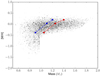 |
Fig. 9. Metallicity according to the mass of a population simulation of the PLATO (grey crosses) and Kepler (black crosses) core programme stars. The selected stars are from K7 to F5 with magnitudes in the range 4 < V < 11, effective temperature in the range 4030 < Teff < 6650 K, and luminosity classes between IV and V. The blue and red points correspond to the models listed in Table 4, which represent masses when grad needs to be taken into account. |
7. Conclusion
We improved the CESTAM code in order to compute models including the effects of radiative accelerations on the chemical element profiles and the resulting effects on opacities.
The goal was to characterise the sole transport effect of atomic diffusion including radiative accelerations; therefore, no macroscopic transport apart from convection was assumed. We computed two sets of models at three metallicities for masses ranging between 0.9 and 1.5 M⊙. One set includes the effect of grad and the other set does not.
The effects of radiative accelerations are higher at low metallicities and for the more massive stars considered here. The most obvious impact of radiative accelerations in stars is the modification of the surface abundances. For instance, this process is responsible for the surface abundances of chemically peculiar stars and we show here that it also has an impact for low-mass oscillating main-sequence solar-like stars. The most important abundance to follow is iron as it is one of the main contributors to opacity, while the [Fe/H] value is an important input for the stellar modelling. We showed that when radiative accelerations on iron are non-negligible it is not correct to calculate the [Fe/H] of a model simply considering a scaling of the metal content; the effect of radiative accelerations is selective, and even if iron accumulates at the surface the surface metallicity decreases as most of the other elements are depleted. This may have an important impact on the stellar parameter determination as [Fe/H] is an observational input. The difference in [Fe/H] between models with and without radiative accelerations reaches 1.7 dex for the more massive models of the grids.
We showed that the accumulation of elements in the surface convection zone (mainly iron) induces structure modifications. This is mainly due to the local increase of the opacity at the bottom of the surface convection zone as elements accumulate in regions where they are main contributors to the opacity. This local increase in the opacity leads to an increase in the size of the surface convection zone which can reach up to 120% in mass. This represents an increase larger than 160 s when considering the position of the bottom of the surface convection zone in acoustic radius. This is larger than the uncertainties obtained for some F-type stars of the Kepler Legacy sample and has to be further investigated. The modification of the radius of the star induced by the effects of radiative accelerations can reach 2%.
Using scaling relations we showed that the frequency at maximum power νmax of a model can be significantly affected by radiative accelerations for the more massive stars of our sample. Some models of our grid showed differences in the large frequency separation of pressure modes Δν0 that were larger than the observational uncertainty. For masses higher than 0.9, 1.1, and 1.2 M⊙ (considering uncertainties of the Kepler Legacy sample) respectively for [Fe/H]ini = −0.35, +0.035, and +0.25, radiative accelerations may have an impact on the age, mass, and radius determinations exceeding the precision requested by the PLATO main objectives. These masses are slightly higher when considering more conservative uncertainties. This has consequences on the parameters to be determined from Kepler, and future TESS and PLATO data. We estimated that radiative accelerations should be non-negligible for 33%–58% (depending on the considered uncertainties) of the core program stars of Kepler and PLATO.
It is important to note that the impact of radiative acceleration might be lowered when other processes are efficient in transporting material within stars, such as mixing induced by rotation, turbulence, or internal gravity waves to name a few. This is beyond of scope of this paper, but will be studied in a forthcoming work.
Acknowledgments
We acknowledge Annie Robin for providing us with the Besançon Galaxy models and Thierry Morel for fruitful discussions. This work was supported by CNES. We acknowledge financial support from the “Programme National de Physique Stellaire” (PNPS) of CNRS/INSU, France. This research was partially funded by the Natural Sciences and Engineering Research Council of Canada (NSERC). We thank Calcul Canada and Calcul Québec for computational resources. We acknowledge the referee for his careful reading and relevant suggestions which improved the paper.
References
- Adibekyan, V. Z., Sousa, S. G., Santos, N. C., et al. 2012, A&A, 545, A32 [NASA ADS] [CrossRef] [EDP Sciences] [Google Scholar]
- Alecian, G. 2018, ASP Conf. Ser., 515, 169 [NASA ADS] [Google Scholar]
- Alecian, G., & LeBlanc, F. 2000, MNRAS, 319, 677 [NASA ADS] [CrossRef] [Google Scholar]
- Alecian, G., & LeBlanc, F. 2002, MNRAS, 332, 891 [NASA ADS] [CrossRef] [Google Scholar]
- Alecian, G., & Stift, M. J. 2004, A&A, 416, 703 [NASA ADS] [CrossRef] [EDP Sciences] [Google Scholar]
- Alecian, G., & Stift, M. J. 2006, A&A, 454, 571 [NASA ADS] [CrossRef] [EDP Sciences] [Google Scholar]
- Alecian, G., Gebran, M., Auvergne, M., et al. 2009, A&A, 506, 69 [NASA ADS] [CrossRef] [EDP Sciences] [Google Scholar]
- Angulo, C. 1999, in AIP Conf. Ser., 495, 365 [NASA ADS] [CrossRef] [Google Scholar]
- Asplund, M., Grevesse, N., & Sauval, A. J. 2005, in Cosmic Abundances as Records of Stellar Evolution and Nucleosynthesis, eds. T. G. Barnes, & F. N. Bash, ASP Conf. Ser., 336, 25 [Google Scholar]
- Asplund, M., Grevesse, N., Sauval, A. J., & Scott, P. 2009, ARA&A, 47, 481 [NASA ADS] [CrossRef] [Google Scholar]
- Baglin, A., Michel, E., & Noels, A. 2013, in Progress in Physics of the Sun and Stars: A New Era in Helio- and Asteroseismology, eds. H. Shibahashi, & A. E. Lynas-Gray, ASP Conf. Ser., 479, 461 [Google Scholar]
- Bahcall, J. N., & Pinsonneault, M. H. 1992, Rev. Mod. Phys., 64, 885 [NASA ADS] [CrossRef] [Google Scholar]
- Bensby, T., Feltzing, S., & Oey, M. S. 2014, A&A, 562, A71 [NASA ADS] [CrossRef] [EDP Sciences] [Google Scholar]
- Brewer, J. M., Fischer, D. A., Valenti, J. A., & Piskunov, N. 2016, ApJS, 225, 32 [Google Scholar]
- Burgers, J. M. 1969, Flow Equations for Composite Gases (New York: Academic Press) [Google Scholar]
- Canuto, V. M., Goldman, I., & Mazzitelli, I. 1996, ApJ, 473, 550 [NASA ADS] [CrossRef] [Google Scholar]
- Chaplin, W. J., & Miglio, A. 2013, ARA&A, 51, 353 [NASA ADS] [CrossRef] [Google Scholar]
- Charpinet, S., Fontaine, G., Brassard, P., et al. 1997, ApJ, 483, L123 [NASA ADS] [CrossRef] [PubMed] [Google Scholar]
- Christensen-Dalsgaard, J. 2016, Lect. Notes Phys., in press [arXiv:1602.06838] [Google Scholar]
- Christensen-Dalsgaard, J., Proffitt, C. R., & Thompson, M. J. 1993, ApJ, 403, L75 [NASA ADS] [CrossRef] [Google Scholar]
- Claret, A., & Torres, G. 2016, A&A, 592, A15 [NASA ADS] [CrossRef] [EDP Sciences] [Google Scholar]
- Cunto, W., Mendoza, C., Ochsenbein, F., & Zeippen, C. J. 1993, A&A, 275, L5 [NASA ADS] [Google Scholar]
- Czekaj, M. A., Robin, A. C., Figueras, F., Luri, X., & Haywood, M. 2014, A&A, 564, A102 [NASA ADS] [CrossRef] [EDP Sciences] [Google Scholar]
- Deal, M., Richard, O., & Vauclair, S. 2016, A&A, 589, A140 [NASA ADS] [CrossRef] [EDP Sciences] [Google Scholar]
- Deal, M., Escobar, M. E., Vauclair, S., et al. 2017, A&A, 601, A127 [NASA ADS] [CrossRef] [EDP Sciences] [Google Scholar]
- Deheuvels, S., Silva Aguirre, V., Cunha, M. S., et al. 2015, Eur. Phys. J. Web Conf., 101, 01013 [CrossRef] [Google Scholar]
- Deheuvels, S., Brandão, I., Silva Aguirre, V., et al. 2016, A&A, 589, A93 [NASA ADS] [CrossRef] [EDP Sciences] [Google Scholar]
- Dotter, A., Conroy, C., Cargile, P., & Asplund, M. 2017, ApJ, 840, 99 [NASA ADS] [CrossRef] [Google Scholar]
- Eddington, A. S. 1926, The Internal Constitution of the Stars (Cambridge: Cambridge University Press) [Google Scholar]
- Ferguson, J. W., Alexander, D. R., Allard, F., et al. 2005, ApJ, 623, 585 [NASA ADS] [CrossRef] [Google Scholar]
- Gilliland, R. L., Brown, T. M., Christensen-Dalsgaard, J., et al. 2010, PASP, 122, 131 [NASA ADS] [CrossRef] [Google Scholar]
- Grevesse, N., & Noels, A. 1993, in Origin and Evolution of the Elements, eds. N. Prantzos, E. Vangioni-Flam, & M. Casse, 15 [Google Scholar]
- Grevesse, N., & Sauval, A. J. 1998, Space Sci. Rev., 85, 161 [Google Scholar]
- Hu, H., Tout, C. A., Glebbeek, E., & Dupret, M.-A. 2011, MNRAS, 418, 195 [NASA ADS] [CrossRef] [Google Scholar]
- Hui-Bon-Hoa, A. 2008, Ap&SS, 316, 55 [NASA ADS] [CrossRef] [Google Scholar]
- Hui-Bon-Hoa, A. & Vauclair, S. 2018, A&A, 610, L15 [NASA ADS] [CrossRef] [EDP Sciences] [Google Scholar]
- Hui-Bon-Hoa, A., LeBlanc, F., & Hauschildt, P. H. 2000, ApJ, 535, L43 [NASA ADS] [CrossRef] [PubMed] [Google Scholar]
- Iglesias, C. A., & Rogers, F. J. 1996, ApJ, 464, 943 [NASA ADS] [CrossRef] [Google Scholar]
- Imbriani, G., Costantini, H., Formicola, A., et al. 2004, A&A, 420, 625 [NASA ADS] [CrossRef] [EDP Sciences] [Google Scholar]
- Kjeldsen, H., & Bedding, T. R. 1995, A&A, 293, 87 [NASA ADS] [Google Scholar]
- Korn, A. J., Grundahl, F., Richard, O., et al. 2007, ApJ, 671, 402 [NASA ADS] [CrossRef] [Google Scholar]
- LeBlanc, F., & Alecian, G. 2004, MNRAS, 352, 1329 [NASA ADS] [CrossRef] [Google Scholar]
- LeBlanc, F., Michaud, G., & Richer, J. 2000, ApJ, 538, 876 [NASA ADS] [CrossRef] [Google Scholar]
- LeBlanc, F., Monin, D., Hui-Bon-Hoa, A., & Hauschildt, P. H. 2009, A&A, 495, 937 [NASA ADS] [CrossRef] [EDP Sciences] [Google Scholar]
- Lebreton, Y., & Goupil, M. J. 2014, A&A, 569, A21 [NASA ADS] [CrossRef] [EDP Sciences] [Google Scholar]
- Lebreton, Y., Montalbán, J., Christensen-Dalsgaard, J., Roxburgh, I. W., & Weiss, A. 2008, Ap&SS, 316, 187 [NASA ADS] [CrossRef] [Google Scholar]
- Lund, M. N., Silva Aguirre, V., Davies, G. R., et al. 2017, ApJ, 835, 172 [CrossRef] [Google Scholar]
- Marques, J. P., Goupil, M. J., Lebreton, Y., et al. 2013, A&A, 549, A74 [NASA ADS] [CrossRef] [EDP Sciences] [Google Scholar]
- Mazumdar, A., & Antia, H. M. 2001, A&A, 368, L8 [NASA ADS] [CrossRef] [EDP Sciences] [Google Scholar]
- Michaud, G. 1970, ApJ, 160, 641 [Google Scholar]
- Michaud, G., & Proffitt, C. R. 1993, in IAU Colloq. 137: Inside the Stars, eds. W. W. Weiss, & A. Baglin, ASP Conf. Ser., 40, 246 [Google Scholar]
- Michaud, G., Richard, O., Richer, J., & VandenBerg, D. A. 2004, ApJ, 606, 452 [NASA ADS] [CrossRef] [EDP Sciences] [Google Scholar]
- Michaud, G., Richer, J., & Vick, M. 2011, A&A, 534, A18 [NASA ADS] [CrossRef] [EDP Sciences] [Google Scholar]
- Michaud, G., Alecian, G., & Richer, J. 2015, Atomic Diffusion in Stars (Springer International Publishing) [CrossRef] [Google Scholar]
- Montalbán, J., Théado, S., & Lebreton, Y. 2007, EAS Pub Ser., 26, 167 [CrossRef] [Google Scholar]
- Montmerle, T., & Michaud, G. 1976, ApJS, 31, 489 [NASA ADS] [CrossRef] [Google Scholar]
- Morel, P. 1997, A&AS, 124, 597 [NASA ADS] [CrossRef] [EDP Sciences] [MathSciNet] [PubMed] [Google Scholar]
- Morel, P., & Lebreton, Y. 2008, Ap&SS, 316, 61 [NASA ADS] [CrossRef] [MathSciNet] [Google Scholar]
- Paxton, B., Schwab, J., Bauer, E. B., et al. 2018, ApJS, 234, 34 [NASA ADS] [CrossRef] [EDP Sciences] [Google Scholar]
- Peimbert, M., Luridiana, V., & Peimbert, A. 2007, ApJ, 666, 636 [NASA ADS] [CrossRef] [Google Scholar]
- Rauer, H., Catala, C., Aerts, C., et al. 2014, Exp. Astron., 38, 249 [NASA ADS] [CrossRef] [Google Scholar]
- Reese, D. R., Chaplin, W. J., Davies, G. R., et al. 2016, A&A, 592, A14 [NASA ADS] [CrossRef] [EDP Sciences] [Google Scholar]
- Richard, O., Michaud, G., & Richer, J. 2001, ApJ, 558, 377 [NASA ADS] [CrossRef] [Google Scholar]
- Richard, O., Michaud, G., & Richer, J. 2002, ApJ, 580, 1100 [NASA ADS] [CrossRef] [Google Scholar]
- Robin, A. C., Reylé, C., Derrière, S., & Picaud, S. 2003, A&A, 409, 523 [NASA ADS] [CrossRef] [EDP Sciences] [Google Scholar]
- Robin, A. C., Reylé, C., Fliri, J., et al. 2014, A&A, 569, A13 [NASA ADS] [CrossRef] [EDP Sciences] [Google Scholar]
- Rogers, F. J., & Nayfonov, A. 2002, ApJ, 576, 1064 [Google Scholar]
- Seaton, M. J. 1997, MNRAS, 289, 700 [NASA ADS] [CrossRef] [Google Scholar]
- Seaton, M. J. 2005, MNRAS, 362, L1 [NASA ADS] [CrossRef] [Google Scholar]
- Seaton, M. J. 2007, MNRAS, 382, 245 [NASA ADS] [CrossRef] [Google Scholar]
- Seaton, M. J., Zeippen, C. J., Tully, J. A., et al. 1992, Rev. Mex. Astron. Astrofis., 23, 19 [NASA ADS] [EDP Sciences] [Google Scholar]
- Serenelli, A. M. 2010, Ap&SS, 328, 13 [NASA ADS] [CrossRef] [Google Scholar]
- Silva Aguirre, V., Lund, M. N., Antia, H. M., et al. 2017, ApJ, 835, 173 [NASA ADS] [CrossRef] [Google Scholar]
- Talon, S., Richard, O., & Michaud, G. 2006, ApJ, 645, 634 [NASA ADS] [CrossRef] [Google Scholar]
- Théado, S. 2012, in Progress in Solar/Stellar Physics with Helio- and Asteroseismology, eds. H. Shibahashi, M. Takata, & A. E. Lynas-Gray, ASP Conf. Ser., 462, 60 [NASA ADS] [Google Scholar]
- Théado, S., Vauclair, S., Alecian, G., & LeBlanc, F. 2009, ApJ, 704, 1262 [NASA ADS] [CrossRef] [Google Scholar]
- Théado, S., Alecian, G., LeBlanc, F., & Vauclair, S. 2012, A&A, 546, A100 [NASA ADS] [CrossRef] [EDP Sciences] [Google Scholar]
- Thoul, A., & Montalbán, J. 2007, EAS Pub. Ser., 26, 25 [CrossRef] [Google Scholar]
- Thoul, A. A., Bahcall, J. N., & Loeb, A. 1994, ApJ, 421, 828 [NASA ADS] [CrossRef] [Google Scholar]
- Turcotte, S., Richer, J., & Michaud, G. 1998a, ApJ, 504, 559 [NASA ADS] [CrossRef] [Google Scholar]
- Turcotte, S., Richer, J., Michaud, G., Iglesias, C. A., & Rogers, F. J. 1998b, ApJ, 504, 539 [NASA ADS] [CrossRef] [Google Scholar]
- Turcotte, S., Richer, J., Michaud, G., & Christensen-Dalsgaard, J. 2000, A&A, 360, 603 [NASA ADS] [Google Scholar]
- Verma, K., Raodeo, K., Antia, H. M., et al. 2017, ApJ, 837, 47 [NASA ADS] [CrossRef] [Google Scholar]
- Watson, W. D. 1971, A&A, 13, 263 [NASA ADS] [Google Scholar]
All Tables
All Figures
|
Fig. 1. Comparisons of abundance profiles for different elements according to log(ΔM/M*) (where ΔM is the mass between the considered layer and the surface) for a 1.4 M⊙ at Z = 0.025 and 400 Myr between a model computed with the Montreal/Montpellier code (blue dashed curves) and the CESTAM code (red solid curves). The solid vertical lines indicate the position of the bottom of the surface convection zone of the models. |
| In the text | |
|
Fig. 2. HR diagrams for initial [Fe/H]ini = −0.35 (top panel), [Fe/H]ini = 0.035 (middle panel), and [Fe/H]ini = +0.25 (lower panel). The dashed curves represent models without grad and the solid curves represent models including grad. Black symbols are stars from the Kepler Legacy sample (Lund et al. 2017; Silva Aguirre et al. 2017). |
| In the text | |
|
Fig. 3. Evolution of surface abundances ([X/H] calculated as in Eq. 4) with time for the eight elements in grid 2 at solar metallicity. The solid and dashed curves respectively represent models with and without grad. |
| In the text | |
|
Fig. 4. Evolution of the difference in [Fe/H] between models with and without grad for the three grids of models. XC is the central hydrogen mass fraction. The solid lines show the differences for models including the effect of partial ionisation, while the dashed lines show the differences when this process is not taken into account. |
| In the text | |
|
Fig. 5. Rosseland opacity profiles of the 1.4 M⊙ of grid 2 for XC = 0.6 (solid curves), XC = 0.4 (dashed curves), and XC = 0.2 (dotted curves). The blue and red curves represent respectively the models without and with grad. The solid dashed and dotted vertical lines represent the position of the bottom of the surface convection zone for the model without grad for the same value of XC as the opacity profiles (for clarity, they are not represented for the model with grad). |
| In the text | |
|
Fig. 6. Evolution of the difference of the mass of the surface convection zone (upper panels) and of the difference of the radius of the models (lower panels) with the frequency at maximum power νmax (see Sect. 4) for the three grids of models. Dashed lines are for the same models but without the effect of partial ionisation. |
| In the text | |
|
Fig. 7. Evolution with the central hydrogen content of the differences of frequency at maximum power, νmax, between models without and with grad for the three grids (upper panels). The same, but for the average large separation Δν0 (lower panels). Each colour corresponds to a given mass. The dashed lines represent the same models but without the effect of partial ionisation. The horizontal black dash-dotted lines indicate the adopted A uncertainty set, and the horizontal black dashed lines indicate the adopted B uncertainty set on νmax (upper panels) and Δν0 (lower panels). |
| In the text | |
|
Fig. 8. Comparison between [Fe/H] computed with the real surface abundance of iron and hydrogen (solid lines) and computed from the metallicity value (dashed lines) for 1.4 M⊙ models with (red curves) and without (blue curves) grad. |
| In the text | |
|
Fig. 9. Metallicity according to the mass of a population simulation of the PLATO (grey crosses) and Kepler (black crosses) core programme stars. The selected stars are from K7 to F5 with magnitudes in the range 4 < V < 11, effective temperature in the range 4030 < Teff < 6650 K, and luminosity classes between IV and V. The blue and red points correspond to the models listed in Table 4, which represent masses when grad needs to be taken into account. |
| In the text | |
Current usage metrics show cumulative count of Article Views (full-text article views including HTML views, PDF and ePub downloads, according to the available data) and Abstracts Views on Vision4Press platform.
Data correspond to usage on the plateform after 2015. The current usage metrics is available 48-96 hours after online publication and is updated daily on week days.
Initial download of the metrics may take a while.