| Issue |
A&A
Volume 618, October 2018
|
|
|---|---|---|
| Article Number | A151 | |
| Number of page(s) | 15 | |
| Section | Planets and planetary systems | |
| DOI | https://doi.org/10.1051/0004-6361/201832674 | |
| Published online | 22 October 2018 | |
Detection of scattered light from the hot dust in HD 172555★,★★
1
Institute for Particle Physics and Astrophysics, ETH Zurich,
Wolfgang-Pauli-Strasse 27,
8093
Zurich,
Switzerland
e-mail: englern@phys.ethz.ch
2
Max Planck Institute for Astronomy,
Königstuhl 17,
69117
Heidelberg,
Germany
Received:
19
January
2018
Accepted:
23
July
2018
Context. Debris disks or belts are important signposts for the presence of colliding planetesimals and, therefore, for ongoing planet formation and evolution processes in young planetary systems. Imaging of debris material at small separations from the star is very challenging but provides valuable insights into the spatial distribution of the so-called hot dust produced by solid bodies located in or near the habitable zone. We report the first detection of scattered light from the hot dust around the nearby (d = 28.33 pc) A star HD 172555.
Aims. We want to constrain the geometric structure of the detected debris disk using polarimetric differential imaging (PDI) with a spatial resolution of 25 mas and an inner working angle of about 0.1″.
Methods. We measured the polarized light of HD 172555, with SPHERE/ZIMPOL, in the very broadband (VBB) or RI filter (λc = 735 nm, Δλ = 290 nm) for the projected separations between 0.08″ (2.3 au) and 0.77″ (22 au). We constrained the disk parameters by fitting models for scattering of an optically thin dust disk taking the limited spatial resolution and coronagraphic attenuation of our data into account.
Results. The geometric structure of the disk in polarized light shows roughly the same orientation and outer extent as obtained from thermal emission at 18 μm. Our image indicates the presence of a strongly inclined (i ≈ 103.5°), roughly axisymmetric dust belt with an outer radius in the range between 0.3″ (8.5 au) and 0.4″ (11.3 au). An inner disk edge is not detected in the data. We derive a lower limit for the polarized flux contrast ratio for the disk of (Fpol)disk/F∗ > (6.2 ± 0.6) × 10−5 in the VBB filter. This ratio is small, only ~9%, when compared to the fractional infrared flux excess (≈ 7.2 × 10⁻⁴). The model simulations show that more polarized light could be produced by the dust located inside ≈2 au, which cannot be detected with the instrument configuration used.
Conclusions. Our data confirm previous infrared imaging and provide a higher resolution map of the system, which could be further improved with future observations.
Key words: planetary systems / scattering / stars: individual: HD 172555 / techniques: high angular resolution / techniques: polarimetric
The reduced images (FITS files) are available at the CDS via anonymous ftp to cdsarc.u-strasbg.fr (130.79.128.5) or via http://cdsweb.u-strasbg.fr/cgi-bin/qcat?J/A+A/618/A151
© ESO 2018
1 Introduction
Young stars are often surrounded by circumstellar dust debris disks or rings. These consist of solid bodies, such as planetesimals and comets, as well as large amounts of dust and small amounts of gas. Small dust grains with a broad size distribution are generated in steady collisions of solid bodies and perhaps by the evaporation of comets. Debris disks are usually recognized by infrared (IR) excess on top of the spectral energy distribution (SED) of the stellar photosphere because of the thermal emission of the heated dust grains (see, e.g., Wyatt 2008; Matthews et al. 2014, for a review). In scattered light, debris disks are usually very faint, i.e., >103 times fainter than the host star, and therefore they are difficult to image. To date, several dozen debris disks have been spatially resolved in various wavelength bands, from visible to millimeter, using various space and ground-based telescopes. These data provide important constraints on the debris disk morphologies (e.g., Moerchen et al. 2010; Schneider et al. 2014; Choquet et al. 2016; Olofsson et al. 2016; Bonnefoy et al. 2017).
In the absence of imaging data, the location of the bulk of dust in the system can be inferred from the grain temperature derived by SED modeling. Based on modeling results, most debris disks have been found to harbor warm dust, meaning that the temperature of small grains lies between 100 K and approximately 300 K (e.g., Moór et al. 2006; Trilling et al. 2008; Chen et al. 2011; Morales et al. 2011). Cold debris reside far away from the host star where their temperature does not exceed 100 K. The prominent analogs to warm and cold dust belts are the main asteroid belt at 2–3.5 au and the Kuiper belt between 30 and 48 au in the solar system (Wyatt 2008). Aside from this, several stars with hot disks have been found (Wyatt et al. 2007a; Fujiwara et al. 2009) based on the IR excess with an estimate temperature above 300 K. The stars that possess hot dust are very interesting targets because the submicrometer-sized grains at a small distance from a star could be a signpost for transient collision events. HD 172555 (HIP 92024, HR 7012) is one of the most studied objects among these special stellar systems (Cote 1987; Schütz et al. 2005; Chen et al. 2006; Wyatt et al. 2007b; Lisse et al. 2009; Quanz et al. 2011; Smith et al. 2012; Riviere-Marichalar et al. 2012; Johnson et al. 2012; Kiefer et al. 2014; Wilson et al. 2016; Grady et al. 2018).
HD 172555 is a V = 4.8m, A7V star (Høg et al. 2000; Gray et al. 2006) at a distance of 28.33± 0.19 pc (Gaia Collaboration 2016) and a member of the β Pictoris moving group. The deduced age for the group is 23 ± 3 Myr (Mamajek & Bell 2014). HD 172555 has a K5Ve low mass companion CD-64 1208, separated by more than 2000 au or 71.4″ (Torres et al. 2006). The Infrared Astronomical Satellite (IRAS) identified HD 172555 as a Vega-like star that has a large IR excess with an effective temperature of 290 K (Cote 1987). Mid-infrared (mid-IR) spectroscopy from the ground (Schütz et al. 2005) and 5.5–35 μm spectroscopy obtained with the Spitzer Infrared Spectrograph (IRS) show very pronounced SiO features (Chen et al. 2006, their Fig. 2d) indicating large amounts of submicron sized crystalline silicate grains with high temperatures (>300 K). Lisse et al. (2009) proposed, based on the spectral analysis of mineral features, that the IR-excess emission originates from a giant collision of large rocky planetesimals similar to the event that could have created the Earth–Moon system.
Until now, only one resolved image of the HD 172555 debris disk existed that was obtained in the Qa band (λc = 18.30 μm, Δ λ = 1.52 μm; hereafter Q band) with the Thermal-Region Camera Spectrograph (TReCS) at Gemini South telescope and described by Smith et al. (2012). They detected extended emission after subtraction of a standard star point spread function (PSF), which is consistent with an inclined disk with an orientation of the major axis of θ = 120°, an inclination of ≈ 75°, and a disk outer radius of 8 au. In Si-5 filter (λc = 11.66 μm, Δ λ = 1.13 μm; hereafter N band) data, the disk was not detected. Combining these results with the visibility functions measured with the MID-infrared Interferometric instrument (MIDI), Smith et al. (2012) concluded that the warm dust radiating at ~10 μm is located inside 8 au from the star or inside the detected 18 μm emission.
The proximity of the host star and strong excess in the mid-IR (LIR ∕L* = 7.2 × 10⁻⁴; Mittal et al. 2015) from hot dust, makes HD 172555 an excellent, yet challenging, object for the search of scattered light. In this paper, we report the first detection of scattered light from the hot debris disk around HD 172555 with polarimetric differential imaging (PDI).
We present the PDI data from 2015 taken with the Zurich IMaging POLarimeter (ZIMPOL; Schmid et al. 2018) at the Very Large Telescope (VLT) in Chile. The ZIMPOL instrument provides high-contrast imaging polarimetry, coronagraphy with a small inner working angle of ~0.1″, and high spatial resolution of ~25 mas. The next section presents the available data together with a brief description of the instrument. Section 3 describes the data reduction and Sect. 4 the obtained results. Section 5 includes analysis of the observed disk morphology and photometry. For the interpretation of the data, we calculated three-dimensional (3D) disk models for spatial distribution of dust to put constraints on the geometric parameters of the disk and to estimate the flux cancellation effects in the Stokes Q and U parameters. In Sect. 6, we compare our results with previous TReCS and MIDI observations (Smith et al. 2012). We also investigate the possible presence of a very compact dust scattering component that would not be detectable in our data. We conclude and summarize our findings in Sect. 7.
2 Observations
Observations of HD 172555 were taken in service or queue mode during six runs in 2015 as part of the open time program 095.C-192 using ZIMPOL, the visual subsystem of the SPHERE (Spectro-Polarimetric High-contrast Exoplanet REsearch) instrument. The SPHERE instrument was developed for high-contrast observations in the visual and near-IR spectral range and includes an extreme adaptive optics (AO) system and three focal plane instruments for differential imaging (Dohlen et al. 2006; Beuzit et al. 2008; Kasper et al. 2012; Fusco et al. 2014; Schmid et al. 2018).
The ZIMPOL polarimetry is based on a modulation–demodulation technique and our observations of HD 172555 in the very broadband (VBB) filter were carried out in the fast modulation mode using field stabilization, which is also known as the P2 derotator mode. The ZIMPOL modulation technique measures the opposite polarization states of incoming light quasi-simultaneously and with the same pixels such that differential aberrations between I⊥ and I∥ are minimized. Fast modulation means a polarimetric cycle frequency of 967.5 Hz, which is obtained with a ferro-electric liquid crystal (FLC) and a polarization beam splitter in front of the demodulating CCD detector. The high detector gain of 10.5 e−/ADU allows broadband observations with high photon rates without pixel saturation and ensures high sensitivity at small angular separations at the expense of a relative high readout noise. The ZIMPOL VBB or RI filter used (λc = 735 nm, Δ λ = 290 nm) covers the R band and I band. Polarimetric data were taken in coronagraphic mode using the Lyot coronagraph V_CLC_MT_WF with a diameter of 155 mas. The mask is semi-transparent such that the central star is visible as faint PSF in the middle of attenuation region if the stellar PSF is of good quality (good AO corrections) and well centered on the mask. Short flux calibrations (the star was offset from the coronagraphic mask) with detector integration time (DIT) of 1.2 s and total exposure time of 14.4 s were also taken in each run using the neutral density filter ND2 with a transmission of about 0.87% for the VBB filter to avoid heavy saturation of the PSF peak.
The ZIMPOL instrument is equipped with two detectors/cameras, cam1 and cam2, which both have essentially the same field of view of 3.6″ ×3.6″. The format of the processed frame is 1024 × 1024 pixels, where one pixel corresponds to 3.6 × 3.6 mas on sky.The spatial resolution of our data provided by the AO system is about 25 mas.
The HD172555 data were taken at three different sky orientations on the CCD detectors with position angle (PA) offsets of 0°, 60°, and 120° with respect to sky north. For each field orientation, eight polarimetric QU cycles were recorded consisting each of four consecutive exposures of the Stokes linear polarization parameters + Q, − Q, + U, and − U using half-wave plate (HWP) offset angles of 0°, 45°, 22.5°, and 67.5°, respectively.For each exposure, eight frames with DIT of 10 s were taken and this yields a total integration of 10 s × 8 frames × 4 exposures × 8 cycles or ~42.7 min. Because of a timing error in the control law (see Maire et al. 2016) of the derotator during the first three runs performed in June 2015, the program was re-executed in August and September 2015. However, it turned out that this timing error was so small that itdoes not significantly affect the imaging of an extended source at small separation. Therefore, none of the six disk observationsfor HD 172555 are degraded by this effect. All our deep polarimetric observations of HD 172555 are listed in Table 1 together with the observing conditions, which have an important impact on the data quality.
Log of observations with the atmospheric conditions for each run.
3 Data reduction
The data were reduced with the SPHERE/ZIMPOL data reduction pipeline developed at ETH Zurich. We applied very similar procedures as in Engler et al. (2017) using flux normalization before polarimetric combination of the data.
For high-contrast polarimetry at small separations from the star, an accurate centering and the correction of the ZIMPOL polarimetric beam-shift are important (Schmid et al. 2018). The stellar position behind the mask should be determined with a precision higher than 0.3 pixels, otherwise the final image shows strong offset residuals disturbing the detection of a faint polarimetric signal. For the fine centering, we fitted a 2D Gaussian function using a central subimage with a radius of eight pixels containing the stellar light spot transmitted through a semitransparent coronagraphic focal plane mask.
The output of the data reduction pipeline consists of images of the intensity or Stokes I and the Stokes Q and U fluxes, where Q = I0 − I90 is positive for a linear polarization in N–S direction and U = I45 − I135 is positive for a polarization in NE–SW direction. For the data analysis, we transformed the Q and U images into a tangential or azimuthal polarization images Qφ and Uφ, locally defined with respect to the central light source. This transformation is useful for an optically thin circumstellar scattering region because the polarization signal is mainly in the Qφ component, while Uφ should be zero (e.g., Schmid et al. 2006; see also Appendix A).
During the data reduction, it turned out that an accurate centering of our HD 172555 images is difficult and not possible for a substantial portion of our data because several runs suffered from mediocre atmospheric conditions with a seeing > 1″ and therefore strongly reduced AO performance. Because of this problem only data from the best night 177 (2015-06-26; see Table 1) with an average seeing of 0.78″ and most data from the second best night 249 (2015-09-06) with seeing of 0.93″ could be used for our high-contrast polarimetry. Figure B.1 shows the Stokes I, Q, and U images of these data sets in comparison with the reduced data from the other observing runs that were affected by poor observing conditions.
To have a higher S/N per resolution element, images were 8 × 8 (Fig. 1) binned for the data analysis and modeling. In Fig. 2 we used a smaller binning (6 × 6) to preserve thespatial information and to have a more detailed picture of the disk.
4 Features in the reduced data
The top row of Fig. 1 shows the main results of our data reduction, i.e., the mean intensity or Stokes I, Stokes Qφ, and Uφ images using all eight cycles of the best night. The second row shows the same for six out of eight cycles from the second best night. The bottom row is the mean of these data.
The quality of the data can be easily recognized in the coronagraphic intensity images. These images show, for the best night (top), a much weaker halo and a weaker speckle ring at a separation of about r ≈ 0.35″ than for the second best night (middle). For all other nights, the disturbing light halo and speckles from the central star are even stronger (see Fig. B.1). Also clearly visible in Fig. 1 is the rotated speckle pattern in the top I image, which was taken with a field orientation of 120°, with respect to the middle I image taken without field orientation offset or 0°. In the latterimage, two strong quasi-static speckles from the AO system (indicated with white arrows) are located left and right from the central source on the speckle ring. The same speckles are rotated in the top image by 120° because of the applied field rotation.
The Qφ image from the best night in the top row shows a positive signal or tangential polarization for regions just ESE and WNW from the coronagraphic mask and some noisy features at the location of the two strong speckles. The corresponding Uφ image is also noisy but shows no predominant extended feature as seen in Qφ. The same ESE–WNW extension is also present in the Qφ image of thesecond best night, but now the disturbing strong speckles are adding noise in the E–W direction, particularly well visible in the Uφ image. Besides this, both Qφ and Uφ for the second best night show a quadrant pattern that is typical for a not perfectly corrected component from the telescope polarization. The following analysis of the disk morphology and modeling are based on the Qφ image in the top row obtained under the best observing conditions because these data are the least affected by noise.
The fact that we see the same kind of extended feature in the ESE-WNW orientation in both data sets (from the best and second best nights), while other features can clearly be associated with instrumental effects, strongly supports an interpretation that this is a real detection of the debris dust around HD 172555. This is further supported by the fact that the orientation and extent of the detected feature coincides at least roughly with the disk detection reported previously by Smith et al. (2012) based on imaging in the mid-IR.
In our image there is a prominent bright spot located below the coronagraphic mask. Most likely it is a spurious feature originating from image jitter and the temporal leakage of light of the central star from behind the coronagraphic mask. It is seen more particularly in 177 data set, which argues against this being a real feature.
A final remark on the data quality. Our data look noisy and are affected by not well corrected instrumental effects. However, we note that the signals in the Qφ and Uφ images are at a very low level of 0.001 of the signal in the intensity frame or the surface brightness in the Qφ image is on the order 10−5 of the expected peak flux of the central star for a separation of <0.3 arcsec. The detection of this faint target requires very high-contrast polarimetry at small angular separation. Not all instrumental effects are understood and can be calibrated at this level of sensitivity yet.
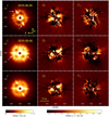 |
Fig. 1 Polarimetric differential imaging data of HD 172555 with the VBB filter (590–880 nm). The 8 × 8 binned images show polarized flux computed as Stokes I (left column), Qφ (middle column), and Uφ (right column) parameters. Top row: observation OBS177_0010-0042 (see Table 1 for the observational conditions) data averaged over 8 QU cycles. Middle row: observation OBS249_0028-0060 data averaged over 6 QU cycles. Bottom row: average of the data presented in the top and middle rows. The position of the star is denoted by a yellow asterisk. White arrows point out quasi-static speckles from the AO system. In all images north is up and east is to the left. The color bars show the counts per binned pixel. |
5 Analysis
5.1 Disk position angle and morphology
To determine the PA of the disk θdisk, we varied the position of the disk major axis in the range from θdisk = 105° to θdisk = 125° with a step of 0.5°. Each time the Qφ image was rotated by θdisk − 90° clockwise to place the disk major axis horizontally and then we determined the difference between the left side and the mirrored right side of the image. The minimum residual flux corresponding to the best match between disk sides is achieved at θdisk = 113.5° for the data set from 2015-06-26 (night 177) and at PA = 116.5° for the data set from 2015-09-06 (night 249).
We adopted the PA equal θdisk = 114° ± 3°. This PA should be corrected for the ZIMPOL True North offset of − 2°, which means the preprocessed image must be rotated by 2° clockwise. The final PA of the disk is, therefore, θdisk = 112° ± 3° north over east (NoE), where the indicated uncertainty includes associated systematic errors. For the following data analysis, the Qφ image was rotated by 24° clockwise, including the correction for the True Northoffset, to place the disk major axis horizontally. We introduced an x−y disk coordinate system with the star at the origin and the + x coordinate along the derived disk major axis in WNW direction and the y-coordinate perpendicular to this with the positive axis toward NNE (θ = 22°) as shown in Fig. 2b.
The observed Qφ flux image shows areas of enhanced surface brightness at the separations |x| ≃ 0.1−0.3″ but located about 0.04″ above the x-axis and this up-down asymmetry is reflected clearly in the surface brightness contours shown in Fig. 2b.
Figure 3 shows the profile for the polarized flux along the x-axis measured in bins of Δ x = 29 mas and integrated in the y-direction from y = −0.13″ to y = +0.16″. Our data show a higher flux closer to the star with a maximum flux inside r = 0.3″ and two small brightness peaks at |x|≈ 0.3″ (8.5 au) indicated with arrows “A” and “B” in Figs. 2b and 3.
Figure 3 also includes background profiles determined below and above the disk major axis by summing up the counts from y = −0.42″ to y = −0.13″ (light green dotted line) and from y = +0.16″ to y= +0.45″ (green solid line). The disk flux is at least twice as high as the background, except for a small region around x ≈ +0.23″ where the background is particularly high. The origin of the enhanced background below the disk midplane is unclear. The errors on flux per bin were calculated from the variance of the sum of pixel values in bins assuming a sample of normal random variables. The uncertainty of the pixel value is given by the standard deviation of the flux distribution (counts per pixel) computed in concentric annuli in the Qφ image (excluding the area containing the disk flux) to take into account the radial dependence of the data variance. As an additional noise estimator, we measured the background in the Uφ image (black solid line in Fig. 3) in the same areas where the polarized flux of the disk was measured in the Qφ image. The polarized scattered light from the disk is detected up to a radial distance of r ~ 0.8″. Beyond r = 0.3″, the polarized flux per x-bin is less than 8 ct s−1.
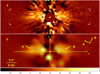 |
Fig. 2 Qφ image (panel a) and isophotal contours of polarized light intensity overlying the Qφ image (panelb). The original data (OBS177_0010-0042) were 6 × 6 binned to highlight the disk shape and to reduce the photon noise level. The position of the star is indicated by a yellow asterisk. White brackets in the top panel show the boundaries of two rectangular areas where the counts were summed up to retrieve the total polarized flux of the disk (see Sect. 5.3). Image (panel b) is smoothed via a Gaussian kernel with σkernel = 3 px. The isophotal contours show levels of the surface brightness with approximately 25, 40, and 50 counts per binned pixel (from the lowest to the highest contour). Arrows “A” and “B” mark the location of the increased surface brightness, which could indicate the radius of the planetesimal belt. The x-axis coincides with the disk axis at estimated PA θdisk = 112° (see Sect. 5). The color bar shows the surface brightness in counts per binned pixel. |
5.2 Modeling the observed disk flux
We modeled the spatial distribution of dust in HD 172555 disk with the 3D single scattering code presented in Engler et al. (2017). The disk geometry is described bya radius r0, where the radial distribution of the grain number density has a maximum, and by inner and outer radial power-law falloffs with exponents αin and αout, respectively.For the vertical distribution, we adopt the simpler Lorentzian profile instead of the exponential profile. The former profile has already been used for this purpose (e.g., Krist et al. 2005) and has an advantage that it is described with one parameter less. The Lorentzian profile is given by
![\[f_{\textrm{L}}(h)=a_{\textrm{L}}{\left[ 1 + \left(\frac{h}{H(r)}\right)^2\right]}^{-1} ,\]](/articles/aa/full_html/2018/10/aa32674-18/aa32674-18-eq2.png)
where h is the height above the disk midplane and aL is the peak number density of grains in the disk midplane. The scale height of the disk H(r) is defined as a half width at half maximum of the vertical profile at radial distance r and scales as in  .
.
The parameters of the model are the PA of the disk θdisk, the radius of the planetesimalbelt r0, inner αin and outer αout power law exponents, scale height H0, flare exponent β, inclination angle i, Henyey–Greenstein (HG) scattering asymmetry parameter gsca, and the scaling factor Ap. The scattering phase function for the polarized flux fp (θ, gsca) is the product fp (θ, gsca) = HG(θ, gsca) ⋅ pRay(θ) of the HG function and the Rayleigh scattering function (see Fig. 8 in Engler et al. 2017).
We assume that the debris disk is optically thin and neglect multiple scattering. The HG parameter has only positive values (0 ≤ gsca ≤ 1) assuming that the dust particles are predominately forward-scattering as inferred from imaging polarimetry of other highly inclined debris disks (e.g., Olofsson et al. 2016; Engler et al. 2017). This means that the brighter side of the disk is the near side and the inclination higher than 90° defines a disk with its near side toward north as in the case of the HD 172555 disk.
To simplify the model computation, we adopt the same grain properties everywhere in the disk. The averagescattering cross section per particle is a free parameter included in the scaling factor Ap.
The Qφ model image is calculated from the combination of the PSF convolved images of the Stokes parameters Q and U. The individual steps of the modeling procedure are described and illustrated in Appendix A.
To find parameters of the model that best fits the Qφ image (Fig. 4a), we took a twofold approach: first, we fitted the data with models drawn from a parameter grid and second we used the Markov chain Monte Carlo (MCMC) technique.
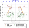 |
Fig. 3 Radial polarized flux profile measured in the Qφ image per 0.029″(Δx) × 0.290″(Δy) bin (red solid line) compared with profiles of the best-fitting models and background. The background above (green solid line) and below (light green dotted line) the disk midplane and the background in the Uφ image (black solid line) are calculated as explained in Sect. 5. The upper limit is set for the polarized flux per bin for the disk regions beyond r = 0.53″. The arrows “A” and “B” point to the surface brightness peaks. |
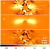 |
Fig. 4 Comparison of the grid model with the Qφ image. Panel a: Qφ image after 8 × 8 binning. Panel b: image of the best-fitting grid model convolved with the instrumental PSF. Panel c: residual image obtained after subtraction of the PSF-convolved grid model image (panel b) from the Qφ image (panel a). Color bar shows flux in counts per binned pixel. |
5.2.1 Grid of models
We define an extensive parameter grid of ~104 models and calculate a synthetic Qφ image for each model. The explored parameter space and steps of linear sampling are given in Table 2, Cols. 2 and 3. In this first modeling approach, the disk PA is set to θdisk = 112°, which is thePA value found in the previous section (Sect. 5.1). The flux scaling factor Ap is treated as a free parameter for each model and is obtained by minimizing the χ2 for the fit of the Qφ model image to the data. The reduced  metric is estimated as follows:
![\begin{equation*}\chi^2_{\nu} = \frac{1}{\nu}\sum_{i=1}^{N_{\textrm{data}}} \frac{\left[ F_{i,\, \textrm{data}}- A_{\textrm{p}}\cdot F_{i,\, \textrm{model}}(\vec{p})\right]^2 }{ \sigma_{i,\, \textrm{data}}^2} ,\end{equation*}](/articles/aa/full_html/2018/10/aa32674-18/aa32674-18-eq5.png) (1)
(1)
where Ndata is the number of pixels used to fit the data, Fi, data is the flux measured in pixel i with an uncertainty σi, data, and Fi, model(p) is the modeled flux of the same pixel. The degree of freedom of the fit is denoted by ν = Ndata − Npar, where Npar represents the number of model parameters  .
.
To be less affected by single pixel noise and to speed up this procedure, we reduce the number of pixels of the original Qφ image (Fig. 2a) by 8 × 8 binning and select a rectangular image fitting area with a length of 63 and width of 19 binned pixels (1.83″ × 0.55″; Fig. 4a) centered on the star. A round area with radius of 2.5 binned pixels covering the coronagraph and a few pixels around this region are excluded from the fitting procedure.
The minimum  is achieved for the model with parameters listed in Col. 4 of Table 2. Considering all the models that fit the observations well and have a
  we derive the parameter distribution and fit a Gaussian for each model parameter (see Fig. C.1). We adopt the mean valuesof the parameter distribution as the best-fitting model presented in Col. 5 of Table 2. The errors on the mean parameters are given by the 68% confidence interval derived for the respective distribution.
Disk model parameters.
5.2.2 MCMC modeling
We use the parameters of the best-fitting model from the parameter grid (Sect. 5.2.1) as a starting point for the MCMC run. To perform this analysis, we employed the Python module emcee by Foreman-Mackey et al. (2013), which implements affine invariant MCMC sampler suggested by Goodman & Weare (2010). The uniform priors are defined as specified in Col. 6 of Table 2. Contrary to the modeling with a grid of parameters (Sect. 5.2.1), the PA θdisk is allowed to vary.
For the run of the standard ensemble sampler, 1000 walkers are initialized to perform a random walk with 2000 steps. The posterior distributions of the parameters shown in Fig. C.2 are obtained discarding the burn-in phase of 400 walker steps. The mean fraction of the accepted steps within the chain is 0.342 and the maximum autocorrelation time of parameter samples is 90 steps. This indicates a good convergence and stability of the chain by the end of the MCMC run (Foreman-Mackey et al. 2013).
A set of the most probable parameters, which are considered to be the parameters of the best-fitting MCMC model, is listed in Col. 7 of Table 2. These parameters are derived as the 50th percentile of the posterior distribution. Their lower and upper uncertainties are quoted based on the 16th and 84th percentiles of the samples, respectively. Figure C.2 demonstrates the degeneracy between some of the model parameters, for instance, between HG parameter gsca and inclination of the disk i or scale height H0.
5.2.3 Modeling results
The MCMC sampling result for the PA of the disk is essentially the same as the PA we found by subtracting one disk side from the other (Sect. 5.1). Regarding other parameters, the best-fitting grid model (Table 2, Col. 5) and the MCMC model (Table 2, Col. 7) are consistent with each other. They indicate a disk radius r0 between 10 and 12 au and a disk inclination of ≈103.5°. The scale height of the vertical profile H0 is 10–20 times smaller than the radius of the disk. According to the MCMC model, the outer density falloff is at least steeper than about αout = −7. It is not clear whether the disk is cleared inside r0 because the inner radial index αin is smaller than 3. Both models indicate a relatively high asymmetry parameter for scattering gsca ≈ 0.7. This result could be affected by a higher surface brightness, which we observe inside r = 0.2″. The flare index β is the only parameter that remains unconstrained in both modeling methods (grid and MCMC) showing a tendency to be 0.
Both models fit the Qφ image equally well according to the  metric: the grid model has a
  (ν = 1152) and the MCMC model has a
  (ν = 1151). The residual images of both models show no noticeable differences. Therefore, in Fig. 4, we show only the grid model in comparison to the Qφ image.
Also, the radial profiles for the polarized flux of both models, which are calculated in the same bins as in the Qφ image (Fig. 4a), are qualitatively very similar (cf. yellow solid and dotted lines in Fig. 3).
5.2.4 Modeling cancellation effect
The synthetic image of the best-fitting model (Fig. 4b) is important for a correction of the polarized flux due to the extended instrument PSF. One effect is the loss of polarization signal because parts of it are outside the flux integration aperture. The second and more important effect for compact sources is the polarization cancellation effect where the positive and negative Q flux features in the Stokes Q image, and similar for Stokes U, cancel each other substantially if their separation is not much larger than the PSF. As described in Schmid et al. (2006) and Avenhaus et al. (2014), this can easily cause a reduction of the measurable polarization flux by a factor of 2 or more, depending on the source geometry and PSF structure.
We determine the total polarized flux for our best-fit model before and after convolution with the instrument PSF and derive for the cancellation effect a factor of 0.61 for our observations of the HD 172555 debris disk. In addition, we find that only 82% of the polarized flux of the convolved images fall into the rectangular disk-flux measuring areas indicated by the white corners in Fig. 2a, while 4% of the flux is covered by the coronagraphic mask near the star and 14% of the polarized flux are distributed in a very low surface brightness halo further out.
5.3 Measured polarized flux contrast of the disk
To compare the polarized flux from the disk with the stellar flux, we first derive the expected count rates of the star in the coronagraphic image if there were no coronagraph hiding its PSF peak. This is obtained with the flux frames where the star is offset from the coronagraphic mask. We use two flux measurements from the nights when we obtained good results (177 and 249) and derive a mean count rate for the central star of (4.36 ± 0.08) × 105 counts per second (ct s−1) per ZIMPOL arm by summing up all counts registered within the aperture with a radius of 1.5″ (413 pixels). Then we correct with a factor of 1.007 for the coronagraph attenuation at a distance of 0.35″ from the stellar PSF peak and a factor of ~115 to account for the mean transmission of the neutral density filter ND2.0 in the VBB filter. We obtain an average count rate of (5.00 ± 0.14) × 107 ct s−1 per ZIMPOL arm for the expected flux of the central star for observation in the fast polarimetry mode with the pupil mask but without correction for the attenuation by the focal plane mask or ND2.0 filter.
For the disk, we derive the total polarized flux by summing up all the counts in two rectangular areas indicated with white brackets in Fig. 2a, from |x| = 0.08″ to 0.77″ along the major axis and from y = −0.13″ to 0.16″ perpendicular to it. The innermost regions with radial separations |x| < 0.08″ are largely hidden behind the coronagraphic mask, and therefore they are not included in this estimate. The total polarized flux in the VBB filter after the modulation–demodulation efficiency calibration amounts to 780 ± 150 (ESE side, left) and 760 ± 150 (WNW side, right) ct s−1 and per ZIMPOL arm. Therefore, the total net flux obtained by integrating over abovementioned areas is 1540 ± 300 ct s−1 per ZIMPOL arm.
This measured flux must still be corrected for the polarimetric cancellation effects to get a value for the intrinsic polarized flux. Because of the limited spatial resolution of our data, the polarization in the positive and negative Q regions is reduced since signals with opposite signs overlap and cancel each other. We quantified this effect and calculated correction factors using our best-fit model (see description in the last paragraph of Sect. 5.2).
Taking into account the PDI efficiency, which causes the reduction of disk polarized flux by a factor of ~1.7 and correction factor for the aperture size (see Sect. 5.2), the total polarized flux of the disk is at least twice as large as the total net flux and is equal to 3100 ± 600 ct s−1 per ZIMPOL arm. This flux corresponds to the intrinsic modeled polarized flux compatible with our observation.With this value, the lower limit for the ratio of the disk total polarized flux to the stellar flux is  (cf. with the ratio
  obtained for the net flux
  ct s−1).
5.4 Polarimetric flux
To check our photometry, we compare the measured stellar flux with the stellar magnitudes from the literature. The stellar count rate of (4.36 ± 0.08) × 105 ct s−1 per ZIMPOL arm before correction for the transmission of the neutral density filter can be converted to the photometric magnitude m(VBB) (Schmid et al. 2017) as follows:
![\[m(\mathrm{VBB}) = -2.5 \log (\mathrm{ct\,s^{-1}})-\mathrm{am}\cdot k_1(\mathrm{VBB})-m_{\mathrm{mode}}+ \mathit{z}p_{\mathrm{ima}}(\mathrm{VBB}) ,\]](/articles/aa/full_html/2018/10/aa32674-18/aa32674-18-eq15.png)
where am = 1.3 is the airmass, k1 (VBB) = 0.086m is the filter coefficient for the atmospheric extinction, zpima(VBB) = 24.61m is the photometric zero point for the VBB filter, and mmode = 5.64m is an offset to the zero point, which accounts for the instrument configuration, pupil stop (STOP1_2), neutral density filter ND2.0, and the fast polarimetry detector mode. For HD 172555, we derive a magnitude m(VBB) = 4.68m ± 0.03m (indicated with a black asterisk in Fig. 5). This value is in good agreement with the Johnson photometric magnitude in R band m(R) = 4.887m ± 0.023m and I band m(I) = 4.581m ± 0.025m (Johnson et al. 1966).
For the estimated above ratio of the disk total polarized flux to stellar flux  , disk magnitude in the VBB filter is mpdisk(VBB) = 15.20m± 0.37m (indicated with a blue asterisk in Fig. 5).
At radial separation of r ≈ 0.3″ indicated with arrows “A” and “B” in Figs. 2b and 3, the peak surface brightness is ~15 ct s−1 per binned pixel (0.029″ × 0.029″) and corresponds to the SBpeak(VBB) = 13.3m ± 0.3m arcsec−2 or surface brightness contrast for the polarized flux of SBpeak(VBB) − mstar(VBB) = 8.62 mag arcsec−2.
6 Discussion
6.1 Comparison with thermal light detection and interferometry
The disk geometry is consistent with the 18 μm image presented in Smith et al. (2012). They found two lobes of extended emission along PA = 110° with a separation of about 0.4″ from the star and a flux of 105 mJy. On top of this, they measured a roughly seven times stronger (732 mJy) unresolved dust component and a stellar flux of 202 mJy. In the N-band image the dust was not resolved by Smith et al. (2012), but their N-band MIDI interferometry resolved the dust fully, putting it at separations between > 0.035″ and <0.27″ (1 − 8 au). Therefore, we also expect that a lot of polarized light from the dust scattering contributes to the signal inside the inner working angle of the SPHERE/ZIMPOL observations at 0.12″, which cannot be measured.
The disk modeling of the infrared flux by Smith et al. (2012) yields a disk with radius r = 0.27″ and width dr = 1.2r, which is equivalent to the ring with constant surface brightness between 0.1″ and 0.4″, inclined at 75° to the line of sight and at PA = 120° for the disk major axis. We confirm these parameters with our observation and can provide more stringent parameters for the inclination and the disk orientation because of the higher spatial resolution of our data. Also the disk extension agrees, but it is notclear whether the scattered light emission and thermal emission should show the same radial flux distributions.
In Fig. 5, we compare the flux distribution λFλ from the stellar photosphere with the thermal emission of the disk and the polarized flux distribution measured in this work. Photometric data points of HD 172555 are listed in Table 3 and plotted as green diamonds in Fig. 5, which also includes a Spitzer/IRS spectrum1. The stellar spectral fluxdensity is approximated by a Planck function for the star temperature of 7800 K (Riviere-Marichalar et al. 2012). A black asterisk (labeled VBB) denotes the stellar magnitude measured in the VBB (this work). The near-IR aperture photometry of HD 172555 in the N and Q bands (green diamonds at 11.7 and 18.3 μm), performed by Smith et al. (2012) using TReCS imaging data, is indicated by capital letters N and Q. The thermal flux from the disk is shown as a blackbody emission with the temperature of 329 K found by Riviere-Marichalar et al. (2012; orange solid line). The net polarized flux measured in the Qφ image (Sect. 5.3) is indicated by a light blue asterisk (labeled with Ipol = Qφ), and the polarized flux corrected for the polarimetric cancellation effects and aperture size is indicated by a blue asterisk in this figure. The blue dotted line shows an approximate curve for the SED of the polarized light obtained by scaling down the SED of the star. Using our best-fitting grid model, we roughly estimated the scattered flux from the disk (averaged over full solid angle) in the VBB filter. This conversion neglects the contribution from the diffracted light and assumes that the maximum polarization fraction of the phase function for the polarized flux is pmax = 0.3. This value is denoted with a yellow asterisk and labeled ⟨Isca⟩. We used this magnitude as a proxy for the scattered flux of the disk to compare it with the maximum thermal flux of the disk at λ = 10 μm and thus to estimate a kind of the disk albedo. We obtain ⟨ Isca⟩ (pmax = 0.3)/λFλ (λ = 10 μm) = 0.54, which should be considered as a very rough estimate for this ratio. The lower and upper limits on the scattered flux Isca, shown in Fig. 5, are obtained assuming maximum polarization fraction pmax = 0.1 (for the upper limit) and pmax = 0.7 (for the lower limit).
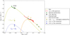 |
Fig. 5 Photometry of the star and disk together with the blackbody SED fits. |
Photometry of HD 172555.
6.2 Hidden source of thermal emission
According to the mid-IR observations of Smith et al. (2012), most of the dust is located inside 8 au, down to 1 au. Therefore, we investigate with model calculations whether a strong but compact source of scattered light could be present, which is notdetectable in our data because of the limited resolution and inner working angle limit of the used coronagraph.
The occulting spot in our coronagraphic data has a radius r ~ 0.08″ (2.27 au). We model a small disk with a radius of 2 au (0.07″) with exactly the same geometric morphology as the best-fit grid model derived in Sect 5.2, but just smaller by a factor of 5. This small disk is shown als Qφ image in Fig. 6a, together with the convolved Qφ image with the size of the coronagraphic mask indicated in Fig. 6b. First, we notice a large difference between Qφ intrinsic polarized flux and the convolved polarized flux of a factor of 2.5 because of the very strong polarimetric cancellation for such a compact disk. Then, there is another factor 2.67 between the total convolved polarized flux from the disk and the convolved polarized flux that falls into the rectangular measuring areas of our observations shown in Fig. 2a because a major region of the polarization signal is hidden by the coronagraphic mask. Thus, only about 15 % of the polarized flux produced by an inner compact disk would contribute to our measurement. We measure a net flux of 1540 ct s−1 in the measuring area of our observation and estimate that it is not possible to recognize an inner disk in our data, which contributes less than 150 ct s−1 to our measurement. Thus, an unseen compact disk with the geometry as described above and an intrinsic polarized flux of 6.675 × 150 ct s−1 could be present without being in conflict with our observations and even more scattered light could be hidden for a more compact inner disk.
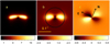 |
Fig. 6 Model of the small debris disk that could be hidden behind the coronagraphic mask. The model parameterscorrespond to those of the mean model (Table 2) except the radius of the belt and scale height of the dust vertical distribution, which are reduced by a factor of 5. Panel a: Qφ image of the debris disk model showing the polarized intensity before being convolved with the instrumental PSF. Panel b: Qφ image of the debris disk model showing the polarized intensity after convolution with the instrumental PSF. The black circle denotes the edge of the coronagraphic mask. Panel c: Uφ image of the model demonstrating nonzero Uφ signal appearing after convolution of the Stokes Q and U parameters with the instrumental PSF. The color bars show counts per pixel. |
6.3 Comparison between polarized flux and thermal emission
To characterize the scattering albedo of the dust, we compute the Λ parameter describing the ratio of the fractional polarized light flux to fractional infrared luminosity excess of the disk (Engler et al. 2017), i.e.,
where the ratio of total polarized flux of the disk to the stellar flux for HD 172555 is  (Sect. 5.3). Adopting the ratio of the disk infrared luminosity to stellar luminosity LIR ∕L* equal to 7.2 × 10⁻⁴ (Mittal et al. 2015), we obtain a lower limit for Λ ≥ 0.086. This value is slightly smaller than the Λ parameters we have estimated for the F star HIP 79977 and the M star AU Mic (ΛHIP 79977 = 0.11 and ΛAU Mic = 0.55) in Engler et al. (2017).
7 Summary
In this paper, we presented images of polarized scattered light from the debris disk around HD 172555 obtained in the VBB filter using differential polarimetry. We found that the observed polarized intensity is consistent with an axisymmetric dust distribution, which can be interpreted as a parent belt of planetesimals or disk with a radius in the range between 0.3″ (8.5 au) and 0.4″ (11.3 au). We analysed the disk structure and obtained the following results:
The PA for the disk major axis is θdisk = 112.3° ± 1.5° on the sky.
The diskemission is slightly shifted in NNE direction from the star indicating that the front side or forward-scattering part of the disk is on the NNE side. The observed dust distribution can be described with the HG asymmetry parameter g ≈ 0.7 and disk inclination ≈103.5°.
Data analysis and modeling results do not suggest the clearing of the inner disk regions (inside r = 0.3″).
The total disk magnitude in polarized flux in the VBB filter is mpdisk(VBB) = 15.20m ± 0.37m and the stellar flux is m(VBB) = 4.68m ± 0.03m. This gives a disk to star contrast
 of (6.2 ± 0.6) × 10−5. The measured peak surface brightness of the polarized light is SBpeak(VBB) = 13.3m ± 0.3m arcsec−2. This corresponds to a surface brightness contrast of SBpeak(VBB) − mstar(VBB) = 8.62 mag arcsec−2.
When compared with the fractional infrared luminosity of the disk using the Λ parameter, the fractional polarized light flux in the VBB filter makes up ~9%.
Our data demonstrate high sensitivity and ability of ZIMPOL to resolve the polarized light from the hot debris around a nearby A star as close as 0.1″ or ~3 au. It would be worth reobserving HD 172555 in the I band without the coronagraph. Additional observations of this target under excellent observing conditions, i.e., seeing ≤ 0.7, airmass ≤ 1.4, coherence time ≥3.5 ms, and wind speed >3 m s−1, to avoid the low wind effect (see SPHERE Manual) and with different offsets of the sky field on the detector would allow us to better distinguish between the instrumental features in the PSF and the real astrophysical signal. In the VBB filter, the speckle ring extends from 0.30″ to 0.45″ and overlaps the region of interest. In the I band, the speckle ring is further outside of ~0.40″ and the achievable contrast is higher under optimal observing conditions even if the amount of photons received in the I band is a factor of 0.6 lower than in the VBB. Moreover, noncoronagraphic data taken with I band are more suitable for the measurement of the beam shift between the two orthogonal polarization states and, hence, the correction of the beamshift effect (Schmid et al. 2018) is much easier. Such observation may also allow us to probe the innermost dust in the HD 172555 system.
Acknowledgements
We would like to thank the referee for many thoughtful comments that helped to improve this paper. This work is supported by the Swiss National Science Foundation through grant No. 200020 – 162630.
Appendix A Modeling the Qφ and Uφ images
Figure A.1 simulates the polarized flux measurement with the ZIMPOL instrument. In the first step, the distribution of the dust number density in the disk is generated using the parameters of the mean model. Then, synthetic images of debris disk in polarized light are calculated assuming only the single scattering of photons. An image of the polarized imtensity, or Qφ image (Fig. A.1a), is obtained considering angular dependence of polarization fraction on scattering angle θ such as that for Rayleigh scattering. Single scattering of photons produces linearly polarized light oriented perpendicular to the scattering plane, which corresponds to the azimuthal orientation of electric field in the 2D Qφ image. The Uφ image (Fig. A.1b) displays no signal because the Stokes Uφ parameter should show the polarization component in direction at 45° to the azimuthal direction. In this direction we do not expect to measure any signal if the assumption of single scattering is valid.
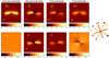 |
Fig. A.1 Model images of the polarized flux from HD 172555 debris disk. Images were generated using the parameters of mean model (Col. 5 in Table 2) and illustrate the individual steps of the modeling procedure (from left to the right panels) to obtain the final synthetic Qφ and Uφ images (panels g and h). For a detailed description of the presented images, see Appendix A. The diagram on the right side of the figure explains orientation of the axes used to measure the Stokes Q and U parameters as implemented in ZIMPOL instrument. The diagram shows also the orientation of north and east in each image. The north is rotated by 22° clockwise from the vertical line to have disk axis in horzontal position. Nonalignment of the disk axes with the Q and U measuring axes causes asymmetric flux distribution in Q and U images (panels c–f). |
In the following step, the Stokes Q and U images are calculated using the coordinate transformation:

where φ is the polar angle of each image point and is measured from NoE. This polar coordinate system corresponds to the measurement axes of the instrument shown on the right side of Fig. A.1. In ZIMPOL, the Stokes Q+ parameter is measured along north-south axis and the Stokes U+ parameter is measured along northeast-southwest axis.
The Q and U images (Fig. A.1c and d) are employed to create the images of individual polarization states I0, I45, I90, and I135. These images are firstly convolved with the PSF measured from the HD 172555 data and then are utilized to calculate new images of the Q and U parameters again but now in convolved state (Fig. A.1e and f). These two images imitate the output of the ZIMPOL data reduction pipeline. Usually they are used to compute the final Qφ and Uφ images of the disk applying reverse coordinate transformation as follows:

Examination of the final Qφ and Uφ images (Fig. A.1g and h) leads to two important conclusions. Comparison of the unconvolved and convolved Qφ images (Fig. A.1a and g) demonstrates the loss of a fraction of the polarized flux due to the convolution of the intensity of two orthogonal polarization states with the instrumental PSF (see also Sect. 5.2). As a result of blurring effect on the positive and negative signals in the Stokes Q and U due to the convolution with PSF, a nonzero signal is present in the final Uφ image (Fig. A.1h). For the mean model shown in Fig. A.1, the generated Uφ flux is of one order smaller thanthe Qφ flux that we measure in the Qφ image (Fig. A.1g). In general, this artificially created Uφ flux and the magnitude of the flux loss in the Qφ image depend on the geometry and extent of the polarized flux source and on the PSF structure. For the small compact sources, the generated Uφ flux and the PDI efficiency loss are the largest because the resolution of instrument is limited. Therefore, this effect should be estimated by means of modeling for each individual object and detector. To demonstrate this point, we calculate two additional models with the same parameters and the same aspect ratio of radius of the planetesimal belt to scale height as in the mean model but with different radii of the belts: one model with radius r = 2 au (0.07″) shown in Fig. 6and another model with the radius r = 30 au (1.05″). Our results show that the total polarized flux of the smaller debris disk is reduced by a factor of 0.4, whereas the extended disk suffers much less from the convolution effect and reducing factor is 0.73 for this disk.
Appendix B HD 172555 polarimetric data per observing run
Figure B.1 shows the reduced imaging data of HD 172555 from all six observing runs. The FITS files of the total intensity (Stokes I) and Stokes parameters Q and U of the data presented in rows two and four in this figure are also available in electronic form at the CDS.
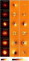 |
Fig. B.1 Reduced imaging data of HD 172555 from all six observing runs arranged from top to the bottom with the Stokes I (left column), Q (middle column) and U (right column) data. Each run was carried out with fixed sky orientation on the CCD detector with PA offset indicated in parenthesis. The highest quality observations are in rows two and four. To get north up and east to the left, each image should be rotated by the PA offset counterclockwise and the True North offset of the ZIMPOL should be taken into account. The yellow lines in the Q and U images show the position of disk major axis. |
Appendix C Probability distributions for fitted parameters
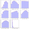 |
Fig. C.1 One-dimensional marginalized distributions of model parameters drawn from the sample of well-fitting models ( |

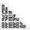 |
Fig. C.2 One- and two-dimensional posterior probability distributions of the fitted parameters. |
References
- Avenhaus, H., Quanz, S. P., Meyer, M. R., et al. 2014, ApJ, 790, 56 [NASA ADS] [CrossRef] [Google Scholar]
- Beuzit, J.-L., Feldt, M., Dohlen, K., et al. 2008, in Ground-based and Airborne Instrumentation for Astronomy II, Proc. SPIE, 7014, 701418 [NASA ADS] [Google Scholar]
- Bonnefoy, M., Milli, J., Ménard, F., et al. 2017, A&A, 597, L7 [NASA ADS] [CrossRef] [EDP Sciences] [Google Scholar]
- Chen, C. H., Sargent, B. A., Bohac, C., et al. 2006, ApJS, 166, 351 [NASA ADS] [CrossRef] [Google Scholar]
- Chen, C. H., Mamajek, E. E., Bitner, M. A., et al. 2011, ApJ, 738, 122 [NASA ADS] [CrossRef] [Google Scholar]
- Choquet, É., Perrin, M. D., Chen, C. H., et al. 2016, ApJ, 817, L2 [NASA ADS] [CrossRef] [Google Scholar]
- Cote, J. 1987, A&A, 181, 77 [NASA ADS] [Google Scholar]
- Dohlen, K., Beuzit, J.-L., Feldt, M., et al. 2006, Proc. SPIE, 6269, 62690Q [CrossRef] [Google Scholar]
- Engler, N., Schmid, H. M., Thalmann, C., et al. 2017, A&A, 607, A90 [NASA ADS] [CrossRef] [EDP Sciences] [Google Scholar]
- Foreman-Mackey, D., Hogg, D. W., Lang, D., & Goodman, J. 2013, PASP, 125, 306 [CrossRef] [Google Scholar]
- Fujiwara, H., Ishihara, D., Kataza, H., et al. 2009, in AKARI, a Light to Illuminate the Misty Universe, ed. T. Onaka, G. J. White, T. Nakagawa, & I. Yamamura, Astronomical Society of the Pacific Conference Series, 418, 109 [NASA ADS] [Google Scholar]
- Fusco, T., Sauvage, J.-F., Petit, C., et al. 2014, in Adaptive Optics Systems IV, Proc. SPIE, 9148, 91481U [NASA ADS] [CrossRef] [Google Scholar]
- Gaia Collaboration 2016, VizieR Online Data Catalog, 1337 [Google Scholar]
- Goodman, J., & Weare, J. 2010, Comm. App. Math. Comp. Sci., 5, 65 [Google Scholar]
- Grady, C. A., Brown, A., Welsh, B., et al. 2018, AJ, 155, 242 [NASA ADS] [CrossRef] [Google Scholar]
- Gray, R. O., Corbally, C. J., Garrison, R. F., et al. 2006, AJ, 132, 161 [NASA ADS] [CrossRef] [Google Scholar]
- Høg, E., Fabricius, C., Makarov, V. V., et al. 2000, A&A, 355, L27 [Google Scholar]
- Johnson, H. L., Mitchell, R. I., Iriarte, B., & Wisniewski, W. Z. 1966, Communications of the Lunar and Planetary Laboratory, 4, 99 [Google Scholar]
- Johnson, B. C., Lisse, C. M., Chen, C. H., et al. 2012, ApJ, 761, 45 [NASA ADS] [CrossRef] [Google Scholar]
- Kasper, M., Beuzit, J.-L., Feldt, M., et al. 2012, Messenger, 149, 17 [Google Scholar]
- Kiefer, F., Lecavelier des Etangs, A., Augereau, J.-C., et al. 2014, A&A, 561, L10 [NASA ADS] [CrossRef] [EDP Sciences] [Google Scholar]
- Krist, J. E., Ardila, D. R., Golimowski, D. A., et al. 2005, AJ, 129, 1008 [NASA ADS] [CrossRef] [Google Scholar]
- Lisse, C. M., Chen, C. H., Wyatt, M. C., et al. 2009, ApJ, 701, 2019 [NASA ADS] [CrossRef] [Google Scholar]
- Maire, A.-L., Langlois, M., Dohlen, K., et al. 2016, in Ground-based and Airborne Instrumentation for Astronomy VI, Proc. SPIE, 9908, 990834 [Google Scholar]
- Mamajek, E. E., & Bell, C. P. M. 2014, MNRAS, 445, 2169 [NASA ADS] [CrossRef] [Google Scholar]
- Matthews, B. C., Krivov, A. V., Wyatt, M. C., Bryden, G., & Eiroa, C. 2014, Protostars and Planets VI, 521 [Google Scholar]
- Mittal, T., Chen, C. H., Jang-Condell, H., et al. 2015, ApJ, 798, 87 [NASA ADS] [CrossRef] [Google Scholar]
- Moerchen, M. M., Telesco, C. M., & Packham, C. 2010, ApJ, 723, 1418 [NASA ADS] [CrossRef] [Google Scholar]
- Moór, A., Ábrahám, P., Derekas, A., et al. 2006, ApJ, 644, 525 [NASA ADS] [CrossRef] [Google Scholar]
- Morales, F. Y., Rieke, G. H., Werner, M. W., et al. 2011, ApJ, 730, L29 [NASA ADS] [CrossRef] [Google Scholar]
- Olofsson, J., Samland, M., Avenhaus, H., et al. 2016, A&A, 591, A108 [NASA ADS] [CrossRef] [EDP Sciences] [Google Scholar]
- Quanz, S. P., Kenworthy, M. A., Meyer, M. R., Girard, J. H. V., & Kasper, M. 2011, ApJ, 736, L32 [NASA ADS] [CrossRef] [Google Scholar]
- Riviere-Marichalar, P., Barrado, D., Augereau, J.-C., et al. 2012, A&A, 546, L8 [NASA ADS] [CrossRef] [EDP Sciences] [Google Scholar]
- Schmid, H. M., Joos, F., & Tschan, D. 2006, A&A, 452, 657 [NASA ADS] [CrossRef] [EDP Sciences] [Google Scholar]
- Schmid, H. M., Bazzon, A., Milli, J., et al. 2017, A&A, 602, A53 [NASA ADS] [CrossRef] [EDP Sciences] [Google Scholar]
- Schmid, H. M., Bazzon, A., Roelfsema, R., et al. 2018, A&A DOI: 10.1051/0004-6361/201833620 [Google Scholar]
- Schneider, G., Grady, C. A., Hines, D. C., et al. 2014, AJ, 148, 59 [NASA ADS] [CrossRef] [Google Scholar]
- Schütz, O., Meeus, G., & Sterzik, M. F. 2005, A&A, 431, 175 [NASA ADS] [CrossRef] [EDP Sciences] [Google Scholar]
- Smith, R., Wyatt, M. C., & Haniff, C. A. 2012, MNRAS, 422, 2560 [NASA ADS] [CrossRef] [Google Scholar]
- Torres, C. A. O., Quast, G. R., da Silva, L., et al. 2006, A&A, 460, 695 [NASA ADS] [CrossRef] [EDP Sciences] [Google Scholar]
- Trilling, D. E., Bryden, G., Beichman, C. A., et al. 2008, ApJ, 674, 1086 [NASA ADS] [CrossRef] [Google Scholar]
- Wilson, T. L., Nilsson, R., Chen, C. H., et al. 2016, ApJ, 826, 165 [NASA ADS] [CrossRef] [Google Scholar]
- Wyatt, M. C. 2008, ARA&A, 46, 339 [NASA ADS] [CrossRef] [Google Scholar]
- Wyatt, M. C., Smith, R., Greaves, J. S., et al. 2007a, ApJ, 658, 569 [NASA ADS] [CrossRef] [Google Scholar]
- Wyatt, M. C., Smith, R., Su, K. Y. L., et al. 2007b, ApJ, 663, 365 [NASA ADS] [CrossRef] [Google Scholar]
All Tables
All Figures
|
Fig. 1 Polarimetric differential imaging data of HD 172555 with the VBB filter (590–880 nm). The 8 × 8 binned images show polarized flux computed as Stokes I (left column), Qφ (middle column), and Uφ (right column) parameters. Top row: observation OBS177_0010-0042 (see Table 1 for the observational conditions) data averaged over 8 QU cycles. Middle row: observation OBS249_0028-0060 data averaged over 6 QU cycles. Bottom row: average of the data presented in the top and middle rows. The position of the star is denoted by a yellow asterisk. White arrows point out quasi-static speckles from the AO system. In all images north is up and east is to the left. The color bars show the counts per binned pixel. |
| In the text | |
|
Fig. 2 Qφ image (panel a) and isophotal contours of polarized light intensity overlying the Qφ image (panelb). The original data (OBS177_0010-0042) were 6 × 6 binned to highlight the disk shape and to reduce the photon noise level. The position of the star is indicated by a yellow asterisk. White brackets in the top panel show the boundaries of two rectangular areas where the counts were summed up to retrieve the total polarized flux of the disk (see Sect. 5.3). Image (panel b) is smoothed via a Gaussian kernel with σkernel = 3 px. The isophotal contours show levels of the surface brightness with approximately 25, 40, and 50 counts per binned pixel (from the lowest to the highest contour). Arrows “A” and “B” mark the location of the increased surface brightness, which could indicate the radius of the planetesimal belt. The x-axis coincides with the disk axis at estimated PA θdisk = 112° (see Sect. 5). The color bar shows the surface brightness in counts per binned pixel. |
| In the text | |
|
Fig. 3 Radial polarized flux profile measured in the Qφ image per 0.029″(Δx) × 0.290″(Δy) bin (red solid line) compared with profiles of the best-fitting models and background. The background above (green solid line) and below (light green dotted line) the disk midplane and the background in the Uφ image (black solid line) are calculated as explained in Sect. 5. The upper limit is set for the polarized flux per bin for the disk regions beyond r = 0.53″. The arrows “A” and “B” point to the surface brightness peaks. |
| In the text | |
|
Fig. 4 Comparison of the grid model with the Qφ image. Panel a: Qφ image after 8 × 8 binning. Panel b: image of the best-fitting grid model convolved with the instrumental PSF. Panel c: residual image obtained after subtraction of the PSF-convolved grid model image (panel b) from the Qφ image (panel a). Color bar shows flux in counts per binned pixel. |
| In the text | |
|
Fig. 5 Photometry of the star and disk together with the blackbody SED fits. |
| In the text | |
|
Fig. 6 Model of the small debris disk that could be hidden behind the coronagraphic mask. The model parameterscorrespond to those of the mean model (Table 2) except the radius of the belt and scale height of the dust vertical distribution, which are reduced by a factor of 5. Panel a: Qφ image of the debris disk model showing the polarized intensity before being convolved with the instrumental PSF. Panel b: Qφ image of the debris disk model showing the polarized intensity after convolution with the instrumental PSF. The black circle denotes the edge of the coronagraphic mask. Panel c: Uφ image of the model demonstrating nonzero Uφ signal appearing after convolution of the Stokes Q and U parameters with the instrumental PSF. The color bars show counts per pixel. |
| In the text | |
|
Fig. A.1 Model images of the polarized flux from HD 172555 debris disk. Images were generated using the parameters of mean model (Col. 5 in Table 2) and illustrate the individual steps of the modeling procedure (from left to the right panels) to obtain the final synthetic Qφ and Uφ images (panels g and h). For a detailed description of the presented images, see Appendix A. The diagram on the right side of the figure explains orientation of the axes used to measure the Stokes Q and U parameters as implemented in ZIMPOL instrument. The diagram shows also the orientation of north and east in each image. The north is rotated by 22° clockwise from the vertical line to have disk axis in horzontal position. Nonalignment of the disk axes with the Q and U measuring axes causes asymmetric flux distribution in Q and U images (panels c–f). |
| In the text | |
|
Fig. B.1 Reduced imaging data of HD 172555 from all six observing runs arranged from top to the bottom with the Stokes I (left column), Q (middle column) and U (right column) data. Each run was carried out with fixed sky orientation on the CCD detector with PA offset indicated in parenthesis. The highest quality observations are in rows two and four. To get north up and east to the left, each image should be rotated by the PA offset counterclockwise and the True North offset of the ZIMPOL should be taken into account. The yellow lines in the Q and U images show the position of disk major axis. |
| In the text | |
|
Fig. C.1 One-dimensional marginalized distributions of model parameters drawn from the sample of well-fitting models ( |
| In the text | |
|
Fig. C.2 One- and two-dimensional posterior probability distributions of the fitted parameters. |
| In the text | |
Current usage metrics show cumulative count of Article Views (full-text article views including HTML views, PDF and ePub downloads, according to the available data) and Abstracts Views on Vision4Press platform.
Data correspond to usage on the plateform after 2015. The current usage metrics is available 48-96 hours after online publication and is updated daily on week days.
Initial download of the metrics may take a while.