| Issue |
A&A
Volume 618, October 2018
|
|
|---|---|---|
| Article Number | A83 | |
| Number of page(s) | 25 | |
| Section | Extragalactic astronomy | |
| DOI | https://doi.org/10.1051/0004-6361/201732506 | |
| Published online | 16 October 2018 | |
Long-term optical, UV, and X-ray continuum variations in the changing-look AGN HE 1136-2304
1
Institut für Astrophysik, Universität Göttingen,
Friedrich-Hund Platz 1,
37077
Göttingen, Germany
e-mail: This email address is being protected from spambots. You need JavaScript enabled to view it.
2
Department of Earth and Space Sciences, Morehead State University,
Morehead,
KY
40351, USA
3
Astronomisches Institut, Ruhr-Universität Bochum, Universitätsstrasse 150,
44801
Bochum, Germany
4
Physics Department and the Haifa Research Center for Theoretical Physics and Astrophysics, University of Haifa,
Haifa
3498838, Israel
5
School of Physics & Astronomy and the Wise Observatory, The Raymond and Beverly Sackler Faculty of Exact Sciences Tel-Aviv University,
Tel-Aviv
69978, Israel
6
XMM-Newton Science Operations Centre, ESA, Villafranca del Casuntilo,
Apartado 78,
28691
Villanueva de la Cañada, Spain
Received:
20
December
2017
Accepted:
6
April
2018
Abstract
Aims. A strong outburst in the X-ray continuum and a change of its Seyfert spectral type was detected in HE 1136-2304 in 2014. The spectral type changed from nearly Seyfert 2 type (1.95) to Seyfert 1.5 type in comparison to previous observations taken ten to twenty years before. In a subsequent variability campaign we wanted to investigate whether this outburst was a single event or whether the variability pattern following the outburst was similar to those seen in other variable Seyfert galaxies.
Methods. In addition to a SALT spectral variability campaign, we carried out optical continuum, as well as X-ray and UV (Swift) monitoring studies from 2014 to 2017.
Results. HE 1136-2304 strongly varied on timescales of days to months from 2014 to 2017. No systematic trends were found in the variability behavior following the outburst in 2014. A general decrease in flux would have been expected for a tidal disruption event. This could not be confirmed. More likely the flux variations are connected to irregular fluctuations in the accretion rate. The strongest variability amplitudes have been found in the X-ray regime: HE 1136-2304 varied by a factor of eight during 2015. The amplitudes of the continuum variability (from the UV to the optical) systematically decreased with wavelength following a power law Fvar = a × λ−c with c = 0.84. There is a trend that the B-band continuum shows a delay of three light days with respect to the variable X-ray flux. The Seyfert type 1.5 did not change despite the strong continuum variations for the period between 2014 and 2017.
Key words: galaxies: active / galaxies: Seyfert / galaxies: nuclei / galaxies: individual: HE 1136-2304 / galaxies: photometry
© ESO 2018
1 Introduction
It is generally known that Seyfert 1 galaxies are variable in the optical and in X-rays on timescales of days to decades. Several active galactic nuclei (AGN) have shown variations in the X-ray continuum by a factor of more than 20 (e.g., Grupe et al. 2001, 2010). AGN that show extreme X-ray flux variations in combination with X-ray spectral variations, i.e., when a Compton-thick AGN becomes Compton-thin and vice versa, were designated as changing-look AGN (e.g., Guainazzi 2002). By analogy, optical changing-look AGN exhibit transitions from type 1 to type 2 and vice versa. In this case, the optical spectral classification can change due to a variation in the intrinsic nuclear power/accretion power, a variation in reddening, or a combination of the two. Typical transition timescales are months to years.
To date about a dozen Seyfert galaxies are known to have changed their optical spectral type, for example, NGC 3515 (Collin-Souffrin et al. 1973), NGC 4151 (Penston & Perez 1984), Fairall 9 (Kollatschny & Fricke 1985), NGC 2617 (Shappee et al. 2014), Mrk 590 (Denney et al. 2014) and references therein. Further recent findings are based on spectral variations detected by means of the Sloan Digital Sky Survey (e.g., Komossa et al. 2008; LaMassa et al. 2015; Runnoe et al. 2016; MacLeod et al. 2016). In most of these recent findings only a few optical spectra of the individual SDSS galaxies have been secured to prove their changing-look character.
HE 1136-2304 (α2000 = 11h38m51.1s, δ = − 23°21′36″) has been detected as a variable X-ray source by the XMM-Newton slew survey in 2014 (Parker et al. 2016). The 0.2–2 keV flux increased by a factor of about 30 in comparison to the ROSAT all-sky survey in 1990. However, no clear evidence of X-ray absorption variability has been seen. HE 1136-2304 changed its optical spectral classification from 1994 (Seyfert 2/1.95) to 2014 (Seyfert 1.5) and can be considered an optical changing-look AGN.
We decided to study the variability behavior of HE 1136-2304 subsequent to its X-ray outburst in 2014 in detail. We carried out optical photometric and spectroscopic variability follow-up studies in combination with Swift UV and X-ray photometric observations to investigate the variability behavior of this changing-look galaxy on timescales of weeks to years. The outburst in HE 1136-2304 could have been caused by a tidal disruption event, by a less drastic variation in the intrinsic nuclear power/accretion power, or by significant variation in the absorption. Although detailed and long-term optical variability studies exist for many AGN, for example NGC 5548 (Peterson et al. 2002; Pei et al. 2017), NGC 7603 (Kollatschny et al. 2000), and 3C 390.3 (Shapovalova et al. 2010), no detailed follow-up studies have been reported for the changing-look-type AGN mentioned above.
This is the first paper in a series. We will discuss the spectral variations seen in 2015 and the broad-line region structure in HE 1136-2304 in a second paper in detail.
Throughout this paper, we assume that H0 = 70 km s−1 Mpc−1 with a ΛCDM cosmology with ΩΛ = 0.73 and ΩM = 0.27. With a redshift of z = 0.0271 this results in a luminosity distance of DL = 118 Mpc using the Cosmology Calculator developed by Wright (2006).
Log of spectroscopic observations of HE1136 with SALT.
2 Observations and data reduction
2.1 Optical spectroscopy with the SALT telescope
We took a first optical spectrum of the Seyfert nucleus in HE 1136-2304 with the 10 m Southern African Large Telescope (SALT) nearly simultaneously with X-ray observations by XMM-Newton on 2014 July 07, just after the X-ray flaring (Parker et al. 2016). To study the subsequent variability behavior, we took additional optical spectra at 17 epochs with the SALT telescope between 2014 December 25 and 2015 July 13. To examine the long-term trend, four additional spectra were taken: three spectra in 2016 between January 12 and May 31 and one spectrum in 2017 on May 15. The log of our spectroscopic observations with SALT is given in Table 1. The Julian dates in all tables mark the beginning of the observations. We acquired 16 spectra between 2015 February and 2015 July with a mean interval of 9 days. The spacing of our observations was not regular. The shortest time interval between two subsequent observations was 4 days.
All spectroscopic observations were taken under identical instrumental conditions with the Robert Stobie Spectrograph attached to the SALT telescope using the PG0900 grating. The slit width was fixed to 2′′.0 projected onto the sky at an optimized position angle to minimize differential refraction. Furthermore, all observations were taken at the same air mass thanks to the particular design feature of the SALT. All spectra were taken with exposure times of 10 to 20 min (see Table 1). Typical seeing full width at half maximum (FWHM) values were 1 to 2 arcsec.
We covered the wavelength range from 4355 to 7230 Å at a spectral resolution of 6.5 Å. The observed wavelength range corresponds to a wavelength range from 4240 to 7040 Å in the rest frame of the galaxy. There are two gaps in the spectrum caused by the gaps between the three CCDs: one between the blue and the central CCD chip, and one between the central and red CCD chip covering the wavelength ranges 5206–5263 Å and 6254–6309 Å (5069–5124 Å and 6089–6142 Å in the rest frame). All spectra were wavelength corrected to the rest frame of the galaxy (z = 0.0271).
In addition to the galaxy spectra, we also observed necessary flat-field and Xe arc frames, as well as spectrophotometric standard stars for flux calibration (EG274, LTT3218, LTT7379). The spatial resolution per binned pixel was 0′′.2534 for our SALT spectra. We extracted eight columns from our object spectrum corresponding to 2′′.03. The reduction of the spectra (bias subtraction, cosmic ray correction, flat-field correction, 2D wavelength calibration, night sky subtraction, and flux calibration) was done in a homogeneous way with IRAF reduction packages (e.g., Kollatschny et al. 2001). We obtained typical S/N values of 40 in the continua of the galaxy spectra.
Great care was taken to ensure high-quality intensity and wavelength calibrations to keep the intrinsic measurement errors very low, as described in Kollatschny et al. (2001, 2003), Kollatschny & Zetzl (2010). Our AGN spectra and our calibration star spectra were not always taken under photometric conditions. Therefore, all spectra were calibrated to the same absolute [O III] λ5007 flux of 1.75 × 10⁻¹³ erg s−1 cm−2 (Reimers et al. 1996). The flux of the narrow emission line [O III] λ5007 is considered to be constant on timescales of many years. A relative flux accuracy on the order of 1% was achieved for most of our spectra.
2.2 Optical, UV, and X-ray observations with Swift
After the discovery of the X-ray flaring in June 2014 (Parker et al. 2016), we started monitoring HE 1136-2304 with Swift (Gehrels et al. 2004) in X-rays and the UV/optical. All Swift observing dates and exposure times are listed in Table A.4. In this paper, we focus on the Swift observations between 2014 June 06 and 2016 February 02. However, HE 1136-2304 had been observed previously by Swift during three epochs in 2010. For comparison purposes, we list these observations in all the tables relevant to Swift data (see Tables A.1, A.2, and A.4).
Most X-ray observations with the Swift X-ray Telescope (XRT; Burrows et al. 2005) were performed in photon counting mode (pc-mode; Hill et al. 2004). However, the four observations in 2014 August were performed in windowed timing mode. For the pc-mode data, source counts were collected in a circular region with a radius of 30 pixels (equivalent to 70″) and background counts in a nearby source-free circular region with a radius of 90 pixels (equal to 210″). The windowed timing source and background spectra were selected in boxes with a width of 40 pixels each. Spectra were extracted with the FTOOL XSELECT. An auxiliary response file (ARF) was created for each observation using xrtmkarf. We applied the Swift XRT response file swxpc0to12s6_20130101v014.rmf and swxwt0to2s6_20131212v015.rmf for the pc and WT data, respectively. Most spectra were rebinned to have at least 20 counts per bin using grppha. For some spectra the number of counts was too low to allow χ2 statistics. These data were fitted by Cash statistics (Cash 1979). The spectral analysis was performed in XSPEC (Arnaud 1996).
We fitted the X-ray spectra first with a simple power-law model with the absorption parameter fixed to the Galactic value. In addition, we fitted a power-law model with redshifted intrinsic absorption (zwa) to the data with the redshift fixed to the redshift of HE 1136-2304. For some spectra we found some evidence of a low intrinsic absorption on the order of 1 × 1021 cm−2; however, in most cases the absorption column density of the absorber was consistent with the Galactic value and the fits did not require any additional absorber. Finally, all spectra were fitted with a single power-law model with Galactic absorption (NH,gal = 3.3 × 1020 cm−2; Kalberla et al. 2005). As indicated in Table A.2, we also fitted the data with a redshifted intrinsic absorber model.
Count rates, hardness ratios, and the best fit values obtained are listed in Table A.2. The hardness ratio is defined as HR = counts(0.3–1.0 keV)/counts(1.0–10.0 keV). In order to determine a background corrected hardness ratio, we applied the program BEHR by Park et al. (2006).
During most observations, the Swift UV-Optical Telescope (UVOT; Roming et al. 2005) observed in all six photometricfilters UVW2 (1928 Å), UVM2 (2246 Å), UVW1 (2600 Å), u (3465Å), b (4392 Å), and v (5468 Å). Before analyzing the data, allsnapshots in one segment were combined with the UVOT tool uvotimsum. The flux densities and magnitudes in each filter were determined by the tool uvotsource using the count rate conversion and calibration, as described inPoole et al. (2008) and Breeveld et al. (2010). Source counts were extracted in a circle with a radius of 5″ and background counts in a nearby source-free region with a radius of 20″. The UVOT fluxes listed in Table A.1 are not corrected for Galactic reddening. The reddening value in the direction of HE 1136-2304 is EB-V = 0.03666, deduced from the Schlafly & Finkbeiner (2011) re-calibration of the Schlegel et al. (1998) infrared-based dust map. Applying Eq. (2) in Roming et al. (2009), who used the standard reddening correction curves by Cardelli et al. (1989), we calculated the following magnitude corrections: vcorr = 0.110, bcorr = 0.143, ucorr = 0.180, UVW1corr = 0.226, UVM2corr = 0.324, UVW2corr = 0.270. For all Swift UVOT magnitudes used in this publication we adopted the Vega magnitude system.
2.3 Optical photometry with the MONET North and South telescopes
Additional optical B-, V -, and R-band photometricdata were collected with the 1.2 m MONET/North telescope between 2014 November 17 and 2015 February 04 and with the twin MONET/South telescope between 2016 April 25 and June 21. Table A.5 lists the Julian datesof the MONET observations. The MONET/North and South telescopes are located at McDonald Observatoryin Texas, USA and Sutherland, South Africa, respectively. The data were obtained with the MONET browser-based remote-observing interface. The photometric data were taken with a SBIG STF-8300M CCD camera at MONET/North and with a Spectral Instruments 1100 CCD camera at MONET/South. Typical exposure times were 60 and 120 s. The photometry was performed relative to three comparison stars approximately 2.0 arcmin west of HE 1136-2304.
2.4 Optical photometry with the Bochum telescopes at Cerro Armazones
Between 2015 April and 2016 July HE1136-2304 was monitored in the B and V bands and in a narrowband filter NB670 covering the redshifted Hα line using the 40 cm Bochum Monitoring Telescope (BMT) of the Universitätssternwarte Bochum near Cerro Armazones, Chile (Ramolla et al. 2013). Per night and broadband filter 15 dithered 60 s exposures with a size of 41.2′′ × 27′′ were obtained; for the narrowband filter NB670 we took 25 exposures.
We performed additional B-band monitoring using the 25 cm Berlin Exoplanet Search Telescope-II (BEST-II1) with 1.7° × 1.7° FoV (Kabath et al. 2009), also located at the Universitätssternwarte Bochum. Per night 15 dithered 60 s exposures were obtained. We performed standard data reduction including corrections for bias, dark current, flatfield, astrometry, and astrometric distortion before combining the dithered images, separated by telescope, night, and filter. As in Pozo Nuñez et al. (2015) a 7.′′ 5 diameter aperture was used to extract the photometry and to create flux-normalized light curves relative to 15 nonvariable stars located in the same images, within 10′ around HE1136-2304, and of similar brightness to HE1136-2304. Absolute calibration was performed using standard reference stars from Landolt (2009) observed on the same nights as the AGN. We also corrected for atmospheric (Patat et al. 2011) and Galactic foreground extinction (Schlafly & Finkbeiner 2011).
A list of the photometric observations is given in Table A.6.
3 Results
Figure 1 shows the mean spectrum of HE 1136-2304 based on our SALT variability campaign in 2015 together with the Swift B- and V -band filter curves; the Bochum B, V, and NB670 filter curves; and the MONET B, V, and R filter curves. The B-band filter curves are shown in blue, the V -band filter curves are given in green, and the R-band filter curves in red. The fluxes in the filter bands are contaminated by both constant and variable emission line contributions.
3.1 Optical, UV, and X-ray continuum variations
First we created optical B- and V -band light curves based on the absolute calibration of the Swift data. Then we generated B and V light curves by measuring the continuum flux in the SALT spectra at 4570 and 5360 Å in the rest frame. Afterwards we created light curves based on the B- and V -band intensities taken with the MONET telescopes. Additionally, we created light curves based on the B and V photometry observed at Cerro Armazones. We intercalibrated all these light curves to the B- and V -band Swift data (Table A.3). The fluxes in these light curves are not corrected for Galactic absorption. We applied a multiplicative scale factor and an additional flux adjustment component to put the light curves on the same scale and to correct for differences in the host galaxy contribution. These differences are caused by different aperture sizes and by the different instruments attached to our telescopes. Figures 2 and 3 show the combined B- and V -band continuum light curves of HE 1136-2304 from 2014 to 2016. Overall, there is a good agreement between the light curves from the different telescopes.
Optical and 0.3–10 keV Swift light curves are shown in Fig. 4 along with the X-ray photon index values and the hardness ratios (see Sect. 2.2). All X-ray measurements are listed in Table A.2. The X-ray 0.3–10 keV flux and count rate are clearly variable by a factor of about 5. We also checked whether there is any significant variability in the hardness ratio and photon index Γ. The 2015 data may suggest hardening. However, testing whether there is any correlation between the count rate and the hardness ratio and Γ, we only found a weak trend with a Spearman rank order correlation coefficient of –0.30 between the count rate and hardness ratio, but with a probability of 6% that this result is just random. This random result is confirmed when checking the correlation between the count rate and Γ, which results in a Spearman rank order correlation coefficient of rs = 0.06 with a probability P = 0.74 of a random result. We therefore conclude that there is no obvious connection with the X-ray flux/count rate variability and the variability of the hardness ratio. The distribution of the hardness ratios is almost Gaussian.
Table A.3 gives the derived B and V fluxes of HE 1136-2304 based on the Swift data, SALT spectra, photometric data obtained with the Cerro Armazones, and the MONET/North and South telescopes from 2014 to 2017. All these photometric data have been intercalibrated with respect to the Swift data. In addition, we list the B and V values based on the ESO spectrum taken in 1993 (Reimers et al. 1996), and those based on the 6dF spectrum taken in 2002 (Jones et al. 2004).
Figure 5 shows the X-ray, UV, and optical Swift light curves for our detailed campaign in 2015 from April until August in one plot to compare their amplitudes. During these months the source was observed weekly. Figure 5 is a zoom-in of the middle part of Fig. 4. The UV and optical Swift bands closely follow the X-ray light curve. The X-ray light curve exhibits the strongest variability amplitudes. On the other hand, the Swift V band only shows minor variations in contrast to the other bands.
Table 2 gives the variability statistics based on the Swift continua (XRT, W2, M2, W1, U, B, V). We indicate the minimum and maximum fluxes Fmin and Fmax, peak-to-peak amplitudes Rmax = Fmax/Fmin, the mean flux over the period of observations ⟨F⟩, the standarddeviation σF, and the fractional variation
![Mathematical equation: \[ F_{\textrm{var}} = \frac{\sqrt{{\sigma_F}^2 - {\rm{\Delta}}^2}}{\langle F\rangle}~, \]](/articles/aa/full_html/2018/10/aa32506-17/aa32506-17-eq6.png)
as defined by Rodríguez-Pascual et al. (1997). The quantity Δ2 is the mean square value of the uncertainties Δi associated with the fluxes Fi. The Fvar uncertainties are defined in Edelson et al. (2002). The peak-to-peak amplitude and the fractional variation decrease as a function of wavelength. Additionally, we present the variability statistics based on the combined B and V light curves including all optical ground-based telescopes (MONET, Cerro Armazones, SALT) and Swift in units of 10−15 erg s−1 cm−2 Å−1. The results are similar to those based on the Swift data only. Furthermore, we give the variability statistics based solely on the dedicated variability campaign in 2015. In comparison to the complete data set, the peak-to-peak amplitudes and the fractional variations are smaller because the optical high state in 2014 is not included (see Figs. 2 and 3).
We compare our results with those from other spectroscopic AGN variability campaigns. In comparison to photometric campaigns, these spectroscopic variability campaigns are typically based on small apertures. Therefore, we additionally calculated the variability statistics based on our small aperture spectral data taken with SALT without intercalibration with respect to the large aperture photometric data.
Finally, we present the variability statistics after subtracting the nonvariable flux contribution of the host galaxy. This results in significantly higher variability amplitudes in all individual wavebands (Table 2, Col. 2). The derivation of the host galaxy flux contribution is described in the following two sections.
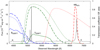 |
Fig. 1 Mean spectrum of HE 1136-2304 based on the observations performed with the SALT telescope together with the effective areas of the Swift B and V bandpass curves (in units of cm2 divided by 100) (solid lines); the Bochum B, V, and NB670 filter curves (dashed lines); and the MONET B, V, and R filter curves (dotted lines). |
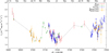 |
Fig. 2 Combined B-band continuum light curve (Swift, SALT, MONET, VYSOS-16, BEST II) calibrated with respect to the Swift data from 2014 to 2016. The time stamps at the top indicate the first day of the month. |
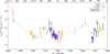 |
Fig. 3 Combined V -band continuum light curve (Swift, SALT, MONET, VYSOS-16, BEST II) calibrated with respect to the Swift data from 2014 to 2016. The time stamps at the top indicate the first day of the month. |
3.2 Host galaxy contribution to the optical continuum flux
Figure 6 displays the DSS1 image of HE 1136-2304 (Scale: 2 × 2 arcmin; pixel size 1.7 arcsec) as well as a B-V two-color image (bottom) based on VYSOS 16 data. The nucleus of HE 1136-2304 is surrounded by a spiral or S0 host galaxy; the radial profile of the surface brightness shows a central bulge structure and an extended disk structure in the DSS1 image. Some asymmetry of the outer isophotes might be connected with the object located to the east at a distance of 12 arcsec.
The observed flux of the variable AGN component is contaminated by the flux contribution of the host galaxy. The relative contribution of the host galaxy in the individual bands differs since the central nonthermal component has a different flux distribution from the stellar component of the host galaxy. Furthermore, the flux contribution of the host galaxy depends on the size of the aperture. In addition, we compare the accuracy and the results based on the photometric observations taken with Swift on the one hand and spectroscopic observations taken with SALT on the other hand. These photometric and spectroscopic observations were carried out with different apertures. All other photometric data were intercalibrated with respect to the absolute fluxes of Swift. Finally, we compare our results with those of Parker et al. (2016). Their results are based on only two spectra obtained in 1993 and 2014 and taken with different instruments and apertures.
We estimate the relative contribution of the constant host galaxy flux by means of the flux variation gradient (FVG) method (Choloniewski 1981; Winkler et al. 1992; Haas et al. 2011; Ramolla et al. 2015). This method disentangles the varying AGN flux in our aperture from the constant host galaxy contribution. We obtained B and V flux values of HE 1136-2304 based on the 5″ aperture of the Swift UVOT. Furthermore, we derived B-, V -, and R-band fluxes for the SALT spectra by convolving them with the B, V, and R filter curves (IRAF task sbands). We measured the fluxes at wavelengths close to the maxima of the filter curves (B-band filter: 4300 Å; V -band filter: 5400 Å; R-band filter: 6100 Å)with widths of a few hundred Å. In this way we excluded the contribution of emission lines in the spectra (see Fig. 1). These B, V, and R values are presented in Table 3.
Figures 7 and 8 show the B versus V and B versus R fluxes (black solid circles) of HE 1136-2304 based on the SALT spectra (aperture: 2 × 2 arcsec). The blue dashed line gives the best linear fit to the B versus V and B versus R fluxes. The black solid lines cover the upper and lower standard deviations of the interpolated AGN slope. The red dashed lines give the range of host slopes for nearby AGN as determined by Sakata et al. (2010). The intersection point between the AGN and host galaxy slopes gives the host galaxy fluxes in the B, V, and R bands. The gray lines indicate these B, V, and R values of the host galaxy.
Based on the intersection in the two figures, we derive a B-band flux of 0.27 mJy for the host galaxy contribution (mean of 0.25 and 0.29 mJy). The corresponding values are 0.57 mJy for the V band and 0.85 mJy for the R band. Our derived flux values for the contribution of the host galaxy in the B- and R-band spectra are 15% higher than those derived in Parker et al. (2016). The new values are of higher confidence. They are based on spectra taken under identical conditions at 21 epochs. Parker et al. (2016) used only two spectra taken with different apertures. Figure 9 shows the B versus V flux variations based on the Swift photometric data taken with a 12 arcsec aperture.
Once we know the integrated flux values of the host galaxy plus AGN as well as the host galaxy contribution, we can derive the AGN flux contribution in the individual bands. All these values are listed in Table 4. We present these values separately for the measurements based on the SALT spectra (based on the smaller aperture) and for the Swift data (based on the larger aperture). Furthermore, we give all these flux values in units of mJy and in units of 10−15 erg s−1 cm−2 Å−1 with the conversion formula
 (1)
(1)
where FmJy,λ is the flux in units of mJy, F the flux in units of 10−15 erg s−1 cm−2 Å−1, and λ the wavelength in Å.
The derived host galaxy fluxes in the B and V bands (based on the Swift data) are a factor two higher than those based on the SALT spectra because the larger extraction area of the Swift UVOT (10 arcsec diameter) collects more flux of the extended host galaxy than the SALT spectra do (2 × 2 arcsec only). However, the mean AGN fluxes derived on the basis of the SALT spectra are similar to those based on the Swift UVOT data (last three rows in Table 4). The AGN contribution based on the SALT spectra corresponds to 60%, 51%, and 41% in the B, V, and R band, respectively. The AGN contributionin the Swift UVOT B and V band decreases to 38% and 25%, respectively, because of their larger aperture.
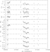 |
Fig. 4 Swift X-ray light curve from 2014 to 2016. The solid line at JD 2456841 marks the time of the XMM observation discussed in Parker et al. (2016). The observed 0.3–10 keV X-ray flux is given in units of 10−11 ergs s−1 cm−2. The X-ray count rates (CR), the X-ray photon index Γ of a simple power-law model, and the hardness ratios (HR) are also shown. The UVOT W2, M2, W1, U, B, and V magnitudes are given in the Vega system. |
Variability statistics based on the Swift continua (XRT, W2, M2, W1, U, B, V) and on the combined B and V light curves (Swift, SALT, MONET, Cerro Armazones) in units of 10−15 erg s−1 cm−2 Å−1 and 10−11 ergs s−1 cm−2 for the 0.3–10 keV X-ray data.
3.3 Swift inter-band correlation analysis and host galaxy contribution in the UV/optical bands
The Swift X-ray, UV, and optical light curves based on the variability campaign in 2015 are shown in Fig. 5. They all exhibit a similar variability pattern except for the V band, which exhibits no major variability amplitudes.
Based on these light curves we present the cross-correlation functions ICCF(τ) of all the Swift UVOT bands with respect to the XRT light curve in Fig. 10. In addition, we show the auto-correlation function (ACF) of the XRT band. We used the cross-correlation method as described in, e.g., Dietrich & Kollatschny (1995) and Kollatschny et al. (2014). Table 5 lists the maximum correlation coefficient rmax of the individual Swift bands with respect to the XRT band as well as the lags with respect to the XRT band. We derive the centroids of these ICCF, τcent, by using only the part of the CCF above 80% of the peak value. It has been shown by Peterson et al. (2003) that a threshold value of 0.8 rmax is generally a good choice. We determine the uncertainties of our cross-correlation results by calculating the cross-correlation lags many times using a model-independent Monte Carlo method known as flux redistribution/random subset selection (FR/RSS). This method was described by Peterson et al. (1998). The uncertainties correspond to 68% confidence levels.
The V -band light curve does not show any significant correlation with respect to the X-ray light curve (see Fig. 10). This might be caused by the nonthermal AGN contribution in the V band being less than 25% (see Table 4). Furthermore, the light distribution of the host galaxy is not exactly point-like, as seen in Fig. 6. Therefore, measurements made with a large aperture in the V band are more sensitive to small-scale deviations from an exact centering. By contrast, the X-ray and UV bands are dominated by the central nonthermal point source. Additionally, the V band is contaminated by the variable Hβ line (see Fig. 1).
Figure 11 shows the time delay of the Swift UV and optical bands with respect to the Swift X-ray light curve as a function of wavelength. The V band has been excluded here as it showed no correlation. The dashed line shows the most general fit to the data:
![Mathematical equation: \[ \uptau = b((\uplambda/\lambda_{0})^{c}-1) \]](/articles/aa/full_html/2018/10/aa32506-17/aa32506-17-eq9.png)
with λ0 = 25 Å. The b-valueand the power-law index c have been allowed to vary. First we determined the fit parameter b = 0.003 ± 0.020 light-days giving a hint on the size of the X-ray emitting region at λ0 = 25 Å (corresponding to λpivot of XRT filter). Afterwards we kept b fixed and calculated the exponent c. The best fit to the data gives c = 1.3 ± 0.1. This value is consistent with a theoretically expected value c = 1.33 = 4/3 for an irradiated accretion disk (see discussion section).
The UV and optical spectral energy distribution of HE 1136-2304 based on our Swift data taken in 2015 is presented in Fig. 12 with black symbols. The red open circles show the contribution of the host galaxy in the individual bands. The host contribution in the B and V bands is based on the FVG analysis (Sect. 3.2). We calculated the contribution of the host galaxy in the UV bands by scaling an Sb spectrum (Kinney et al. 1996) with respect to the B and V fluxes of the host galaxy. The AGN flux in the individual bands has been determined by subtracting the flux of the host galaxy from the observed flux. The blue filled squares in Fig. 12 give the AGN flux contribution in the individual Swift bands. Knowing the AGN flux contribution in the individual Swift bands, we can derive the pure fractional variations in those bands. We present the fractional variations of the UV and optical continuum bands recorded with Swift in 2015 as a function of wavelength in Fig. 13. The contribution of the host galaxy flux has been subtracted from the individual filter bands. We then add (in red) the fractional variations in the B and V bands on basis of our measurements with the different telescopes in 2015. There is a clear trend of increasing fractional variation of the AGN towards the UV. The dashed line shows a general fit to the data with a value c = 0.84.
We present the fractional variation of the X-ray band together with the fractional variations of the UV/optical bands in Fig. 14. The fractional variations in X-rays are the strongest (as seen in Table 2). However, the fractional variations in X-rays do not follow the same trend as seen for the fractional variations in the UV and optical bands. An extrapolation of the fit in the UV and optical bands does not line up with the X-ray observations. This is an indication that the origin of theX-ray continuum emission is not connected in a simple way with the origin of the UV/optical emission (see Sect. 4.2).
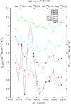 |
Fig. 5 Combined optical, UV, and X-ray light curves taken with the Swift satellite for the dedicated campaign in 2015. |
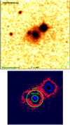 |
Fig. 6 Top: DSS1 image of HE 1136-2304. Scale: 2 × 2 arcmin. North is to the top, east to the left. Bottom: enlarged B-V two color image based on VYSOS 16 data. The small green circle has r =3.′′75, indicating that the aperture used for the OCA photometry is sufficiently small to be not contaminated by the star located about 20′′ in the NW and the faint source in the E. The large green circle with r =10′′ as labeled indicates the projected distance to the eastern source. |
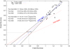 |
Fig. 7 Flux variations (B vs. V) of HE 1136-2304 based on the SALT spectra. The blue dashed line is the best linear fit to the B vs. V fluxes. The black solid lines cover the upper and lower standard deviations of the interpolated AGN slope. The red dashed lines give the range of host slopes as determined by Sakata et al. (2010). The gray lines indicate the central B and V values of the host galaxy. Listed are the B and V flux values (in units of mJy and 10−15 erg s−1 cm−2 Å−1) for the combined mean host galaxy+AGN flux, for the host galaxy flux, and for the mean AGN flux. |
B, V, and R flux values based on Salt spectra.
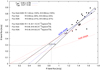 |
Fig. 8 Flux variations (B vs. R) of HE 1136-2304 based on the SALT spectra. The blue dashed line presents the best linear fit to the B vs. R fluxes. The black solid lines cover the upper and lower standard deviations of the interpolated AGN slope. The red dashed lines show the range of host slopes. The gray lines indicate the B and R values of the host galaxy. The B and R flux values are listed as in Fig. 7. |
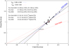 |
Fig. 9 Flux variations (B vs. V) of HE 1136-2304 based on the photometric Swift data. The blue dashed line presents the best linear fit to the B vs. V fluxes. The black solid lines cover the upper and lower standard deviations of the interpolated AGN slope. The red dashed lines show the range of host slopes. The gray lines indicate the central B and V values of the host galaxy. The B and V flux values are listed as in Fig. 7. |
3.4 Spectral type changes and long-term variability of HE 1136-2304
The first spectrum of HE 1136-2304 was taken in 1993 (Reimers et al. 1996). At that time no broad Hβ emission line component was present in the spectrum. Only a faint broad Hα component was visible. Therefore, this galaxy was of nearly Seyfert 2 (1.95) type in 1993. Another spectrum of HE 1136-2304 was obtained on 2002 May 16 as part of the 6dF Galaxy Survey (Jones et al. 2004). At this time HE 1136-2304 was of the same spectral AGN type as it was nine years earlier. The AGN type had changed to Seyfert 1.5 when we took an optical spectrum in 2014 July (Parker et al. 2016). This happened together with an increase in the optical continuum flux and with a strong increase in X-ray flux.
In Fig. 15 the spectra of HE 1136-2304 taken in 1993, 2002, 2014, 2015, 2016, and 2017 are shown to present line profile changes. The spectra are shifted by a constant with respect to each other. Figures 16 and 17 show the Hβ and Hα spectral regions in more detail. The mean spectrum for 2015 is based on the variability campaign carried out in 2015. We will present details of this campaign in a separate publication. The spectrum shown for 2016 is the mean of two spectra taken in May 2016. The strong broad component in the Hβ line profile that appeared in 2014 remained there for the subsequent years until 2017. No major profile changes occurred. HE 1136-2304 remained a Seyfert 1.5 type.
We compared the spectral variations of the data from 1993 to 2017 with the variability behavior in the optical and X-ray continuum. Figure 18 shows the X-ray and optical B-band continuum variations from 2014 to 2016. The long-term trends for 1993 to 2017 are presented in Fig. 19. The Swift X-ray data and the ROSAT upper limit for 1990 are presented in red (axis label on the left side). The optical continuum variations are given in blue.
We scaled the amplitude of the optical light curve with respect to the X-ray light curve. The scaling has been carried out with regard to nearly simultaneous observations in the optical and X-rays in 2014 July and for the combined variability campaign in2015. The axis label for the blue continuum is given on the right side. Dramatic continuum variations in X-rays and in the optical occurred between 2014 and 2016. The optical continuum closely follows the X-ray flux. HE 1136-2304 was in a low state in X-rays and in the optical before 2000.
B, V, and R values (in units of mJy and 10−15 erg s−1 cm−2 Å−1) for the combined host galaxy+AGN fluxes as well as for the host galaxy and AGN fluxes alone.
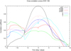 |
Fig. 10 Cross-correlation functions ICCF(τ) of the Swift bands UVW2, UVM2, UVW1, U, B, and V with respect to the XRT light curve. Also shown is an auto-correlation function (ACF) of the XRT band. |
4 Discussion
One of the main goals of our optical, UV, and X-ray variability campaign was to investigate the variability behavior of the changing-look AGN HE 1136-2304 subsequent to the outburst in 2014 July. Our campaigns in X-rays and UV, and at optical wavelengths lasted for two and three years, respectively.
A strong and sudden outburst in AGN can in principle be caused by three different events: gravitational lensing, a tidal disruption event (TDE), or major changes in the accretion process. Light curves caused by a lensing effect should exhibit a characteristic smooth, single-peaked shape (e.g., Bruce et al. 2017). A tidal disruption event is characterized by a sudden dramatic rise in luminosity and a steady decline to quiescence on timescales of months to years (Rees 1988). Some candidates for TDEs in X-rays, UV, and optical bands have been presented by, e.g., Komossa & Bade (1999), Gezari et al. (2008), and Holoien et al. (2016). However, the variability pattern of HE 1136-2304 following the outburst in 2014 shows various outbursts on timescales of days to months typical for “ordinary” AGN variability (see Figs. 2–4). Therefore, we can rule outa micro lensing or tidal disruption event as the cause of the observed variability pattern seen in HE 1136-2304.
Swift inter-band correlation coefficients (rmax) and lags (τ).
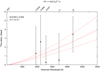 |
Fig. 11 Time delay of the Swift UV and optical bands with respect to the Swift XRT light curve as a function of the wavelength of the Swift bands. The V band has been excluded as it showed a very low correlation coefficient. The dashed line shows the best fit to the data. The dotted lines give the error of the exponent c. |
4.1 Optical continuum variability in HE 1136-2304
HE 1136-2304 shows no systematic long-term trends in the continuum light curves (see Fig. 2) since the start of our variability campaign in 2014 July. After two years the light curve reaches approximately the same flux level as in 2014 July, while showing unsystematic flux variations down to about 50% in between.
One way to measure the strength of the variability in AGN is to determine their fractional variation Fvar. The fractional variation depends on the duration of the monitoring campaign, on the examined wavelength, and on the (accurate) decomposition of the host galaxy contribution. A typical value for the fractional variation Fvar of the continuum at 5100 Å is 0.05 to 0.15 for variability periods of 6–12 months: e.g., NGC 5548 (Peterson et al. 2002; Fausnaugh et al. 2016), 3C 120 (Kollatschny et al. 2014). For variability campaigns over longer periods, typical Fvar continuum values at 5100 Å are from 0.1to 0.25: e.g., NGC 5548 (Peterson et al. 2002), Ark 564 (Shapovalova et al. 2012), Mrk 110 (Kollatschny et al. 2001), or 3C 120 (Kollatschny et al. 2014), and a collection of many AGN in Kollatschny & Zetzl 2006. This higher Fvar value is caused by the irregular variations of AGN on longer timescales. There is a higher probability for observing stronger variability amplitudes when monitoring over longer periods of time. We determined optical Fvar values of 0.11 (5360 Å) and 0.14 (4570 Å) for our campaign in 2015 (based on the SALT spectra). Our value of 0.11 for Fvar indicates that the continuum variations of HE 1136-2304 were equal to or even stronger than other AGN, in particular after correcting for the flux contribution of the host galaxy.
For a more detailed inspection of the AGN variability, the contribution of the host galaxy starlight should be subtracted before comparing the amplitudes of different AGN. The relative contribution of the host galaxy flux is quite different in spectroscopic and photometric data (see Table 4). The typical contribution of the host galaxy is larger if it is based on broadband photometry because the typical aperture for broadband photometry is larger than that for spectral photometry. One way to estimate the contribution of the host galaxy is to create nucleus-free images of the AGN based on HST images (e.g., Bentz et al. 2009) or by decomposition of the observed AGN spectra (e.g., Barth et al. 2015). Typical values for the relative host galaxy flux contribution are in the order of 20% to 60% in optical AGN spectra (see Fig. 4 in Barth et al. 2015). The flux variation gradient (FVG) method (Choloniewski 1981; Winkler et al. 1992; Haas et al. 2011; Ramolla et al. 2015) is another way to estimate the relative contribution of the host galaxy flux to the variable continuum flux. A typical value for the relative contributions of the host galaxy flux is on the order of 50% (e.g., Haas et al. 2011) for broadband photometry. The contribution of the host galaxy flux in HE 1136-2304 amounts to 50% (for spectrum photometry) and to 75% (for broadband photometry) in the V band. Therefore, the variability amplitude in HE 1136-2304 remains quite high in comparison to other AGN after subtraction of the host galaxy flux.
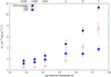 |
Fig. 12 Mean UV and optical spectral energy distribution of HE 1136-2304 based on the Swift data taken in 2015 (black filled circles). The red open circles and the blue squares indicate the contributions of the host galaxy and the AGN, respectively. |
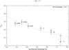 |
Fig. 13 Fractional variations of the UV and optical continuum bands derived from the Swift data in 2015 as a function of wavelength. Furthermore, the B and V band measurements based on the photometric data taken in 2015 have been added. The contribution of the host galaxy has been subtracted in all cases. The dashed line shows a general fit with an exponent c = 0.84. |
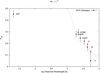 |
Fig. 14 Fractional variations of the X-ray, UV, and optical continuum bands measured from the Swift data in 2015 as a function of wavelength. |
4.2 Comparison of X-ray variations against UV/optical variations
The time delays of the individual Swift UV/optical light curves with respect to the Swift X-ray light curve are presented in Fig. 11. There is a trend that the UV/optical light curves at higher frequencies show shorter delays. A general fit to the data in Fig. 11 resulted in a value of 0.003 ± 0.020 light-days for the fit parameter b in  , with λ0 = 25Å.
This functional form of τ has been discussed before by Edelson et al. (2015) and Fausnaugh et al. (2016) in the context of the Swift and HST reverberation mapping campaign on NGC 5548. The value of b gives an estimate of the size of the X-ray emitting region. A value of 0.020 light-days (based on the error of the b value) corresponds to 5.1 × 10¹¹ m. We can compare this size with the Schwarzschild radius for a central black hole mass of M = 4 × 10⁷M⊙ (Kollatschny et al. 2018): 1.2 × 10¹¹ m. This indicates that the X-ray emission originates at a distance of a few Schwarzschild radii from the center which is consistentwith the last stable orbit of a Schwarzschild black hole.
The second parameter we derived from the general fit shown in Fig. 11 is the parameter c = 1.3 ± 0.1. This value is close to a theoretically expected value c = 1.33 = 4/3 for an irradiated accretion disk where the geometrically thin, optically thick accretion disk is hotter in the inner radii and cooler in the outer radii (e.g., Cackett et al. 2007; Edelson et al. 2015). The optical continuum is delayed by about three light-days with respect to the X-ray variations. Similar delays of approximately 3 to 4 light-days of the optical continuum bands with respect to the UV/X-ray bands have also been seen in Swift variability campaigns of NGC 2617 (Shappee et al. 2014) and NGC 5548 (Fausnaugh et al. 2016). A further indicationthat the optical continuum in HE 1136-2304 is delayed with respect to the ionizing continuum will be presented ina future paper (Kollatschny et al. 2018) where we show that the outer line wings, for example in Hβ, respond faster than the adjacent optical continuum.
As shown in Fig. 13, the fractional variability Fvar of the continuum bands is a function of their wavelength. The variations are stronger at shorter wavelength bands. This means that the strengthof the fractional variability can be considered as a proxy for the distance of the continuum emitting region with respect to the center. Similar to the time delay of the individual continuum bands, we can test whether a power-law model Fvar = a × λ−c is consistent with the observations. The optimal c value c = 0.84 we found is close to a simple power law with c = 1: Fvar = a × λ−1. Furthermore, as shown in Fig. 14, the fractional variations in the X-ray band are 50% stronger than those in the UV bands. However, the magnitude of the fractional variation in X-rays is not simply a continuation of the general trend seen in the UV and optical bands. This indicates that the observed X-ray emission does not exactly follow the same trend as the UV/optical emission. The UV/optical continuum emission is generally associated with blackbody emission from the accretion disk (e.g., Hubeny et al. 2001).
We tested whether the observed trend of the fractional variability in the UV/optical bands of HE 1136-2304 is present in other galaxies as well, for example in NGC 5548. An extensive variability campaign of NGC 5548 has been carried out in 2014 (Edelson et al. 2015; Fausnaugh et al. 2016). Their fractional variability data of NGC 5548 are shown in Fig. 20.
A fit with Fvar = a × λ−c and c = 0.74 perfectly matches the observations of NGC 5548. This c value is close to the optimal c value of 0.84 we found for HE 1136-2304. A comparison of the fractional variations of NGC 5548 (Fig. 20) with those of HE 1136-2304 (Fig. 13) shows that the variations in the UV/X-ray bands of HE 1136-2304 are stronger by a factor of 2.3.
However, there are different trends when comparing the variably pattern in X-rays and in the UV/optical observed in HE 1136-2304 with those seen in NGC 5548 (Edelson et al. 2015). The UV/optical light curves of HE 1136-2304 show the same pattern as the X-ray light curve, while this is not the case in NGC 5548 (Edelson et al. 2015). Furthermore, in HE 1136-2304 the strongest variability is observed in X-rays, while this is not the case in NGC 5548. Edelson et al. (2015) suspected that the X-ray flux may not drive the UV/optical light curves in NGC 5548 because of his findings. Such a statement cannot be made for HE 1136-2304 based on its light curves.
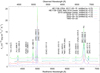 |
Fig. 15 Optical spectra of HE 1136-2304 for the epochs 1993, 2002, 2014, 2017, as well as mean spectra for 2015 and 2016. |
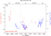 |
Fig. 18 Optical (blue) and X-ray (red) light curve from 2014 to 2016. The upper limit of the X-ray flux in 1990 (ROSAT) is shown by a horizontal dashed line. |
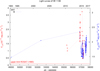 |
Fig. 19 Long-term optical (blue) and X-ray (red) light curves of HE 1136-2304 from 1993 to 2017. The Swift X-ray data and the upper X-ray limit in 1990 based on ROSAT is presented in red (left axis label). The B-band data are scaled with respect to the X-ray data, and are shown in blue (right axis label). |
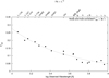 |
Fig. 20 Fit to the fractional variations in the UV and optical bands of an extensive variability campaign of NGC 5548 (with c = 0.74). The data are from Fausnaugh et al. (2016). |
4.3 Comparison of optical spectral changes with continuum variations in HE 1136-2304
Early optical spectra of HE 1136-2304 were taken in 1993 and 2002. At that time, it was of nearly Seyfert 2 (1.95) type. We took a spectrum in 2014 July. The spectral type of HE 1136-2304 had changed to be of Seyfert 1.5. Since then the spectral type remained the same (see Figs. 15–17). There are no major variations present in the Balmer line profiles for the period from 2014 to the present. However, the optical and X-ray continua varied a lot at the same time (see Fig. 18).
It has been discussed by Parker et al. (2016) whether the outburst seen in 2014 was caused by a flare due to a stellar disruption event (e.g., Komossa & Bade 1999). In that case we would have expected a general decline in the continuum flux of HE 1136-2304 over time. However, the observed long-term behavior with repeated phases of decreasing and increasing continuum flux between 2014 and 2017 contradicts this scenario.
On the other hand, Elitzur et al. (2014) present a model in which the broad-line spectral evolution is connected with the AGN luminosity. This might be controlled by the accretion rate onto the central black hole. The long-term variations ofHE 1136-2304 from 1993 to 2014 support this model: the X-ray flux increased by a factor of more than ten. The B-band continuum flux (without correction for the host galaxy contribution) increased by more than 60%, and the spectral type changed from a nearly Seyfert 2 type to a Seyfert 1.5 type. A similar scenario, but with decreasing continuum flux, has been found for Fairall 9. The continuum flux dropped to 20% of its original flux in 1978, and its spectral type changed from a quasar/Seyfert 1 type to a Seyfert 1.95 type within 6 years (Kollatschny & Fricke 1985). Spectral variations of this kind generally occur on timescales of years.
However, the spectral type variations seem not to follow the continuum intensity variations on shorter timescales (weeks to months). In 2015, HE 1136-2304 varied in the X-rays by a factor of eight within two months (see Fig. 18), whereas the broad-line profiles varied only marginally over the period from 2014 to 2017 (see Fig. 15). A detailed discussion of the spectral variability campaign carried out in 2015 will be presented in a separate paper (Kollatschny et al. 2018).
5 Summary
We present results of an optical, UV, and X-ray monitoring campaign of the changing-look AGN HE 1136-2304 carried out from 2014 to 2017. This campaign took place after a continuum outburst in the optical and X-rays in 2014 July connected to a spectral change from a Seyfert 1.95 to a Seyfert 1.5 type. Our findings can be summarized as follows:
- (1)
The optical, UV, and X-ray continuum light curves show the same variability pattern. The amplitude decreases with increasing wavelength. It varies by a factor of eight in X-rays, by a factor of four in the UV, and by a factor of two in the optical continuum between 2014 and 2016. The amplitude in the optical increases by a factor of three after correction for the host galaxy contribution.
- (2)
No general trend was visible in the variability pattern. This rules out that the outburst in 2014 was caused by gravitational lensing or by a tidal disruption event. In these cases we would have expected a general decrease in the emitted continuum flux.
- (3)
The optical B-band continuum light curve is delayed by about three days with respect to the X-ray light curve.
- (4)
The spectral type of HE 1136-2304 remained as Seyfert 1.5 between 2014 and 2017 despite its strong continuum variations at the same time.
Acknowledgements
We are thankful to the late Neil Gehrels for approving our ToO requests. We also thank the Swift team for performing the ToO observations. This research has made use of the XRT Data Analysis Software (XRTDAS) developed under the responsibility of the ASI Science Data Center (ASDC), Italy. This research has made use of the NASA/IPAC Extragalactic Database (NED) which is operated by the Jet Propulsion Laboratory, Caltech, under contract with the National Aeronautics and Space Administration. This work has been supported by the DFG grants Ha 3555/12-1, Ko 857/32-2, and Ko 857/33-1.
Appendix A Additional tables
Swift monitoring: optical, UV flux densities.
Swift monitoring: X-ray data.
B and V -band fluxes.
XRT and UVOT monitoring observation log.
Log of photometric observations with MONET/North (N) and MONET/South (S).
Log of photometric observations with VYSOS 16 (V 16) and BEST II (B II).
References
- Arnaud, K. A. 1996, ASP Conf. Ser., 101, 17 [Google Scholar]
- Barth, A. J., Bennert, V. N., Canalizo, G., et al. 2015, ApJS, 217, 26 [NASA ADS] [CrossRef] [Google Scholar]
- Bentz, M. C., Peterson, B. M., Netzer, H., Pogge, R. W., & Vestergaard, M. 2009, ApJ, 697, 160 [Google Scholar]
- Breeveld, A. A., Curran, P. A., Hoversten, E. A., et al. 2010, MNRAS, 406, 1687 [NASA ADS] [Google Scholar]
- Bruce, A., Lawrence, A., MacLeod, C., et al. 2017, MNRAS, 467, 1259 [NASA ADS] [Google Scholar]
- Burrows, D. N, Hill, J. E., Nousek, J. A., et al. 2005, Space Sci. Rev., 120, 165 [NASA ADS] [CrossRef] [Google Scholar]
- Cackett, E. M., Horne, K., & Winkler, H. 2007, MNRAS, 380, 669 [NASA ADS] [CrossRef] [Google Scholar]
- Cardelli, J. A., Clayton, G. C., & Mathis, J. S. 1989, ApJ, 345, 245 [NASA ADS] [CrossRef] [Google Scholar]
- Cash, W. 1979, ApJ, 228, 939 [NASA ADS] [CrossRef] [Google Scholar]
- Choloniewski, J. 1981, Acta Astron., 31, 293 [NASA ADS] [Google Scholar]
- Collin-Souffrin, S., Alloin, D., & Andrillat, Y. 1973, A&A, 22, 343 [NASA ADS] [Google Scholar]
- Denney, K. D., De Rosa, G., Croxall, K., et al. 2014, ApJ, 796, 134 [NASA ADS] [CrossRef] [Google Scholar]
- Dietrich, M., & Kollatschny, W. 1995, A&A, 303, 405 [NASA ADS] [Google Scholar]
- Edelson, R., Turner, T. J., Pounds, K., et al. 2002, ApJ, 568, 610 [NASA ADS] [CrossRef] [Google Scholar]
- Edelson, R., Gelbord, J. M. Horne, K., et al. 2015, ApJ, 806, 129 [NASA ADS] [CrossRef] [Google Scholar]
- Elitzur, M., Ho, L. C., & Trump, J. R. 2014, MNRAS, 438, 3340 [NASA ADS] [CrossRef] [Google Scholar]
- Fausnaugh, M. M., Denney, K. D., Barth, A. J., et al. 2016, ApJ, 821, 56 [NASA ADS] [CrossRef] [Google Scholar]
- Fitzpatrick, E. L. 1999, PASP, 111, 63 [NASA ADS] [CrossRef] [Google Scholar]
- Gehrels, N., Chincarini, G., Giommi, P., et al. 2004, ApJ, 611, 1005 [NASA ADS] [CrossRef] [Google Scholar]
- Gezari, S., Basa, S., Martin, D. C., et al. 2008, ApJ, 676, 944 [NASA ADS] [CrossRef] [Google Scholar]
- Grupe, D., Thomas, H.-C., & Beuermann, K. 2001, A&A, 367, 470 [NASA ADS] [CrossRef] [EDP Sciences] [Google Scholar]
- Grupe, D., Komossa, S., Leighly, K. M., & Page, K. L. 2010, ApJS, 187, 64 [NASA ADS] [CrossRef] [Google Scholar]
- Guainazzi, M. 2002, MNRAS, 329, L13 [NASA ADS] [CrossRef] [Google Scholar]
- Haas, M., Chini, R., Ramolla, M., et al. 2011, A&A, 535, A73 [NASA ADS] [CrossRef] [EDP Sciences] [Google Scholar]
- Hill, J. E., Burrows, D. N., Nousek, J. A., et al. 2004, Proc. SPIE, 5165, 217 [NASA ADS] [CrossRef] [Google Scholar]
- Holoien, T. W.-S., Kochanek, C. S., Prieto, J. L., et al. 2016, MNRAS, 455, 2918 [NASA ADS] [CrossRef] [Google Scholar]
- Hubeny, I., Blaes, O., Krolik, J. H., & Agol, E. 2001, ApJ, 559, 680 [NASA ADS] [CrossRef] [Google Scholar]
- Jones, D. H., Saunders, W., Colless, M., et al. 2004, MNRAS, 355, 747 [NASA ADS] [CrossRef] [Google Scholar]
- Kabath, P., Erikson, A., Rauer, H., et al. 2009, A&A, 506, 569 [NASA ADS] [CrossRef] [EDP Sciences] [Google Scholar]
- Kalberla, P. M. W., Burton, W. B., Hartmann, D., et al. 2005, A&A, 440, 775 [NASA ADS] [CrossRef] [EDP Sciences] [Google Scholar]
- Kinney, A. L., Calzetti, D., Bohlin, R. C., et al. 1996, ApJ, 467, 38 [NASA ADS] [CrossRef] [Google Scholar]
- Kollatschny, W. 2003, A&A, 407, 461 [NASA ADS] [CrossRef] [EDP Sciences] [Google Scholar]
- Kollatschny, W., & Fricke, K. J. 1985, A&A, 146, L11 [NASA ADS] [Google Scholar]
- Kollatschny, W., & Zetzl, M. 2006, A&A, 454, 459 [NASA ADS] [CrossRef] [EDP Sciences] [Google Scholar]
- Kollatschny, W., & Zetzl, M. 2010, A&A, 522, A36 [NASA ADS] [CrossRef] [EDP Sciences] [Google Scholar]
- Kollatschny, W., Bischoff, K., & Dietrich, M. 2000, A&A, 361, 901 [NASA ADS] [Google Scholar]
- Kollatschny, W., Bischoff, K., Robinson, E. L., Welsh, W. F., & Hill, G. J., 2001, A&A, 379, 125 [NASA ADS] [CrossRef] [EDP Sciences] [Google Scholar]
- Kollatschny, W., Ulbrich, K., Zetzl, M., Kaspi, S., & Haas, M. 2014, A&A, 566, A106 [NASA ADS] [CrossRef] [EDP Sciences] [Google Scholar]
- Kollatschny, W., Ochmann, M. W., Zetzl, M., et al. 2018, A&A, in press, DOI: 10.1051/0004-6361/201833727 [Google Scholar]
- Komossa, S., & Bade, N. 1999, A&A, 343, 775 [NASA ADS] [Google Scholar]
- Komossa, S., Zhou, H., Wang, T., et al. 2008, ApJ, 678, L13 [NASA ADS] [CrossRef] [Google Scholar]
- LaMassa, S. M., Cales, S., Moran, E. C., et al. 2015, ApJ, 800, 144 [NASA ADS] [CrossRef] [Google Scholar]
- Landolt, A. U. 2009, AJ, 137, 4186 [NASA ADS] [CrossRef] [Google Scholar]
- Macleod, C. L., Ross, N. P., Lawrence, A., et al. 2016, MNRAS, 457, 389 [NASA ADS] [CrossRef] [Google Scholar]
- Patat, F., Moehler, S., O’Brien, K., et al. 2011, A&A, 527, A91 [NASA ADS] [CrossRef] [EDP Sciences] [Google Scholar]
- Park, T., Kashyap, V. L., Siemiginowska, A., et al. 2006, ApJ, 652, 610 [NASA ADS] [CrossRef] [Google Scholar]
- Parker, M. L., Komossa, S., Kollatschny, W., et al. 2016, MNRAS, 461, 1927 [NASA ADS] [CrossRef] [Google Scholar]
- Pei, L., Fausnaugh, M. M., Barth, A. J., et al. 2017, ApJ, 837, 131 [NASA ADS] [CrossRef] [Google Scholar]
- Penston, M. V., & Perez, E. 1984, MNRAS, 211, 33 [Google Scholar]
- Peterson, B. M., Wanders, I., Bertram, R., et al. 1998, ApJ, 501, 82 [NASA ADS] [CrossRef] [Google Scholar]
- Peterson, B. M., Berlind, P., Bertram, R., et al. 2002, ApJ, 581, 197 [NASA ADS] [CrossRef] [Google Scholar]
- Peterson, B. M., Ferrarese, L., Gilbert, K. M., et al. 2004, ApJ, 613, 682 [NASA ADS] [CrossRef] [Google Scholar]
- Poole, T. S., Breeveld, A. A., Page, M. J., et al. 2008, MNRAS, 383, 627 [NASA ADS] [CrossRef] [Google Scholar]
- Pozo Nuñez, F., Ramolla, M., Westhues, C., et al. 2015, A&A, 576, A73 [NASA ADS] [CrossRef] [EDP Sciences] [Google Scholar]
- Ramolla, M., Drass, H., Lemke, R., et al. 2013, Astron. Nachr., 334, 1115 [NASA ADS] [CrossRef] [Google Scholar]
- Ramolla, M., Pozo Nuñez, F., Westhues, C., Haas, M., & Chini, R. 2015, A&A, 581, A93 [NASA ADS] [CrossRef] [EDP Sciences] [Google Scholar]
- Rees, M. 1988, Nature, 333, 523 [NASA ADS] [CrossRef] [Google Scholar]
- Reimers, D., Koehler, T., & Wisotzki, L. 1996, A&AS, 115, 235 [NASA ADS] [Google Scholar]
- Rodríguez-Pascual, P. M., Alloin, D., Clavel, J., et al. 1997, ApJS, 110, 9 [NASA ADS] [CrossRef] [Google Scholar]
- Roming, P. W. A., Kennedy, T. E., Mason, K. O, et al. 2005, Space Sci. Rev., 120, 95 [NASA ADS] [CrossRef] [Google Scholar]
- Roming, P. W. A., Koch, T. S., Oates, S. R., et al. 2009, ApJ, 690, 163 [NASA ADS] [CrossRef] [Google Scholar]
- Runnoe, J. C., Cales, S., Ruan, J. J., et al. 2016, MNRAS, 455, 1691 [NASA ADS] [CrossRef] [Google Scholar]
- Sakata, Y., Minezaki, T., Yoshii, Y., et al. 2010, ApJ, 711, 461 [NASA ADS] [CrossRef] [Google Scholar]
- Schlafly, E. F., & Finkbeiner, D. P. 2011, ApJ, 737, 103 [NASA ADS] [CrossRef] [Google Scholar]
- Schlegel, D. J., Finkbeiner, D. P., & Davis, M. 1998, ApJ, 500, 525 [NASA ADS] [CrossRef] [Google Scholar]
- Shapovalova, A. I., Popović, L. Ć, Burenkov, A. N., et al. 2010, A&A, 517, A42 [NASA ADS] [CrossRef] [EDP Sciences] [Google Scholar]
- Shapovalova, A. I., Popović, L. Ć, Burenkov, A. N., et al. 2012, ApJS, 202, 10 [NASA ADS] [CrossRef] [Google Scholar]
- Shappee, B. J., Prieto, J. L., Grupe, D., et al. 2014, ApJ, 788, 48 [NASA ADS] [CrossRef] [Google Scholar]
- Winkler, H., Glass, I. S., van Wyk, F., et al. 1992, MNRAS, 257, 659 [NASA ADS] [Google Scholar]
- Wright, E. L. 2006, PASP, 118, 1711 [NASA ADS] [CrossRef] [Google Scholar]
All Tables
Variability statistics based on the Swift continua (XRT, W2, M2, W1, U, B, V) and on the combined B and V light curves (Swift, SALT, MONET, Cerro Armazones) in units of 10−15 erg s−1 cm−2 Å−1 and 10−11 ergs s−1 cm−2 for the 0.3–10 keV X-ray data.
B, V, and R values (in units of mJy and 10−15 erg s−1 cm−2 Å−1) for the combined host galaxy+AGN fluxes as well as for the host galaxy and AGN fluxes alone.
All Figures
|
Fig. 1 Mean spectrum of HE 1136-2304 based on the observations performed with the SALT telescope together with the effective areas of the Swift B and V bandpass curves (in units of cm2 divided by 100) (solid lines); the Bochum B, V, and NB670 filter curves (dashed lines); and the MONET B, V, and R filter curves (dotted lines). |
| In the text | |
|
Fig. 2 Combined B-band continuum light curve (Swift, SALT, MONET, VYSOS-16, BEST II) calibrated with respect to the Swift data from 2014 to 2016. The time stamps at the top indicate the first day of the month. |
| In the text | |
|
Fig. 3 Combined V -band continuum light curve (Swift, SALT, MONET, VYSOS-16, BEST II) calibrated with respect to the Swift data from 2014 to 2016. The time stamps at the top indicate the first day of the month. |
| In the text | |
|
Fig. 4 Swift X-ray light curve from 2014 to 2016. The solid line at JD 2456841 marks the time of the XMM observation discussed in Parker et al. (2016). The observed 0.3–10 keV X-ray flux is given in units of 10−11 ergs s−1 cm−2. The X-ray count rates (CR), the X-ray photon index Γ of a simple power-law model, and the hardness ratios (HR) are also shown. The UVOT W2, M2, W1, U, B, and V magnitudes are given in the Vega system. |
| In the text | |
|
Fig. 5 Combined optical, UV, and X-ray light curves taken with the Swift satellite for the dedicated campaign in 2015. |
| In the text | |
|
Fig. 6 Top: DSS1 image of HE 1136-2304. Scale: 2 × 2 arcmin. North is to the top, east to the left. Bottom: enlarged B-V two color image based on VYSOS 16 data. The small green circle has r =3.′′75, indicating that the aperture used for the OCA photometry is sufficiently small to be not contaminated by the star located about 20′′ in the NW and the faint source in the E. The large green circle with r =10′′ as labeled indicates the projected distance to the eastern source. |
| In the text | |
|
Fig. 7 Flux variations (B vs. V) of HE 1136-2304 based on the SALT spectra. The blue dashed line is the best linear fit to the B vs. V fluxes. The black solid lines cover the upper and lower standard deviations of the interpolated AGN slope. The red dashed lines give the range of host slopes as determined by Sakata et al. (2010). The gray lines indicate the central B and V values of the host galaxy. Listed are the B and V flux values (in units of mJy and 10−15 erg s−1 cm−2 Å−1) for the combined mean host galaxy+AGN flux, for the host galaxy flux, and for the mean AGN flux. |
| In the text | |
|
Fig. 8 Flux variations (B vs. R) of HE 1136-2304 based on the SALT spectra. The blue dashed line presents the best linear fit to the B vs. R fluxes. The black solid lines cover the upper and lower standard deviations of the interpolated AGN slope. The red dashed lines show the range of host slopes. The gray lines indicate the B and R values of the host galaxy. The B and R flux values are listed as in Fig. 7. |
| In the text | |
|
Fig. 9 Flux variations (B vs. V) of HE 1136-2304 based on the photometric Swift data. The blue dashed line presents the best linear fit to the B vs. V fluxes. The black solid lines cover the upper and lower standard deviations of the interpolated AGN slope. The red dashed lines show the range of host slopes. The gray lines indicate the central B and V values of the host galaxy. The B and V flux values are listed as in Fig. 7. |
| In the text | |
|
Fig. 10 Cross-correlation functions ICCF(τ) of the Swift bands UVW2, UVM2, UVW1, U, B, and V with respect to the XRT light curve. Also shown is an auto-correlation function (ACF) of the XRT band. |
| In the text | |
|
Fig. 11 Time delay of the Swift UV and optical bands with respect to the Swift XRT light curve as a function of the wavelength of the Swift bands. The V band has been excluded as it showed a very low correlation coefficient. The dashed line shows the best fit to the data. The dotted lines give the error of the exponent c. |
| In the text | |
|
Fig. 12 Mean UV and optical spectral energy distribution of HE 1136-2304 based on the Swift data taken in 2015 (black filled circles). The red open circles and the blue squares indicate the contributions of the host galaxy and the AGN, respectively. |
| In the text | |
|
Fig. 13 Fractional variations of the UV and optical continuum bands derived from the Swift data in 2015 as a function of wavelength. Furthermore, the B and V band measurements based on the photometric data taken in 2015 have been added. The contribution of the host galaxy has been subtracted in all cases. The dashed line shows a general fit with an exponent c = 0.84. |
| In the text | |
|
Fig. 14 Fractional variations of the X-ray, UV, and optical continuum bands measured from the Swift data in 2015 as a function of wavelength. |
| In the text | |
|
Fig. 15 Optical spectra of HE 1136-2304 for the epochs 1993, 2002, 2014, 2017, as well as mean spectra for 2015 and 2016. |
| In the text | |
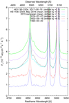 |
Fig. 16 Optical spectra of HE 1136-2304, as in Fig. 15, but showing the Hβ profiles in more detail. |
| In the text | |
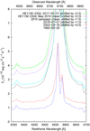 |
Fig. 17 Optical spectra of HE 1136-2304, as in Fig. 15, but showing the Hα profiles in more detail. |
| In the text | |
|
Fig. 18 Optical (blue) and X-ray (red) light curve from 2014 to 2016. The upper limit of the X-ray flux in 1990 (ROSAT) is shown by a horizontal dashed line. |
| In the text | |
|
Fig. 19 Long-term optical (blue) and X-ray (red) light curves of HE 1136-2304 from 1993 to 2017. The Swift X-ray data and the upper X-ray limit in 1990 based on ROSAT is presented in red (left axis label). The B-band data are scaled with respect to the X-ray data, and are shown in blue (right axis label). |
| In the text | |
|
Fig. 20 Fit to the fractional variations in the UV and optical bands of an extensive variability campaign of NGC 5548 (with c = 0.74). The data are from Fausnaugh et al. (2016). |
| In the text | |
Current usage metrics show cumulative count of Article Views (full-text article views including HTML views, PDF and ePub downloads, according to the available data) and Abstracts Views on Vision4Press platform.
Data correspond to usage on the plateform after 2015. The current usage metrics is available 48-96 hours after online publication and is updated daily on week days.
Initial download of the metrics may take a while.