| Issue |
A&A
Volume 618, October 2018
|
|
|---|---|---|
| Article Number | A98 | |
| Number of page(s) | 13 | |
| Section | Planets and planetary systems | |
| DOI | https://doi.org/10.1051/0004-6361/201732029 | |
| Published online | 17 October 2018 | |
The atmosphere of WASP-17b: Optical high-resolution transmission spectroscopy
1
Hamburg Observatory, Hamburg University,
Gojenbergsweg 112,
21029
Hamburg,
Germany
e-mail: This email address is being protected from spambots. You need JavaScript enabled to view it.
2
Space Research Institute, Austrian Academy of Sciences,
Schmiedlstrasse 6,
8042
Graz,
Austria
3
Harvard-Smithsonian Center for Astrophysics,
60 Garden Street,
Cambridge,
MA
01238,
USA
4
Stellar Astrophysics Centre, Aarhus University,
Ny Munkegade 120,
8000
Aarhus C,
Denmark
5
Institute for Astrophysics, Göttingen University,
Friedrich-Hund-Platz 1,
37077 Göttingen,
Germany
6
Department of Physics, University of Warwick, Coventry CV47AL,
UK
7
Institut für Astronomie, Universität Wien,
Türkenschanzstrasse 17,
1180
Wien,
Austria
8
Max Planck Institute for Astronomy,
Königstuhl 17,
69117
Heidelberg,
Germany
Received:
3
October
2017
Accepted:
26
July
2018
Abstract
High-resolution transmission spectroscopy is a method for understanding the chemical and physical properties of upper exoplanetary atmospheres. Due to large absorption cross-sections, resonance lines of atomic sodium D-lines (at 5889.95 and 5895.92 Å) produce large transmission signals. Our aim is to unveil the physical properties of WASP-17b through an accurate measurement of the sodium absorption in the transmission spectrum. We analyze 37 high-resolution spectra observed during a single transit of WASP-17b with the MIKE instrument on the 6.5 m Magellan Telescopes. We exclude stellar flaring activity during the observations by analyzing the temporal variations of Hα and Ca II infrared triplet (IRT) lines. We then obtain the excess absorption light curves in wavelength bands of 0.75, 1, 1.5, and 3 Å around the center of each sodium line (i.e., the light curve approach). We model the effects of differential limb-darkening, and the changing planetary radial velocity on the light curves. We also analyze the sodium absorption directly in the transmission spectrum, which is obtained by dividing in-transit by out-of-transit spectra (i.e., the division approach). We then compare our measurements with a radiative transfer atmospheric model. Our analysis results in a tentative detection of exoplanetary sodium: we measure the width and amplitude of the exoplanetary sodium feature to be σNa = (0.128 ± 0.078) Å and ANa = (1.7 ± 0.9)% in the excess light curve approach and σNa = (0.850 ± 0.034) Å and ANa = (1.3 ± 0.6)% in the division approach. By comparing our measurements with a simple atmospheric model, we retrieve an atmospheric temperature of 15501550 −200+700 K and radius (at 0.1 bar) of 1.81 ± 0.02 RJup for WASP-17b.
Key words: techniques: high angular resolution / planets and satellites: atmospheres / planets and satellites: composition / methods: observational / stars: activity
© ESO 2018
1 Introduction
Transmission spectroscopy, pioneered by Charbonneau et al. (2002), is a very successful observational method to unveil the chemical and physical properties of hot-Jupiter atmospheres. During an exoplanetary transit, a fraction of the stellar light passes through the planet’s atmosphere, and therefore a fraction of this light is absorbed. As a result, the signatures of the chemical composition of the atmosphere are imprinted on the transmitted light at certain wavelengths, causing the radius of the exoplanet to appear larger at these wavelengths.
In the optical region, the resonant doublets of sodium (Na) and potassium (K) have large absorption cross sections, meaning that a larger absorption in the transmitted signal of these lines is expected (Seager & Sasselov 2000; Fortney et al. 2010). These lines have therefore been used as diagnosis of exoplanetary atmospheres (e.g., Vidal-Madjar et al. 2011; Huitson et al. 2012; Sing et al. 2012; Wyttenbach et al. 2017). In addition, at optical wavelengths it is possible to infer, for instance, water vapor (Allart et al. 2017) and atmospheric hazes (Pont et al. 2008; Sing et al. 2016) and molecular features of TiO (e.g., Hoeijmakers et al. 2015; Sedaghati et al. 2017).
Different types of instruments unveil different aspects of an exoplanetary atmosphere. Using low-resolution transmission spectroscopy, for example, we can investigate hazes, clouds, Na, and K in the deeper layers of exoplanetary atmospheres. On the other hand, by means of high-resolution transmission spectroscopy in narrow bands centered on Na doublets, we can access the information on upper atmospheric layers and the layers above the hazes and clouds (Kempton et al. 2014; Morley et al. 2015).
Exoplanetary transit spectral observations are influenced by different effects, mostly of stellar origin. These can be flares, spots, differential limb-darkening and rotation effects. A successful detection of the exoplanet’s atmosphere requires a proper consideration of these effects. We already investigated sodium in HD 189733b as a prototypical target: HD 189733A is a very active K-type star. After correcting for stellar flaring activity and stellar differential limb-darkening effects, we detected the signaturesof sodium in the exoplanet (Khalafinejad et al. 2017). Here, we intend to apply a similar approach on transit observations of WASP-17b, a hot Jupiter orbiting an inactive F-type star. Obtaining a comparative view of different targets helps to better understand the influence of stellar activity of different stellar types on transmission spectroscopy.
In this study, we use the high-resolution spectral data of Zhou & Bayliss (2012), who used a single transit observation of WASP-17b and claimed the detection of sodium by obtaining the excess light curve depth in passbands of 1.2–1.8 Å (with steps of 0.1 Å) aroundthe center of sodium lines and measured the depths by fitting a simple light curve model. By analyzing the sodium absorption in WASP-17b with a new approach, we intend to improve and complete the previous analysis by Zhou & Bayliss (2012). We rely on their extraction of the raw excess light curve but go beyond their previous work, first by accounting for the stellar limb-darkening effect and changes in the radial velocity of the planet in the excess light curves. The second consideration is that, in addition to the detection of sodium, we constrain the physical characteristics of WASP-17b by modeling the sodium transmission spectrum of the planet. Finally, we additionally investigate the behavior of the Hα and Ca II infrared triplet (IRT) lines during the transit to inspect the stellar activity and possibly the exoplanet’s atmospheric hydrogen absorption from the upper atmosphere of this highly inflated (Anderson et al. 2010) exoplanet.
The structure of this paper is as follows. In Sect. 2, we introduce the hot-Jupiter WASP-17b. In Sect. 3, we describe the observation, and the steps of data reduction. In Sect. 4, we investigate the stellar activity through Hα and Ca II IRT. Sect. 5 focuses on detection of exoplanetary atmospheric sodium using the excess light curves and Sect. 6 presents the method and results for extraction of the transmission spectrum in the region of sodium lines. In Sect. 7, we discuss the results and compare the observations with an atmospheric model. Finally, in Sect. 8, we summarize our conclusions.
2 The system WASP-17
WASP-17b is an inflated hot-Jupiter with a mass of 0.49 MJup, a radius of 1.99 RJup, and an orbital period of ~3.7 days (Anderson et al. 2010); it is in a retrograde motion (Triaud et al. 2010; Bayliss et al. 2010). Its host star is of spectral type F6V, with a magnitude of V = 11.6 (Høg et al. 2000). The parameters of the system used in this work are summarized in Table 1. WASP-17b has a very low density, ~ 0.06ρJup, and a high equilibrium temperature, ~1800 K (Anderson et al. 2011). It is therefore expected to have a very large atmospheric scale height. As a consequence, this hot Jupiter has become one of the few very well studied targets for atmospheric characterization with transmission spectroscopy.
For example, Wood et al. (2011) used medium-resolution ( ~ 12 500) observations with the GIRAFFE fiber-fed spectrograph at the VLT and reported a sodium detection with an excess absorption of (1.46 ± 0.17)%, (0.55 ± 0.13)%, and (0.49 ± 0.09)% in passbands of 0.75, 1.5, and 3 Å, respectively. Zhou & Bayliss (2012) used the Magellan Inamori Kyocera Echelle (MIKE) spectrograph (
 ~ 48 000) on the Magellan Telescopes for the same purpose. By applying the transmission spectroscopy technique in narrow bands they detected a (0.58 ± 0.13)% signal at the core of sodium D-lines (D2 at 5889.95 Å and D1 at 5895.92 Å) in a passband of 1.5 Å.
Later, low-resolution broadband observations in the optical and IR region were performed. Bento et al. (2014) used multi-color broadband photometry with SDSS ‘u’,‘g’, ‘r’ (covering wavelengths from 325 to 690 nm) and compared to the g-band they found evidence for increased absorption in the r-filter where the sodium feature is located. Using the Hubble Space Telescope (HST) WFC3 instrument, Mandell et al. (2013) analyzed low-resolution transmission spectroscopy in the IR region (1.1–1.7 μm). Their analysis of the band-integrated time series suggests water absorption and the presence of haze in the atmosphere of WASP-17b. Nortmann (2015) used FORS2 at the VLT, and after dealing with instrumental systematics, derived the optical transmission spectrum of WASP-17b in the region between 800 and 1000 nm. Their transmission spectrum hints at strong absorber in the bluer wavelength region. In addition, based on their tested theoretical models, tentative signatures of a TiO and VO or a potassium and water atmosphere have been observed, but these models cannot fully explain their observations. Sing et al. (2016) used HST (STIS and WFC3) and Spitzer observations, and obtained optical to mid-IR transmission spectrum (~ 0.3–5μm) of a sample of hot-Jupiters including WASP-17b. In their measurements, the atmospheric absorption in WASP-17b, at ~5900 Å (wavelength of sodium) with the bin size of 5 Å, is about (0.33 ± 0.18)%. Sedaghati et al. (2016) analyzed low-resolution ( ~ 2000) transit observationsof FORS2 and obtained the broadband transmission spectrum of WASP-17b with a bin size of 100 Å in the wavelength range of 5700–8000 Å, where they detected a cloud-free atmosphere and potassium absorption with a 3σ confidence level. In their study the sodium feature was not detected, neither in 100 Å nor in 50 Å bin size. Finally, Heng’s (2016) work also suggested a nearly cloud-free atmosphere at visible wavelengths.
3 Observations and data reduction
On the night of 2010, May 11, one single transit of WASP-17b was observed with the MIKE spectrograph mounted on the 6.5 m Magellan II (Clay) Telescope. During the observation, 37 spectra were obtained, each with an exposure time of 600 s. In addition, a slit width of 0.35 arcsec was chosen, resulting in a spectral resolution of  in the wavelength range of 5000–9500 Å. The spectra have a pixel scale of ~0.04 Åand a resolution element of about 0.12 Å. In the sodium doublet region, the S/N of our spectra is about 80 per pixel. Two of the spectra with poor signal-to-noise ratio (S/N < 60) and high airmass were discarded. These correspond to the first and last exposures. The details of the observations, along with the initial data reduction of the echelle spectra are fully discussed by Bayliss et al. (2010).
The spectra were analyzed in wavelength bands with a width of a few hundred Angstroms in three regions: Na (5800–6100 Å), Hα (6500–6700 Å), and Ca II IRT (8400–8700 Å). Data preparation before performing the main analysis mainly consists of spectral normalization, spectral alignment, and telluric line removal. The data reduction in the Na doublet, Hα and Ca II IRT regions follows a similar procedure. For the spectral normalization and removal of telluric features in the Na region we rely on the data reduction by Zhou & Bayliss (2012). Here, we accurately align the spectra in the Na wavelength region. In addition we perform a complete reduction around the Hα and Ca II IRT lines.
We shift the spectra into the stellar rest frame. To correct the misalignment between exposures, we select 8, 7, and 14 stellar spectral lines in the vicinity of the Na doublets, Hα, and Ca II IRT lines, respectively, and fit Gaussians to determine the line centers. Each spectrum is shifted by the mean offset of the line centers with reference to the first observation. The resulting misalignments in each region are shown as radial-velocity (RV) shifts in Fig. 1 (top panel). All regions show a similar pattern, with a maximum difference of ~1 km s−1 between exposures. We then correct cosmics via linear interpolation over the affected spectral ranges and interpolate all spectra onto a common wavelength grid, increasing the sampling by a factor of four to minimize interpolation errors. Fifth-order polynomials are used to normalize the continuum.
The airmass value of each exposure is also shown in Fig. 1 (bottom panel). Changes of airmass cause variations in the telluric features (mainly water at these wavelengths) with a similar trend. To remove the tellurics in the sodium region, the method by Zhou & Bayliss (2012) is followed: the observations of the rapidly rotating B star, HD 129116, are used as a template. For each exposure, this telluric template is scaled to fit the prominent telluric water lines and then the spectra are divided by the template. As explained in Zhou & Bayliss (2012), no telluric sodium is observed. The spectra of WASP-17 are affected by interstellar sodium lines which has wavelength shifts of about 1 Å with respect to the stellar lines.
The removal of the Earth’s atmospheric features in the Hα and Ca II IRT regions is a bit different. Telluric lines are stronger in the Hα range and we devise an approximate approach to remove them. A high-resolution telluric transmission spectrum of Moehler et al. (2014) for an airmass of 1.5 is fitted to the average stellar spectrum. This fitting procedure has three free parameters: the stellar radial velocity, the amplitude of the telluric lines, and the width of a Gaussian with which the telluric spectrum is convolved to model the instrumental resolution. In a second step, the observation run is split into five sections, and for each of the five mean spectra we again fit the telluric spectrum by only adjusting the amplitude of the telluric lines. During the observation night, this amplitude follows a trend that resembles the airmass trend, and we fit a second-order polynomial to the amplitude evolution. Each spectrum is then divided by the shifted and convolved telluric reference spectrum with the amplitude derived from the polynomial. Our visual inspection shows that, in the individual spectra, strong telluric lines are effectively reduced at the 90% level. Figure 2 shows the average spectrum of WASP-17 in the Hα and Ca II IRT regions with the telluric transmission spectrum and the uncorrected spectrum for the Hα range. The telluric correction has little impact on the resulting Hα equivalent widths (see Sect. 4).
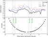 |
Fig. 1 Top panel: spectral misalignments in three regions around the Na doublet, the Hα, and the Ca II IRT line. Bottom panel: airmass value for each exposure (two of the exposures with airmass larger than 1.8 are not shown). |
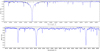 |
Fig. 2 Average Hα and Ca II IRT spectra (blue). Black lines show a telluric transmission spectrum used for the telluric correction in the Hα region. The uncorrected spectrum is shown in gray in the Hα panel. |
4 Data analysis: stellar activity
Using high-resolution transit spectra, we have two possible approaches to detect the exoplanetary sodium embedded inside the stellar spectrum: one is to integrate in narrow passbands inside the stellar absorption lines (with a reference band in the continuum) and investigate the additional contribution of the planetary atmosphere to the obscuration of the stellar light during the transit (excess light curve approach). The other is to directly obtain the exoplanetary transmission spectrum by dividing the in-transit spectra by the out-of-transit spectra (division approach). First, however, we identify possible signatures of stellar activity on the spectra. In this section, we investigate the stellar activity and then, in the following sections, we perform the transmission spectroscopy using excess light curve and division approaches.
Investigations of stellar activity
Stellar spots (e.g., Czesla et al. 2009; Oshagh et al. 2013), plage regions (e.g., Oshagh et al. 2014), and flaring activity (e.g., Klocova et al. 2017) are among the main sources of false signals in the interpretation of transmission spectra.
Small bumps or dips in the photometric transit light curves and deformations of the high-resolution spectral line shapes can be signatures of stellar variability. Investigations of spots through study of spectral line deformations are easier for very fast rotating stars (e.g., Wolter et al. 2005; Reiners 2012). In this work, as we do not have simultaneous photometric observations and the staris a slow rotator, the study of stellar spots is not possible. However we are still able to perform an in-depth study of flaring events.
Chromospheric lines such as Hα (at 6563 Å) and Ca II IRT (at 8498, 8542, 8662 Å) are indicators of stellar activity (e.g., Chmielewski 2000; Andretta et al. 2005; Cincunegui et al. 2007; Busà et al. 2007; Martínez-Arnáiz et al. 2010; Klocova et al. 2017), but also other stellar lines such as the sodium D-lines can be affected by stellar activity (e.g., Cessateur et al. 2010). Here, we estimate by how much a planetary signal in the sodium D-lines can be affected by stellar activity.
Additionally, the Hα line may indicate signatures of hydrogen escape from the upper atmosphere of hot gas planets (Cauley et al. 2016, 2017a). Due to its low mean density and a high irradiation level, WASP-17 b is expected to host a strongly evaporating atmosphere (Bourrier et al. 2015; Salz et al. 2016). Therefore, it is reasonable to search for Hα absorption features around the planetary transit.
We compute the equivalent width (EW) of the individual “transmission” spectra in the Hα and all three Ca II IRT lines following Cauley et al. (2017a). Each spectrum is divided by the total mean spectrum and then integrated over the central ±50 km s−1. The EW of the three IRT lines is then averaged. Errors are derived from the variation in adjacent ±500–1000 km s−1 bands. This slightly underestimates the error in the line cores and the impact of red-noise, and therefore we follow Czesla et al. (2017) to derive a mean error for the EW curves and scale our values accordingly.
The time evolution of the EWs is shown in Fig. 3. Both EWs evolve similarly: except for the planetary egress, WASP-17 shows a slightly increased activity level during the planetary transit compared to the out-of-transit level. This is also seen in the average in-transit transmission spectrum of the Hα and IRT regions (see Fig. A.1). At egress both EW light curves show a dip, which can be caused by stellar variability or by some absorption feature of planetary origin. However, the S/N is not sufficient to investigate this any further. The Hα EW of WASP-17 changes by about 20 mÅ over the transit duration, which is slightly stronger than that of HD 189733 (see Cauley et al. 2017a). The EW of a planetary Hα absorption feature should be smaller than the observed activity variation, which is equivalent to an absorption level 0.9% over the integration band. For the IRT we exclude 8 mÅ corresponding to 0.3% absorption. WASP-17 is among several other systems with non-detections of Hα in-transit absorption (HD 149026, HD 147506, KELT-3 b, and GJ 436 b; Jensen et al. 2012; Cauley et al. 2017b). Currently, HD 189733 (Jensen et al. 2012; Cauley et al. 2017a) and KELT-9b (Yan & Henning 2018) remain the systems with possible Hα absorption caused by the planet’s evaporating atmosphere.
In the study of Klocova et al. (2017), a moderate flare on the K-type host star HD 189733 affected the time evolution in all studied spectral lines with a similar time behavior. Khalafinejad et al. (2017) showed that the sodium lines were affected by the same flare, but on a level about a factor of 10 weaker than the Hα line. In WASP-17, the activity seen in the Hα region of 20 mÅ could affect the Na region on a 2 mÅ level, if we assume a similar scaling as in HD 189733. This is about half of the level of the observed absorption signal in the Na region (see below). However, the activity is higher during the transit and should not cause an artificial absorption signal, but rather decrease the planetary sodium signal. We do not observe a clear stellar flare and therefore do not attempt to correct the impact of stellar activity variations in the sodium region, but we do note that the observed absorption level may have been lowered by an increased in-transit activity level of the host star.
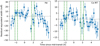 |
Fig. 3 Time evolution of the EWs of the Hα line and themean of the three Ca II IRT lines. The contact points of the transit are indicated by vertical dashed green lines. The horizontal line shows the reference value of zero. Both lines show some activity evolution over the night, but no stellar flares. |
5 Analysis and results: excess light curve approach
5.1 Extraction and modeling of the excess light curve
The extraction of the raw excess light curves in the sodium doublet region is performed by Zhou & Bayliss (2012), who use integration passbands of 0.75, 1, 1.5, and 3 Å centered on the core of each sodium line and select the interstellar sodium next to D1 (Na line with the longer wavelength) as a reference in the flux integration. For consistency with Zhou & Bayliss (2012), we use the same integration and reference bands. During the transit the radial velocity of the planet varies between − 18 and + 18 kms−1, which results in a Doppler shift of up to ± 0.35 Å. Therefore, with a passband of 0.75 Å we can still be sure that the exoplanetary feature is still located inside the integration band. Here, we use a different approach to measure the exoplanetary signal in the excess light curves. We make a combined model of differential LD and changing RV models to fit the excess light curves; the detailed explanations of these two model components are presented by Khalafinejad et al. 2017. To increase the S/N, we use the average of both sodium D-lines and do not treat the lines individually.
There are some effects that inevitably influence transit spectra or excess light curves. To accurately model the excess light curves, we take the following effects into account and consider each as a model component of the final model, which is introduced in Sect. 5.1.4.
5.1.1 Differential limb-darkening (component A)
Stellar limb-darkening depends on wavelength (e.g., Czesla et al. 2015). Therefore, dividing the flux in the integration band by the reference band is similar to dividing two light curves with two different limb-darkening coefficients, one by the other. This division therefore affects the shape of the excess light curve and needs to be corrected for, specifically in late-type stars where the effect is more prominent. We calculate the limb-darkening coefficients in each passband using the intensity profiles of the PHOENIX model (Hauschildt & Baron 1999; Husser et al. 2013) and the quadratic limb-darkening law (Kopal 1950). More details are explained by Khalafinejad et al. (2017); the results are shown in Table 2. Since the excess light curves are already averaged out between D1 and D2, we use the average of the coefficients. The S/N of our data is not enough to consider LD coefficients as fitting parameters; therefore, this model is considered to be constant and to have no fitting parameters. We note that changing this constant model component by 50% alters the final measured sodium absorption within the 1σ error bar.
Limb-darkening coefficients (u1,u2) for the average of sodium D2 and D1 integration bands (Core) and reference (Ref.) bands with the specified wavelength ranges in the table below.
5.1.2 Planetary radial velocity (component B)
The exoplanetary spectral lines move inside the stellar lines due to the Doppler shift caused by the exoplanetary orbital motion. This results in an apparent reduction of the depth of excess light curve at the mid-transit time (Albrecht 2008; Khalafinejad et al. 2017).
To investigate the exoplanetary atmospheric absorption effect in this work, the exoplanetary sodium line is considered as a Gaussian convolved inside the stellar sodium line. This Gaussian moves inside the stellar sodium line with anoffset proportional to the change of the radial velocity of the exoplanet by the orbital motion (see Eq. 8 in Khalafinejad et al. 2017). At the same time, the moving Gaussian causes the dip in the light curve and a bumpnear the mid-transit time. The fitting parameters of this component are the width (Gaussian σNa) and the depth (Gaussian ANa) of the exoplanetary Gaussian profile. Since our raw excess light curve is the average of both sodium D1 and D2, we model the effect on both stellar sodium lines and then obtain the averages of sigma and amplitude of the Gaussian feature.
5.1.3 Neglected effects
According to Triaud et al. (2010) and Bayliss et al. (2010), WASP-17 has a large spin-orbit misalignment angle (~ 150°), and the Rossiter–McLaughlin (RM) effect does not produce a symmetric RV curve. Therefore, the variations in line shape during the transit do not completely cancel out. Based on Fig. 6 in Anderson et al. (2010), the difference between the amplitude of the curve in the blue- and red-shifted parts of the star is about 100 ms−1, which causes a spectral line position to change by 0.002 Å. This value is at least one order of magnitude smaller than what we expect for the width of the exoplanetary sodium feature. We therefore ignore the RM effect in this analysis. We note that we evaluate the influence of the RM effect on measurements of the line centers in the alignment of spectra in Sect. 6.1. However, the maximum radial velocity caused by the RM effect is smaller than the precision of the alignment, therefore no evidence of influence of this effect could be detected.
In addition, as mentioned in Sect. 4, we cannot take into account the effects of possible spots and plages in this dataset. In any case, as also confirmed through our investigation of the activity-indicating lines, we do not expect pronounced activity features on this F-type star.
5.1.4 Final model
A combination of the LD and the RV models constitutes the main model, and we also consider a normalization constant (offset) as the third model component (C) and consider the model, M, as a function of time, t:
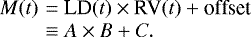 (1)
(1)
The fitting parameters in the model in Eq. 1 are the σNa, ANa, and the offset. To explore the best-fit parameters and their associated uncertainties we apply a Markov chain Monte Carlo (MCMC) analysis, using the affine invariant ensemble sampler emcee (Foreman-Mackey et al. 2013). We employ 20 walkers, with 100 chains each, where the initial positions are synthesized from a Gaussian distribution around our best estimates. All the free parameters have uniform priors imposed. For σNa and ANa, we set a lower bound of zero and upper bound of 0.3. We allow a burn-in phase of ~ 50% of the total chain length, beyond which the MCMC is converged. The posterior probability distribution is then calculated from the latter 50% of the chain (see Sect. 5.2 for the results).
5.2 Best-fit parameters and uncertainties of the excess light-curve models
The best-fit model of each excess light curve is shown in the top panels of Fig. 4 and the values of the parameters as well as their uncertainties are provided in Table 3. The posterior distributions of the fitting parameters and the correlation plots are shown in the appendix; Fig. B.1 for the 1.5 Å excess light curve. The bottom panels in Fig. 4 show residuals after subtracting the data from the model. The excess light curves have a large noise level and therefore the atmospheric absorption measurements have large uncertainties (see Table 3). As Table 3 shows, the significance of the signal is about 2σ in our narrowest integration band and the significance level reduces by the increase of the passband. At 1.5 Å there is barely any signal and the 3 Å passband results in a null outcome. At narrower passbands the contrast between the planetary and stellar flux contributions is smaller, and therefore a larger signal is expected. The measured exoplanetary signal with this approach is compared with planetary atmospheric models in Sect. 7.3.2.
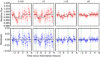 |
Fig. 4 Top panels: best-fit models plotted over the raw excess light-curves for four passbands. Bottom panels: the residuals for each passband. |
Best-fit values for the model parameters obtained from the Na D1 and Na D2 excess light curves in the three integration bands.
6 Analysis and results: division approach
6.1 Extraction of the exoplanetry spectrum through the division approach
In transmission spectroscopy we compare the spectra taken when the exoplanet is outside the transit with those taken during the transit. Only the in-transit data contain the planet’s atmospheric signatures; therefore, subtracting the out-of-transit spectrum from them can reveal the exoplanetary features within the residuals. The exoplanetary transmission spectrum is given by (Fin − Fout)∕Fout. In this simple equation, the average of all in-transit spectra is considered as Fin (master-in) and average of all of out-of transit spectra is considered as Fout (master-out). However, this method has a problem: as mentioned before, due to orbital motion, the exoplanetary RV changes and this causes shifts of the planetary sodium features relative to the stellar spectrum; the signal is therefore diluted in the process of division. To overcome this problem, after telluric corrections and alignment of spectra, we divide each individual in-transit spectrum by the master-out spectrum. Then, to line up the exoplanetary features, we shift each residual based on the corresponding calculated radial velocity of the exoplanet in each exposure. We finally co-add all residuals (similar to Wyttenbach et al. 2015, 2017) and normalize the result with the same method explained in Sect. 3. We then consider the normalized residual as the transmission spectrum (see Sect. 6.2 and Fig. 5, middle panel). By this method we correct for the RV component in the division approach as well.
It is important to note that in high-resolution transmission spectroscopy, accurate alignment of the spectra is a very important step of the analysis. In the division, slight misalignments can cause systematic dips or spikes in the residuals. The precision of the alignment depends on the S/N and on the wavelength sampling (or the resolution) of spectra. Simulating the scatter and the wavelength sampling of our spectra on a Gaussian or Voigt distribution, we obtain an uncertainty of up to 0.004 Å for the line position. This amount of mis-alignment can still be a source of variations in residuals at the location of strong lines compared tothe noise level at the continuum. Dividing two sets of out-of-transit spectra by each other is a good approach to test the alignment and the robustness of the signals in transmission spectra. Therefore, we additionally divide the average of one set of out-of-transit spectra by another: Average of exposures 1–4, taken before ingress, divided by the average of exposures 30–34, taken after egress (see Sect. 6.2 and Fig. 5, bottom panel). These two sets of out-of-transit spectra have similar airmass, and therefore a second-order correction of the tellurics may be required. In addition, in the case of this target, we can use the interstellar sodium lines as a reference for evaluation of the alignment. The interstellar lines are constant and in the division are therefore expected to result in values that are uniformly scattered around unity. Therefore, if the initial alignment does not satisfy this condition, an additional shift can be applied to improve the alignment. In each single division stage in our analysis, we manually shift each in-transit spectrum with respect to the master-out, in an attempt to minimize the variations of the residuals at the position of interstellar lines. The shifts we apply are between 0 and ± 0.004 Å in size (with the steps of 0.0005 Å) which is less than the precision of the initial alignment method. However, the final outcome with this method does not considerably alter the transmission spectrum and the residuals of the interstellar features do not reduce by the additional manual shifts. In Fig. 5, the result of a set of manual shift trials on in-transit exposures are shown in gray beneath the red profile. In contrast, in the case of division of two sets of out-transit spectra, applying an additional shift of about 0.004 Å to one of the spectra reduces the scatter of residuals. In Fig. 5 (bottom panel), the gray profile shows the initial division and the green profile shows the division after applying the manual shifts.
We also need to identify the effect that may cause a difference between the alignment of interstellar and t stellar lines. The RM effect is a possible source that affects the stellar lines but does not influence the interstellar lines. Based on the literature values of the orbital parameters (Anderson et al. 2011), we simulated a model of the RM effect in transit of WASP-17b and reduced it from the values of the spectral mis-alignment introduced in Sect. 3. The RM model is shown in Fig. 6 on top of spectral shift values. The largest difference that the RM effect can cause is up to 0.003 Å which is again below the precision of the initial alignment with our method. The removal of the RM effect from the shifts does not considerably affect the residual outcome (similar to the manual shifts in the second panel). Therefore, we continue the work while ignoring this effect.
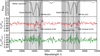 |
Fig. 5 Transmission spectrum obtained using the division approach. The black profile in the first panel is the stellar spectrum. The red profile in the second panel is the division of the in-transit by the out-of-transit spectra, corrected for the exoplanetary RV shifts. The dark gray profile beneath the red profile is the division after applying the trial manual shifts. The dark gray profile in the third panel is the division of two sets of out-of-transit spectra. The green profile is the same division shifted with respect to the other by 0.004 Å. Finally, the shaded regions represent the integration bands at 0.75, 1, 1.5, and 3 Å. |
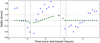 |
Fig. 6 RM model vs. spectral misalignments of sodium region. Blue crosses show the misalignment in the sodium lines region (already shown in Fig. 1). Green field circles show the calculated RM effect. Red dash-dotted line shows the alignment precision of the data (± 0.004 Å). The RM effect is below the precision of the alignment. |
6.2 Transmission spectrum of the division approach
Figure 5 summarizes the results of the division approach analysis. The master-out spectrum (or the stellar spectrum) isshown in the top panel, where the stellar and interstellar sodium lines can be clearly seen. The second panel shows the radial-velocity-corrected transmission spectrum of WASP-17b. The exoplanetary sodium absorption by D1 is visible at 5896 Å and the absorption at D2 is placed at 5890 Å. Fitting a Gaussian in each sodium feature in the transmission spectrum yields  = (0.085 ± 0.034) Å and
  = (1.3 ± 0.6)%. The error of each Gaussian fit is estimated through a MCMC procedure, where the error bar on each residual data point is equal to the standard deviation of the continuum region in the residuals scaled by the stellar flux.
Another relatively large feature we see in the residuals (middle panel) is the scatter of data at the location of interstellar sodium lines. We note that the flux values at stellar and interstellar lines are low, and therefore the S/Ns of data at the core of these lines are lower compared to the continuum. Larger scatter is therefore inevitably present in the residuals at the location of these lines (further discussed in Sect. 6.3).
Two sets of out-of-transit spectra, one divided by the other, are also shown as complementary and comparative information in the last panels of Fig. 5. Naturally, we expect no feature at the sodium line positions in this profile. We see that the scatter of the points is relatively large at stellar and interstellar sodium line positions. However, the number out-of-transit exposures that build up this profile is smaller than the profile in the second panel by about a factor of two and, on average, they are taken at larger airmass and lower S/N compared to the exposures that build up the profile in the second panel. Therefore, even in the continuum the scatter is larger compared to the second panel. Since the features in these residuals at any of the sodium lines do not exceed 3σ we consider the green profile as uniform scatter around unity.
Further discussion on evaluating the robustness of the exoplanetary absorption feature can be found in Sect. 7. Our observed transmission spectrum is then compared to a planetary atmospheric model in Sect. 7.3.1.
6.3 Residuals of the division
The residuals in Fig. 5 (middle panel) show relatively greater variation at the interstellar line positions. As discussed in Sect. 6.2, these features are related to the lower S/N at these lines. As can be seen in the top panel of the figure, the interstellar D2 line has the largest depth among all four sodium lines; the feature of the residual related to this line is also more pronounced. However, other reasons such as misalignments smaller than 0.004 Å or changes of spectral line resolutions due to Earth’s atmospheric effects can create such features. Looking at the un-binned residuals of Wyttenbach et al. (2017) for the case of WASP-49b, we see larger variations at the small interstellar sodium lines in their data as well. Compared to that work, interstellar lines in our case are stronger. In addition, MIKE is not as stable as HARPS and the resolution of our instrument is smaller by about a factor of two, meaning that the spectral alignment precision is less by about a factor of two. In any case, a complete removal of these features is not possible with this dataset and we continue the analysis assuming that features of residual spectrum at the position of the stellar sodium line are caused by the excess absorption of the exoplanetary atmosphere.
7 Discussion
7.1 Excess light curve vs. division approach
In our light curve approach we do not directly measure any light curve depth. Instead we estimate the shape of the exoplanetary sodium Gaussian profile. In the division approach we obtain the transmission spectrum in the sodium region, where the shape of the exoplanetary sodium line is directly visible.
Table 3 shows the values of widths and amplitudes of the fitted Gaussian at different passbands. The robustness of the measurements decreases with the increase of passbands, and therefore we consider themeasurement at 0.75 Å to be the best measurement. In Table 4, we compare the σNa and the ANa of exoplanetary sodium Gaussian obtained using the light curve approach, with those obtained using the division approach. Within the error bars, the values are consistent with each other.
Our measured error bars on the exoplanetary feature are relatively large. A comparison of the standard deviation of the data outside the transit with the expected signal at the sodium lines shows that the detection cannot reach confidence levels larger than 2σ and this illustrates the underestimation of the error bars in the previous analysis of the same dataset.
We note that in the division approach we do not apply any differential limb-darkening correction directly to the spectra or their residuals. However, investigation of the model components in Fig. 7 indicates that the LD model is about an order of magnitude smaller than the exoplanetary absorption effects in an F-type star; the strength of this effect is therefore already within the error bars and can be ignored in the division approach.
Sigma and amplitude of the exoplanetary Gaussian in the light curve approach vs. sigma and amplitude in the division approach.
 |
Fig. 7 Differential limb-darkening model component (dashed curve) vs. the radial velocity model component (solid curve) for the integration passband of 0.75 Å. |
7.2 Comparison to previous measurements
7.2.1 Comparison of absorption signals
In orderto be able to compare our measurements with other work, we average out the exoplanetary line flux in different passbands in both approaches. The results are shown in Table 5 and the values are compared to measurements of Zhou &Bayliss (2012) and Wood et al. (2011) obtained from high-resolution analysis. These measurements are consistent with each other within the error bars. The source of the difference between them could be in RV component correction and in the different approach in measurement of the signal. For example, Zhou & Bayliss (2012) measure the depth of the fitted light curve directly while we measure the average of the flux in the fitted exoplanetary sodium line Gaussian. By looking at Fig. 4 at 0.75 Å and roughly measuring the depth of the modeled light curve, we achieve a similar result to Zhou & Bayliss (2012).
We additionally calculate the absorption signal presented in the low-resolution transmission spectrum of WASP-17b by Sing et al. (2016) as well as the upper limit on the non-detection of sodium in the transmission spectrum obtained by Sedaghati et al. (2016). The results are also shown in Table 5. To compute the values, we measure the difference in the RP /RS value between the data point at the wavelength of sodium and the continuum level, and we also covert the radius ratios (RP /RS) to the flux ratios (Fin/Fout) to unify the units. Assuming a relation of  for the absorption as a function of passband and considering that all the exoplanetary absorption signal is coming from the line center at 0.75 Å passband, we compute the values listed in the last row of the table. If the exoplanetary sodium line wings are broader than the high-resolution passbands, then the low-resolution bin size covers the exoplanetary feature more completely. Comparison of our high-resolution expected values to the low-resolution measurements at 5 and 50 Å passbands/bin size shows that the values in low-resolution observations are larger but the results are consistent with each other within the error-bars. Influence of stellar activity can be another source of variability between the measurements of different epochs.
Estimated signal as a percentage of the stellar flux, for both light curve (LC) and division (Div.) approaches, compared to the measurments by Zhou & Bayliss (2012), Wood et al. (2011), Sing et al. (2016) and Sedaghati et al. (2016).
7.2.2 Offset between the center of the stellar and planetary sodium lines
By looking at the sodium line center in the top and middle panels of Fig. 5, we recognize an offset of ~0.15Å (7.5 kms−1) between sodium residuals and the center of the stellar sodium line. Wyttenbach et al. (2015) saw a similar shift in the Na signal of HD 189733b. We must emphasize that the alignment of the exoplanetary features before co-adding the residuals is highly dependent on the accuracy and precision of the calculated radial velocities of the exoplanet relative to its host star. In calculation of the radial velocities, changing the values of orbital parameters, that is, semi-major axis and period, even within their error bars, affects this offset. For example, considering a 2-σ upper limit on the semi-major axis calculated by Anderson et al. (2010) or a 1-σ upper limit on the semi-major axis calculated by Southworth et al. (2012), the maximum offset that we measure reaches about 6 kms−1, corresponding to about 0.12 Å.
7.3 Atmospheric physical properties
7.3.1 Comparison to atmospheric models: division approach
To model the WASP-17b high-resolution transmission spectrum and obtain a physical description of the data, we use the open-source Python Radiative Transfer in a Bayesian framework (Pyrat-Bay1, Cubillos et al., in prep.), based on the Bayesian Atmospheric Radiative Transfer package (Blecic 2016; Cubillos 2016).
Due to the wavelength normalization (Sect. 3), high-resolution transmission spectra do not constrain the planet-to-star radius ratio (as is the case for lower resolution transmission spectroscopy). For the narrow wavelength range covered by our observations, the spectra are dominated by the strong sodium doublet lines embedded into the Rayleigh absorption, which sets a continuum transmission level around the sodium lines. Thus, this data traces the differential transmission modulation of the sodium lines with respect to the Rayleigh continuum.
The Pyrat-Bay model initially computes the modulation spectrum or spectrum ratio (Brown 2001):
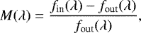 (2)
(2)
where fin(λ) and fout(λ) are the in- and out-of-transit flux spectrum, respectively. To replicate the wavelength normalization of the high-resolution data, the code calculates
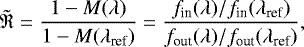 (3)
(3)
where λref is a wavelength far away from the sodium lines.
To produce the transmission spectra, the Pyrat-Bay code solves the radiative-transfer equation for a 1D atmospheric model consisting of spherically concentric layers in hydrostatic equilibrium. For the WASP-17b data, we sample the atmosphere between 100 and 10−15 bar with 200 layers. Our forward model incorporates opacities for H2 Rayleigh scattering (Lecavelier Des Etangs et al. 2008) and the sodium lines (Burrows et al. 2000). Other opacity sources like collision-induced absorption do not play a significant role at the observed wavelengths as their opacities decay exponentially as one goes toward shorter wavelengths (see, e.g., figures in Abel et al. 2011, 2012). We also discard cloud opacities based on previous transmission observations of this planet (Sing et al. 2016; Sedaghati et al. 2016).
For the retrieval, we consider the simplified case of a solar-abundance atmosphere with thermochemical-equilibrium compositions (Blecic et al. 2016). Thus, we retrieve two atmospheric parameters: the atmospheric temperature (T, as an isothermal profile) and the radius of the planet (R0) at a reference pressure p0 = 0.1 bar (necessary to solve the differential hydrostatic equation).
To explore the parameter space, Pyrat-Bay uses the differential-evolution MCMC algorithm (Cubillos et al. 2017), constrained by the high-resolution data in the three half-width at half maximum region around each sodium line. We also fit the modulation (Eq. 2) to the optical broadband transit depth 0.01524 ± 0.00027 (Sedaghati et al. 2016).
As part of our modeling approach, we solve the hydrostatic-equilibrium equation to relate the altitude and pressure profiles of the model: r = r(p). Since this is a first-order differential equation, we need a ‘boundary condition’ of the form R0 = r(p0) to obtain the particular solution of the equation. The typical procedure is to either fix R0 or p0, and then find their p0 or R0 counterpart (respectively) that fits the observations. The selection of the fixed reference point is arbitrary (we choose p0 = 0.1 bar in this article). The challenge is that transmission observations do not directly constrain the pair R0, p0, but rather allow for degenerate solutions to this problem (see, e.g., Griffith 2014). Therefore, the nature of the problem requires us to include R0 as a free parameter of the atmospheric model. We include the broadband constraint to break down one of the degeneracies of the atmospheric model, although other correlations still remain.
We adopt two configurations for the retrieval. An initial run assumes a fixed solar Na composition of 1.7 parts per million (Asplund et al. 2009), whilst allowing the temperature and reference radius to vary freely. A second run allows the sodium abundance to vary as a free parameter along with the other two parameters. All model parameters have uniform priors, and therefore the observations are the main driver of the MCMC posterior distribution.
Figure 8 shows our atmospheric model over the high-resolution transmission data (residuals) and Fig. 9 shows the best fit model and the parameter posteriors. When adopting a fixed solar sodium abundance, we retrieve an atmospheric temperature of  K, which is consistent to 1σ with the planet’s equilibrium temperature(1770 ± 35 K), and a reference radius of R0 = 1.81 ± 0.02 RJup. As expected, the retrieval with free sodium abundances has broader posterior distributions. The degeneracy of solutions leads to strongly correlated posteriors. The sodium abundance is unconstrained within our chosen exploration domain of 10−4–103 solar abundances. The retrieved temperature is
  K, while the reference radius ranges between 1.78 and 1.88 RJup.
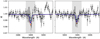 |
Fig. 8 High-resolution spectrum (black points with 1σ error bars) and best-fitting model (solid blue line) around the sodium doublet lines for the retrieval at solar Na abundance. The shaded area denotes the wavelength region used toconstrain the models. The green and red lines denote the model spectrum if R0 were 5% smaller or larger, respectively. |
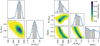 |
Fig. 9 Pairwise and marginal MCMC posterior distributions for the atmospheric retrievals with fixed (left) and free (right) Na abundance. The shaded area in the marginal posterior histograms denote the 68% highest-probability-density region of the posteriors. |
7.3.2 Comparison to atmospheric models: excess light curve approach
The model that fits the residuals at the sodium lines in division approach can be used for comparison to the excess light curve absorption signals. For this purpose, after applying the instrumental broadening, we change the sampling of the models to match the sampling of the observations and then average out the model in different passbands in the same way that we estimate the absorption signal in the observations. The result of this comparison is shown in Fig. 10. As the figure shows, the model and the observational data are coherent. Here we note that it is not practical to apply an independentatmospheric model fit to this approach, since the current model is already well within the large error bars.
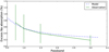 |
Fig. 10 Atmospheric model vs. observation in the excess light curve approach. The dashed blue line is the result of averaging the atmospheric model at the sodium absorption features in different passbands. The green data attached to each other by the solid line are the result of our excess light curve measurements in four different passbands. |
8 Summary and conclusions
The aim of this work is the atmospheric characterization of the inflated hot Jupiter WASP-17b using the transmission spectroscopy method in narrow wavelength bands centered on the sodium lines. We used 37 high-resolution spectra taken during a single transit of the target using the MIKE instrument on Magellan Telescopes. Our analysis consists of three main sections: (1) investigation of the stellar activity through chromospheric lines of Hα and Ca II IRT, (2) investigation of the exoplanetry sodium absorption through the excess light curves in narrow pass-bands, and (3) the same investigation but this time using an approach involving division of in-transit by out-of-transit spectra.
We detect no strong chromospheric line absorption or strong stellar variability during the observations. In the excess light curves we detect tentative signatures of exoplanetary sodium with the Gaussian width of (0.128 ± 0.078) Å and Gaussian amplitude of (1.7 ± 0.9)%. Through the division approach, the measured Gaussian width and amplitudes are (0.085 ± 0.034) Å and (1.3 ± 0.6)%, respectively. Finally, in order to extract some of the physical properties, we compare our results with the planetary atmosphericmodels. Our conclusions are as follows.
Our re-analysis of this dataset suggests underestimation of the uncertainties in the exoplanetary absorption signal measured by Zhou & Bayliss (2012). This underestimation originates in the way that the excess light curve is interpreted. In addition, we learn that, high-precision alignment (>0.004 Å) and high S/N (>100) of the spectra are crucial in achieving a robust ground-based transmission spectrum through a single transit observation. Moreover, during high-resolution transmission spectroscopy on sodium lines, simultaneous high-resolution spectral observation of the stellar activity indicators, such as Ca II H & K, Hα and Ca II IRT, reveals possible effects of stellar flaring activity on transmission spectra. Finally, through comparing our measurements with the Pyrat-Bay retrieval model, for WASP-17b we obtained an atmospheric temperature of  K, and a reference radius at 0.1bar of 1.81 ± 0.02 RJup. Overall, we have developed a framework for high-resolution transmission spectroscopy in narrow passbands inside atomic lines. This framework can be applied to higher-quality data, in order to achieve more robust exoplanetary signals at a higher confidence level.
Acknowledgements
S.K. would like to firstly thank M. Holman for providing the required funding for visiting the Center for Astrophysics (CfA), where we could establish this work. In addition, we acknowledge Deutsche Forschungsgemeinschaft (DFG), in the framework of RTG 1351 and MIN faculty of Hamburg University for providing the second part of funding of this project. C.v.E. acknowledges funding for the Stellar Astrophysics Centre, provided by The Danish National Research Foundation (Grant DNRF106). We would also like to thank B. Fuhrmeister, S. Czesla, L. Fossati, M. Lindle, M. Guedel, J. Hoeijmakers, F. Yan, and N. Espinoza for useful scientific discussions on various topics related to exoplanetray atmospheric studies. We additionally appreciate the National Collaborative Research Infrastructure Strategy of the Australian Federal Government, who supported the access to the Magellan Telescopes. We are also grateful to contributors to Numpy (van der Walt et al. 2011), SciPy (Jones et al. 2001), Matplotlib (Hunter 2007), the Python Programming Language, and the free and open-source community. Finally, we thank the anonymous referee for the useful comments which resulted in improvement of the contents of the paper.
Appendix A Transmission spectra around Hα and Ca II IRT
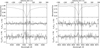 |
Fig. A.1 Leftpanel: transit spectrum of Hα. We show in the mean stellar spectrum the removed telluric absorption spectrum, the in- divided by out-of-transit spectrum and the post- divided by the pre-transit spectrum. There is an excess in the line core during the transit phase, most likely related to stellar activity. Right panel: as in the left panel but for one of the Ca II lines. |
We confirm that the source of the variations in Hα and Ca II IRT lines is stellar activity and not the exoplanetary extended atmosphere. In Fig. A.1, we show the transmission spectra in the stellar rest frame related to the Hα and one of the Ca II IRT lines. The other two Ca II IRT lines behave similarly. In the Hα region (Fig. A.1, left panel), the residuals are clean cosmic rays and telluric contamination is already removed. The strongest variation clearly occurs in the line center, and in the stellar rest frame as opposed to the planetary rest frame. We attribute this evolution to stellar activity. The IRT lines show a similar behavior (see, e.g., Fig. A.1, right panel).
Appendix B MCMC complementary figures
A sample of the MCMC posterior distribution in the excess light curve modeling is shown in Fig. B.1.
 |
Fig. B.1 Posterior distributions of the model parameters fitted in this work in the shape of histograms, along with their correlation plots, for the passband of 1.5 Å. |
References
- Abel, M., Frommhold, L., Li, X., & Hunt, K. L. C. 2011, J. Phys. Chem. A, 115, 6805 [CrossRef] [Google Scholar]
- Abel, M., Frommhold, L., Li, X., & Hunt, K. L. C. 2012, J. Chem. Phys., 136, 044319 [NASA ADS] [CrossRef] [Google Scholar]
- Albrecht, S. 2008, PhD Thesis, Leiden Observatory, Leiden University, The Netherlands [Google Scholar]
- Allart, R., Lovis, C., Pino, L., et al. 2017, A&A, 606, A144 [NASA ADS] [CrossRef] [EDP Sciences] [Google Scholar]
- Anderson, D. R., Hellier, C., Gillon, M., et al. 2010, ApJ, 709, 159 [NASA ADS] [CrossRef] [Google Scholar]
- Anderson, D. R., Smith, A. M. S., Lanotte, A. A., et al. 2011, MNRAS, 416, 2108 [NASA ADS] [CrossRef] [Google Scholar]
- Andretta, V., Busà, I., Gomez, M. T., & Terranegra, L. 2005, A&A, 430, 669 [NASA ADS] [CrossRef] [EDP Sciences] [Google Scholar]
- Asplund, M., Grevesse, N., Sauval, A. J., & Scott, P. 2009, ARA&A, 47, 481 [NASA ADS] [CrossRef] [Google Scholar]
- Bayliss, D. D. R., Winn, J. N., Mardling, R. A., & Sackett, P. D. 2010, ApJ, 722, L224 [NASA ADS] [CrossRef] [Google Scholar]
- Bento, J., Wheatley, P. J., Copperwheat, C. M., et al. 2014, MNRAS, 437, 1511 [NASA ADS] [CrossRef] [Google Scholar]
- Blecic, J. 2016, PhD Thesis [arXiv:1604.02692] [Google Scholar]
- Blecic, J., Harrington, J., & Bowman, M. O. 2016, ApJS, 225, 4 [NASA ADS] [CrossRef] [Google Scholar]
- Bourrier, V., Lecavelier des Etangs, A., & Vidal-Madjar, A. 2015, A&A, 573, A11 [NASA ADS] [CrossRef] [EDP Sciences] [Google Scholar]
- Brown, T. M. 2001, ApJ, 553, 1006 [NASA ADS] [CrossRef] [Google Scholar]
- Burrows, A., Marley, M. S., & Sharp, C. M. 2000, ApJ, 531, 438 [NASA ADS] [CrossRef] [Google Scholar]
- Busà, I., Aznar Cuadrado, R., Terranegra, L., Andretta, V., & Gomez, M. T. 2007, A&A, 466, 1089 [NASA ADS] [CrossRef] [EDP Sciences] [Google Scholar]
- Cauley, P. W., Redfield, S., Jensen, A. G., & Barman, T. 2016, AJ, 152, 20 [NASA ADS] [CrossRef] [Google Scholar]
- Cauley, P. W., Redfield, S., & Jensen, A. G. 2017a, AJ, 153, 185 [NASA ADS] [CrossRef] [Google Scholar]
- Cauley, P. W., Redfield, S., & Jensen, A. G. 2017b, AJ, 153, 81 [Google Scholar]
- Cessateur, G., Kretzschmar, M., Dudok de Wit, T., & Boumier, P. 2010, Sol. Phys., 263, 153 [NASA ADS] [CrossRef] [Google Scholar]
- Charbonneau, D., Brown, T. M., Noyes, R. W., & Gilliland, R. L. 2002, ApJ, 568, 377 [NASA ADS] [CrossRef] [Google Scholar]
- Chmielewski, Y. 2000, A&A, 353, 666 [NASA ADS] [Google Scholar]
- Cincunegui, C., Díaz, R. F., & Mauas, P. J. D. 2007, A&A, 469, 309 [NASA ADS] [CrossRef] [EDP Sciences] [Google Scholar]
- Cubillos, P. E. 2016, PhD Thesis [arXiv:1604.01320] [Google Scholar]
- Cubillos, P., Harrington, J., Loredo, T. J., et al. 2017, AJ, 153, 3 [NASA ADS] [CrossRef] [Google Scholar]
- Czesla, S., Huber, K. F., Wolter, U., Schröter, S., & Schmitt, J. H. M. M. 2009, A&A, 505, 1277 [NASA ADS] [CrossRef] [EDP Sciences] [Google Scholar]
- Czesla, S., Klocová, T., Khalafinejad, S., Wolter, U., & Schmitt, J. H. M. M. 2015, A&A, 582, A51 [NASA ADS] [CrossRef] [EDP Sciences] [Google Scholar]
- Czesla, S., Salz, M., Schneider, P. C., Mittag, M., & Schmitt, J. H. M. M. 2017, A&A, 607, A101 [NASA ADS] [CrossRef] [EDP Sciences] [Google Scholar]
- Foreman-Mackey, D., Conley, A., Meierjurgen Farr, W., et al. 2013, emcee: The MCMC Hammer, Astrophysics Source Code Library [record ascl:1303.002] [Google Scholar]
- Fortney, J. J., Shabram, M., Showman, A. P., et al. 2010, ApJ, 709, 1396 [NASA ADS] [CrossRef] [Google Scholar]
- Griffith, C. A. 2014, Phil. Trans. R. Soc. London, Ser. A, 372, 20130086 [Google Scholar]
- Hauschildt, P. H., & Baron, E. 1999, J. Comput. Appl. Math., 109, 41 [NASA ADS] [CrossRef] [Google Scholar]
- Heng, K. 2016, ApJ, 826, L16 [NASA ADS] [CrossRef] [Google Scholar]
- Hoeijmakers, H. J., de Kok, R. J., Snellen, I. A. G., et al. 2015, A&A, 575, A20 [NASA ADS] [CrossRef] [EDP Sciences] [Google Scholar]
- Høg, E., Fabricius, C., Makarov, V. V., et al. 2000, A&A, 355, L27 [Google Scholar]
- Huitson, C. M., Sing, D. K., Vidal-Madjar, A., et al. 2012, MNRAS, 422, 2477 [NASA ADS] [CrossRef] [Google Scholar]
- Hunter, J. D. 2007, Comput. Sci. Eng., 9, 90 [Google Scholar]
- Husser, T.-O., Wende-von Berg, S., Dreizler, S., et al. 2013, A&A, 553, A6 [NASA ADS] [CrossRef] [EDP Sciences] [Google Scholar]
- Jensen, A. G., Redfield, S., Endl, M., et al. 2012, ApJ, 751, 86 [NASA ADS] [CrossRef] [EDP Sciences] [Google Scholar]
- Jones, E., Oliphant, T., Peterson, P., et al. 2001, SciPy: Open Source Scientific Tools for Python, http://www.scipy.org/ [Google Scholar]
- Kempton, E. M.-R., Perna, R., & Heng, K. 2014, ApJ, 795, 24 [NASA ADS] [CrossRef] [Google Scholar]
- Khalafinejad, S., von Essen, C., Hoeijmakers, H. J., et al. 2017, A&A, 598, A131 [NASA ADS] [CrossRef] [EDP Sciences] [Google Scholar]
- Klocova, T., Czesla, S., Khalafinejad, S., Wolter, U., & Schmitt, J. H. M. M. 2017, A&A, 607, A66 [NASA ADS] [CrossRef] [EDP Sciences] [Google Scholar]
- Kopal, Z. 1950, Harvard College Observatory Circular, 454, 1 [Google Scholar]
- Lecavelier Des, A., Pont, F., Vidal-Madjar, A., & Sing, D. 2008, A&A, 481, L83 [NASA ADS] [CrossRef] [Google Scholar]
- Mandell, A. M., Haynes, K., Sinukoff, E., et al. 2013, ApJ, 779, 128 [NASA ADS] [CrossRef] [Google Scholar]
- Martínez-Arnáiz, R., Maldonado, J., Montes, D., Eiroa, C., & Montesinos, B. 2010, A&A, 520, A79 [NASA ADS] [CrossRef] [EDP Sciences] [Google Scholar]
- Moehler, S., Modigliani, A., Freudling, W., et al. 2014, A&A, 568, A9 [NASA ADS] [CrossRef] [EDP Sciences] [Google Scholar]
- Morley, C. V., Fortney, J. J., Marley, M. S., et al. 2015, ApJ, 815, 110 [NASA ADS] [CrossRef] [Google Scholar]
- Nortmann, L. 2015, PhD thesis, der Georg-August-Universität Göttingen [Google Scholar]
- Oshagh, M., Santos, N. C., Boisse, I., et al. 2013, A&A, 556, A19 [NASA ADS] [CrossRef] [EDP Sciences] [Google Scholar]
- Oshagh, M., Santos, N. C., Ehrenreich, D., et al. 2014, A&A, 568, A99 [NASA ADS] [CrossRef] [EDP Sciences] [Google Scholar]
- Pont, F., Knutson, H., Gilliland, R. L., Moutou, C., & Charbonneau, D. 2008, MNRAS, 385, 109 [NASA ADS] [CrossRef] [Google Scholar]
- Reiners, A. 2012, Liv. Rev. Solar Phys., 9, 1 [Google Scholar]
- Salz, M., Schneider, P. C., Czesla, S., & Schmitt, J. H. M. M. 2016, A&A, 585, L2 [NASA ADS] [CrossRef] [EDP Sciences] [Google Scholar]
- Seager, S., & Sasselov, D. D. 2000, ApJ, 537, 916 [NASA ADS] [CrossRef] [Google Scholar]
- Sedaghati, E., Boffin, H. M. J., Jeř abková, T., et al. 2016, A&A, 596, A47 [NASA ADS] [CrossRef] [EDP Sciences] [Google Scholar]
- Sedaghati, E., Boffin, H. M. J., MacDonald, R. J., et al. 2017, Nature, 549, 238 [NASA ADS] [CrossRef] [Google Scholar]
- Sing, D. K., Huitson, C. M., Lopez-Morales, M., et al. 2012, MNRAS, 426, 1663 [NASA ADS] [CrossRef] [Google Scholar]
- Sing, D. K., Fortney, J. J., Nikolov, N., et al. 2016, Nature, 529, 59 [NASA ADS] [CrossRef] [Google Scholar]
- Southworth, J., Hinse, T. C., Dominik, M., et al. 2012, MNRAS, 426, 1338 [NASA ADS] [CrossRef] [Google Scholar]
- Triaud, A. H. M. J., Collier Cameron, A., Queloz, D., et al. 2010, A&A, 524, A25 [NASA ADS] [CrossRef] [EDP Sciences] [Google Scholar]
- van der Walt, S., Colbert, S. C., & Varoquaux, G. 2011, Comput. Sci. Eng., 13, 22 [CrossRef] [Google Scholar]
- Vidal-Madjar, A., Sing, D. K., Lecavelier Des Etangs, A., et al. 2011, A&A, 527, A110 [Google Scholar]
- Wolter, U., Schmitt, J. H. M. M., & van Wyk F. 2005, A&A, 435, 261 [NASA ADS] [CrossRef] [EDP Sciences] [Google Scholar]
- Wood, P. L., Maxted, P. F. L., Smalley, B., & Iro, N. 2011, MNRAS, 412, 2376 [NASA ADS] [CrossRef] [Google Scholar]
- Wyttenbach, A., Ehrenreich, D., Lovis, C., Udry, S., & Pepe, F. 2015, A&A, 577, A62 [NASA ADS] [CrossRef] [EDP Sciences] [Google Scholar]
- Wyttenbach, A., Lovis, C., Ehrenreich, D., et al. 2017, A&A, 602, A36 [NASA ADS] [CrossRef] [EDP Sciences] [Google Scholar]
- Yan, F., & Henning, T. 2018, Nat. Astron., 2, 714 [NASA ADS] [CrossRef] [Google Scholar]
- Zhou, G., & Bayliss, D. D. R. 2012, MNRAS, 426, 2483 [NASA ADS] [CrossRef] [Google Scholar]
http://pcubillos.github.io/pyratbay In addition, a Reproducible Research Compendium for the Pyrat-Bay analysis is available at: https://github.com/pcubillos/KhalafinejadEtal2018_WASP17b
All Tables
Limb-darkening coefficients (u1,u2) for the average of sodium D2 and D1 integration bands (Core) and reference (Ref.) bands with the specified wavelength ranges in the table below.
Best-fit values for the model parameters obtained from the Na D1 and Na D2 excess light curves in the three integration bands.
Sigma and amplitude of the exoplanetary Gaussian in the light curve approach vs. sigma and amplitude in the division approach.
Estimated signal as a percentage of the stellar flux, for both light curve (LC) and division (Div.) approaches, compared to the measurments by Zhou & Bayliss (2012), Wood et al. (2011), Sing et al. (2016) and Sedaghati et al. (2016).
All Figures
|
Fig. 1 Top panel: spectral misalignments in three regions around the Na doublet, the Hα, and the Ca II IRT line. Bottom panel: airmass value for each exposure (two of the exposures with airmass larger than 1.8 are not shown). |
| In the text | |
|
Fig. 2 Average Hα and Ca II IRT spectra (blue). Black lines show a telluric transmission spectrum used for the telluric correction in the Hα region. The uncorrected spectrum is shown in gray in the Hα panel. |
| In the text | |
|
Fig. 3 Time evolution of the EWs of the Hα line and themean of the three Ca II IRT lines. The contact points of the transit are indicated by vertical dashed green lines. The horizontal line shows the reference value of zero. Both lines show some activity evolution over the night, but no stellar flares. |
| In the text | |
|
Fig. 4 Top panels: best-fit models plotted over the raw excess light-curves for four passbands. Bottom panels: the residuals for each passband. |
| In the text | |
|
Fig. 5 Transmission spectrum obtained using the division approach. The black profile in the first panel is the stellar spectrum. The red profile in the second panel is the division of the in-transit by the out-of-transit spectra, corrected for the exoplanetary RV shifts. The dark gray profile beneath the red profile is the division after applying the trial manual shifts. The dark gray profile in the third panel is the division of two sets of out-of-transit spectra. The green profile is the same division shifted with respect to the other by 0.004 Å. Finally, the shaded regions represent the integration bands at 0.75, 1, 1.5, and 3 Å. |
| In the text | |
|
Fig. 6 RM model vs. spectral misalignments of sodium region. Blue crosses show the misalignment in the sodium lines region (already shown in Fig. 1). Green field circles show the calculated RM effect. Red dash-dotted line shows the alignment precision of the data (± 0.004 Å). The RM effect is below the precision of the alignment. |
| In the text | |
|
Fig. 7 Differential limb-darkening model component (dashed curve) vs. the radial velocity model component (solid curve) for the integration passband of 0.75 Å. |
| In the text | |
|
Fig. 8 High-resolution spectrum (black points with 1σ error bars) and best-fitting model (solid blue line) around the sodium doublet lines for the retrieval at solar Na abundance. The shaded area denotes the wavelength region used toconstrain the models. The green and red lines denote the model spectrum if R0 were 5% smaller or larger, respectively. |
| In the text | |
|
Fig. 9 Pairwise and marginal MCMC posterior distributions for the atmospheric retrievals with fixed (left) and free (right) Na abundance. The shaded area in the marginal posterior histograms denote the 68% highest-probability-density region of the posteriors. |
| In the text | |
|
Fig. 10 Atmospheric model vs. observation in the excess light curve approach. The dashed blue line is the result of averaging the atmospheric model at the sodium absorption features in different passbands. The green data attached to each other by the solid line are the result of our excess light curve measurements in four different passbands. |
| In the text | |
|
Fig. A.1 Leftpanel: transit spectrum of Hα. We show in the mean stellar spectrum the removed telluric absorption spectrum, the in- divided by out-of-transit spectrum and the post- divided by the pre-transit spectrum. There is an excess in the line core during the transit phase, most likely related to stellar activity. Right panel: as in the left panel but for one of the Ca II lines. |
| In the text | |
|
Fig. B.1 Posterior distributions of the model parameters fitted in this work in the shape of histograms, along with their correlation plots, for the passband of 1.5 Å. |
| In the text | |
Current usage metrics show cumulative count of Article Views (full-text article views including HTML views, PDF and ePub downloads, according to the available data) and Abstracts Views on Vision4Press platform.
Data correspond to usage on the plateform after 2015. The current usage metrics is available 48-96 hours after online publication and is updated daily on week days.
Initial download of the metrics may take a while.