| Issue |
A&A
Volume 617, September 2018
|
|
|---|---|---|
| Article Number | A42 | |
| Number of page(s) | 29 | |
| Section | Interstellar and circumstellar matter | |
| DOI | https://doi.org/10.1051/0004-6361/201833196 | |
| Published online | 12 September 2018 | |
Optical and UV surface brightness of translucent dark nebulae
Dust albedo, radiation field, and fluorescence emission by H2★
1
Department of Physics, University of Helsinki,
PO Box 64,
00014
Helsinki, Finland
e-mail: mattila@cc.helsinki.fi
2
Astronomisches Institut, Ruhr-Universität Bochum, Universitätsstrasse 150,
44801
Bochum, Germany
3
Instituto de Astronomía y Ciencias Planetarias de Atacama, Universidad de Atacama,
Copayapu 485,
Copiapo, Chile
4
Korea Astronomy and Space Science Institute (KASI),
776 Daedeokdae-ro,
Yuseong-gu,
Daejeon
305-348, Korea
5
Max-Planck-Institut für Astronomie,
Königstuhl 17,
69117
Heidelberg, Germany
6
South African Astronomical Observatory,
PO Box 9 Observatory,
Cape Town, South Africa
7
Southern African Large Telescope,
PO Box 9 Observatory,
Cape Town, South Africa
8
Finnish Geospatial Research Institute FGI,
Geodeetinrinne 2,
02430
Masala, Finland
Received:
9
April
2018
Accepted:
27
May
2018
Context. Dark nebulae display a surface brightness because dust grains scatter light of the general interstellar radiation field (ISRF). High-galactic-latitudes dark nebulae are seen as bright nebulae when surrounded by transparent areas which have less scattered light from the general galactic dust layer.
Aims. Photometry of the bright dark nebulae LDN 1780, LDN 1642, and LBN 406 shall be used to derive scattering properties of dust and to investigate the presence of UV fluorescence emission by molecular hydrogen and the extended red emission (ERE).
Methods. We used multi-wavelength optical photometry and imaging at ground-based telescopes and archival imaging and spectroscopic UV data from the spaceborn GALEX and SPEAR/FIMS instruments. In the analysis we used Monte Carlo RT and both observational data and synthetic models for the ISRF in the solar neighbourhood. The line-of-sight extinctions through the clouds have been determined using near infrared excesses of background stars and the 200/250 μm far infrared emission by dust as measured using the ISO and Herschel space observatories.
Results. The optical surface brightness of the three target clouds can be explained in terms of scattered light. The dust albedo ranges from ~0.58 at 3500 Å to ~0.72 at 7500 Å. The spectral energy distribution of LDN 1780 is explained in terms of optical depth and background scattered light effects instead of the original published suggestion in terms of ERE. The far-ultraviolet surface brightness of LDN 1780 cannot be explained by scattered light only. In LDN 1780, H2 fluorescent emission in the wavelength range 1400–1700 Å has been detected and analysed.
Conclusions. Our albedo values are in good agreement with the predictions of the dust model of Weingartner and Draine and with the THEMIS CMM model for evolved core-mantle grains. The distribution of H2 fluorescent emission in LDN 1780 shows a pronounced dichotomy with a strong preference for its southern side where enhanced illumination is impinging from the Sco OB2 association and the O star ζ Oph. A good correlation is found between the H2 fluorescence and a previously mapped 21-cm excess emission. The H2 fluorescence emission in LDN 1780 has been modelled using a PDR code; the resulting values for H2 column density and the total gas density are consistent with the estimates derived from CO observations and optical extinction along the line of sight.
Key words: ISM: clouds / dust, extinction / solar neighborhood / ultraviolet: ISM
Based on observations collected at the Centro Astronómico Hispano Alemán (CAHA) at Calar Alto, operated jointly by the Max-Planck, Institut für Astronomie and the Instituto de Astrofísica de Andalucía (CSIC). Based on observations collected at the European Organisation for Astronomical Research in the Southern Hemisphere.
© ESO 2018
1 Introduction
In studies of the physics and chemical composition of the interstellar grains there has been recent renewal of interest in the observational results of the albedo a and the asymmetry parameter of the scattering function g = ⟨cosθ⟩ of the grains over the optical, UV, and near-infrared (NIR) wavelength regions, see for example Jones et al. (2016), Ysard et al. (2016), Togi et al. (2017), Lee et al. (2008), Lim et al. (2015), and Murthy (2016). Surface brightness of dark nebulae offers a good observational means for their determination. A review of earlier results has been presented by Gordon (2004).
While studying the scattered light of dark nebulae there are two other surface brightness components which have to be taken into account. They are also important and interesting on their own right.
Far UV fluorescence emission by molecular hydrogen was introduced by Duley & Williams (1980) who suggested it as an additional component to explain the high dust albedo in the far-ultraviolet (FUV) as detected by Lillie & Witt (1976). Witt et al. (1989) reported the first detection outside the solar systen. Its presence in diffuse ISM was observationally confirmed by Martin et al. (1990) and in a dark nebula by Hurwitz (1994). An all-sky survey performed with the Far Ultraviolet Imaging Spectrograph (FIMS), also known as the Spectroscopy of Plasma Evolution from Astrophysical Radiation (SPEAR; Edelstein et al. 2006a; Seon et al. 2011) has revealed its wide distribution and importance for ISM studies (Jo et al. 2017). Detailed studies have already been made of a number of individual ISM targets, including dark nebulae, and have been presented for example by Park et al. (2009), Jo et al. (2011), and Lim et al. (2015).
Extended red emission (ERE) is a photoluminence phenomenon of interstellar grains first observed in the Red Rectangle by Cohen et al. (1975), Greenstein et al. (1977), and Schmidt et al. (1980), and in reflection nebulae by Witt et al. (1984). It has been since then studied in a number of dusty interstellar environments, for a review see Witt & Vijh (2004). Its contribution is mainly between wavelengths of λ ~ 5400 and 9000 Å. Spectrophotometric observations of LDN 1780 by Mattila (1979) were interpreted by Chlewicki & Laureijs (1987), and Gordon et al. (1998), Smith & Witt (2002) and others in terms of ERE. Later on the detection of ERE was announced by Witt et al. (2008) in several high-latitude dark nebulae.
The target clouds of this study, LDN 1780 (including LDN 1778, Lynds 1962), LDN 1642 and LBN 406 (Lynds 1965), hereafter called the Draco nebula, are also well known as bright dark nebulae. For their basic properties see Table 1. Most of their diffuse light is considered to originate as scattering of the interstellar radiation field (ISRF) photons by dust grains in the clouds. While all dark nebulae exhibit the scattered light component it is not plainly visible in the cases where the nebula is projected against a bright low-galactic-latitude sky. The character of LDN 1780 surface brightness was discussed already by Struve & Zebergs (1962).
Photometric observations of LDN 1780 and their interpretation in terms of grain scattering properties were presented by Mattila (1970a,b). Hα surface brightness of LDN 1780 was suggested to be due to in situ emission by del Burgo & Cambrésy (2006). However, Mattila et al. (2007) and Witt et al. (2010) have shown that most if not all of it originates as scattered light. Detection of radio emission by spinning very small grains by Vidal et al. (2011) and of molecular hydrogen IR lines by Ingalls et al. (2011) emphasize the growing interest for LDN 1780 as a laboratory for ISM physics. For the distance of LDN 1780 we have adopted the weighted mean of the distances of the LDN 134/183/1780 group of clouds, d = 110 ± 10 pc, as determined by Schlafly et al. 2014 with optical photometry of stars from the Pan-STARRS-1 data release in the area l ~ −1° - +11°, b ~36° - 38°.
LDN 1642 has been extensively studied by optical, infared, mm- and cm- molecular and H I 21-cm lines (see e.g., Sandell et al. 1981; Lehtinen et al. 2004, and references therein). Over most of the area its extinction (AV ≲4 mag) characterizes LDN 1642 as translucent, but it has also an opaque core with AV > 15 mag. And associated with the core there are two newly formed stars (Sandell et al. 1987), a rare occurrence for such a high-latitude (b ~ −36°) cloud. Its distance is  pc, as determined with Pan-STARRS-1 data (Green et al. 2015).
The Draco nebula has been detected as an intermediate velocity H I 21-cm cloud (Goerigk et al. 1983) and has been studied also via molecular line emission and optical surface brightness (Mebold et al. 1985; Witt et al. 2008). It is at a substantial distance of ~ 800 pc (Gladders et al. 1998; Penprase & Blades 2000), making it an object belonging to the inner Galactic halo. FUV fluorescence emission of the Draco area by Park et al. (2009) and of a foreground dust filament close to the Draco main cloud by Sujatha et al. (2010) have been studied. In this paper we are mainly concerned with the brightest part, “The Head” of Draco.
Because of their different distances from the Galactic plane, LDN 1780, LDN 1642 (z ≈ 60 pc), and Draco nebula (z ≈ 400 pc) are exposed to different ISRF. Moreover, their different directions as seen from the Sun cause a different scattering geometry because of the anisotropic scattering function of dust. It is also possible that the dust scattering properties in the intermediate velocity Draco cloud differ from those in the local clouds.
Some basic properties of the sample of dark nebulae and the additional UV sources of illumination for LDN 1780.
2 Observations and archival data
We have observed LDN 1780 and Draco clouds with the same photometric equipment at the Calar Alto Observatory using the same methods and calibration. LDN 1642 was observed at ESO/La Silla using very similar methods. The homogeneity of the observational material thus enables their comparison essentially free of instrumentally based differences. In addition, we have made wide field CCD imaging with the University of Bochum VYSOS6 telescope of LDN 1780 in the BV Ri bands and of LDN 1642 in the i band. We have also used archival GALEX near and far UV data for LDN 1780 and the Draco nebula, and SPEAR/FIMS far UV data for LDN 1780.
2.1 Intermediate band surface photometry of LDN 1780 and Draco nebula
Observations of the diffuse sky brightness in the areas of L 1780 and Draco nebula were carried out using the 2.2-m and 1.23-m telescopes of the Calar Alto Observatory. Each telescope was equipped with a photoelectric photometer, with photomultiplier of type RCA 31034A-02 and an identical set of filters. The following six filters were used, with central wavelengths and, in parentheses, the half widths given in Å: Strömgren u 3500 (300) and b 4670 (200) and Omega Optical Inc. interference filters 3920 (90), 4030 (90), 5250 (250), and 5800 (120), and in addition for L1780 only, the filters 7100 (150), and 8200 (150). The response curves of the filters as well as other details of the photometersare found in Leinert et al. (1995). The observations were made in the nights 1989-05-02, 05-05, 05-06, 1990-06-21, 06-22, 06-23, and 1991-06-16.
In order to eliminate the influence of the airglow time variations we used a two-telescope technique. The 1.23-m telescope was used as a monitor and was pointed towards a fixed position (RA, Dec) in the dark nebula area during the whole measuring cycle and its integration times in each filter were synchronized with those of the 2.2-m within ~1 s. The 2.2-m telescope was used to measure several individual positions within or outside the dark cloud in an area of ~1–2 deg in size. This method was possible because the ratio of the intensities as measured at the two telescopes remained very stable during a whole night despite the temporal variations of the airglow. A simple linear interpolation between two “standard position” measurements was justified by the stability of the ratio values.
In Table 2, we give the coordinates of the observed positions in and around LDN 1780 and the Draco nebula. Also given are the 250 or 200 μm intensities as measured by the Herschel Space Observatory (Pilbratt et al. 2010) or with the ISOPHOT instrument (Lemke et al. 1996) aboard ISO (Kessler et al. 1996), as well as estimates for visual extinction. The standard position, the ON and the OFF positions are indicated for each cloud. A standard position was measured typically once or twice an hour. The 1.23-m measurements were used to calculate “interpolated standard position” values for exactly the same times when the “other positions” were measured at the 2.2-m telescope. The surface brightnesses of all the other positions, both the OFF positions outside the cloud and the ON positions within the cloud, were measured relative to the standard position. The differential surface brightness of the standard position was then determined as the excess over the mean of the OFF position values. The other ON position values were referred to the standard position value. In Table 3, we give the differences ON–OFF relative to the mean of the OFF-cloud values.
The diameter of the focal plane circular aperture for the 2.2-m photometer was 118.4 arcsec. The effective aperture solid angle was determined by mapping the response with a star placed at a grid of positions within the aperture. It was found to be 6.47 × 10⁻⁴ deg2 or 1.97 × 10⁻⁷ sterad, corresponding to an aperture correction factor of 0.76. The diameter of the aperture used at the 1.23-m telescope was 10.5 arcmin. No aperture correction factor was required because it was used as monitor only. The calibration and the determination of atmospheric extinction coefficients were done by observing in each night about ten spectrophotometric standard stars from the list of Massey et al. (1988). The extinction coefficients are given in Table 2 of Leinert et al. (1995). The surface brightness values listed in Table 3 have been corrected to outside the atmosphere using these extinction coefficients and are expressed in units of 10−9 erg cm−2 s−1 sr−1 Å−1.
Because of the small extent of regions covered (≲2 deg) and the symmetrical distribution of the OFF positions around the ON positions, no special reduction procedures were applied to correct for the (small) differential atmospheric diffuse light or zodiacal light effects. We have estimated for the 2.2-m telescope the contribution by faint stars in the measuring aperture and the instrumental straylight from off-axis stars. Measurements of the off-axis straylight were made using Vega. Then, using the Nomad star catalogue compilation (Zacharias et al. 2004, 2005) we have estimated the straylight for each ON and OFF position. Only small corrections of ≲1 × 10⁻⁹ erg cm−2 s−1 sr−1 Å−1 had to be applied to the ON–OFF differences. The values listed in Table 3 have been corrected for these effects.
Spectral energy distributions (SED) of selected positions in LDN 1780 and the Draco nebula are shown in Fig. 1. We emphasize that these SEDs represent the differential I(nebula) minus I(sky) values which have resulted directly from the observations; no correction for the diffuse galactic light has been applied here (see Sect. 3.4 for the interpretation).
Positions in Draco and LDN 1780: Calar Alto intermediate-band photometry and VYSOS surface brightness imaging.
2.2 Intermediate band surface photometry of LDN 1642
Intermediate band surface photometry of selected positions in the area of LDN 1642 has been carried out in five filters, centred at 3500 Å (u), 3840, 4160, 4700 Å (b), and 5550 Å (y), using the ESO 1-m and 50-cm telescopes at La Silla (Mattila 1990; Mattila et al. 1996). The observations were made differentially, relative to a standard position in the centre of the cloud. Subsequently, the zero level was set by fitting in Dec, RA coordinates a plane through the darkest positions well outside the bright cloud area. The 50-cm telescope monitored the airglow variations. A preliminary set of these data has already been used by Laureijs et al. (1987) to derive the dust albedo over the wavelength range 3500–5500 Å.
Calar Alto intermediate-band photometric results.
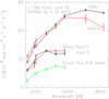 |
Fig. 1 Differential spectral energy distributions I(nebula) minus I(sky) for selected positions in LDN 1780 and the Draco nebula. The observed values are from Calar Alto photometry as described in Sect 2.1 and given in Table 3. |
2.3 Wide-field imaging of LDN 1780 and LDN 1642
We have obtained wide-field (2.7 × 2.7 deg) imaging of LDN 1780 using the University of Bochum 15 cm VYSOS6 refractor (now one of the RoBoTT twin telescopes1) located next to Cerro Armazones, northern Chile (Haas et al. 2012). It was equipped with a 4 × 4 k Alta U16M CCD-Camera of Apogee (pixel size 9 × 9 μm, corresponding to 2.37 × 2.37 arcsec). The broad band BV Ri filters had the following central wavelengths and half widths: Astrodon–Schuler BV R: B 4400 Å (1000 Å), V 5400 Å (1000 Å), R 6200 Å (1500 Å); i (Pan-STARSS) 7480 Å (1250 Å).
The observations for LDN 1780 were carried out over eight photometric nights between 2009 May 21–26 (new moon) and July 19–23 (hours with no moon). The total accumulated exposure times were 2.25 h in B and 1.25 h in V, R, and i. Imaging of LDN 1642 in the i band was carried out in 68 nights between 2009 January 16 and April 12 as part of a variable star monitoring programme. Stacking all the frames resulted in an image with 5.6 h total integration time. The frames were reduced for dark current and bias, and the flat field correction (using dome flats) was done in the standard way (Haas et al. 2012). Calibration was performed using the standard star fields LSE259, LTT6248, and SA107 (Landolt 2007). Atmospheric extinction was corrected by standard methods as explained in Haas et al. (2012).
Wide field photometry with CCD detectors has the obvious advantage over the single-channel photoelectric photometry that all pixels in the field are observed simultaneously. However, flat fielding represents a problem especially in a situation, as discussed in the present paper, where small surface brightness differences are to be discerned from a large foreground sky signal. In the single-channel approach there are no flat-fielding problems since the whole instrumental setup, that is telescope optics, instrumental effects (like internal straylight) and detector geometry and sensitivity are the same for all observed positions.
We have rescaled the VYSOS BV Ri broad band photometric maps for LDN 1780 using the results of the intermediate band results. We have determined from the VYSOS maps the differences ΔI(Pos. 1) = I(Pos. 1) − I(Pos. 33, 48), and ΔI(Pos. 10) = I(Pos. 10) − I(Pos. 33, 48) corresponding to the same ON and OFF positions used for the Calar Alto photometry. Synthetic BV Ri intensities were calculated from the intermediate-band photometry following the recipes in Leinert et al. (1995). The intensity ratios, Calar Alto/VYSOS, were 1.0, 0.97, and 1.10 for B, V, and R, respectively. For the i band a larger scaling factor of 1.46 was found. For the surface brightness determination the stars were removed from the images and the removed pixels were replaced by average background values in the surrounding area. Some residuals of the brightest stars remained but they cover only a negligible area of the maps (see the B-band image of LDN 1780 in Fig. 2 and the i-band image of LDN 1642 in Fig. 3).
2.4 GALEX FUV and NUV imaging
The Galaxy Evolution Explorer (GALEX; Martin et al. 2005) has covered a large fraction of the sky with images of 1. °25 diameter and 5′′ to 7′′ resolution in two bands, far-ultraviolet (FUV) 1350–1750 Å and near-ultraviolet (NUV) 1750–2850 Å. We have downloaded the images covering the LDN 1780 and LBN 406 areas from the GALEX archive2 where an all-sky map of the UV diffuse background is presented by Murthy (2014)3. The intensity unit of the archival images is counts s−1 cm−2 sr−1 Å −1 and the pixel size is 2′ × 2′. The conversion from photon units to cgs units is: 1 photon cm−2 s−1 sr−1 Å−1 = 1.29 × 10⁻¹¹ and 0.864 × 10⁻¹¹ erg cm−2 s−1 sr−1 Å−1 for FUV and NUV, respectively.
2.4.1 LDN 1780
GALEX archival FUV and NUV images covering an area of ~ 2.2° × 1.6° around LDN 1780 are shown in Fig. 2. In order to avoid showing the empty pixels in the Murthy (2014) data base a pixel size of 3′× 3′ has been chosen.
2.4.2 Draco nebula
GALEX archival FUV and NUV images of an area of ~ 2.5° × 2.0° covering the main part (LBN 406) of the Draco nebula is shown in Fig. 4. As for Fig. 2 the data of Murthy (2014) have been smoothed to a pixel size of 3′ ×3′. For reference, also a Herschel 250 μm and a broadband optical image (Jim Thommes 2018, priv. comm.) of the same area are shown.
2.5 SPEAR/FIMS FUV spectral imaging of LDN 1780
Archival data of SPEAR/FIMS (Edelstein et al. 2006a,b) aboard the Korean satellite STSAT−1 were utilized to study the distribution of H2 fluorescence emission in the area of LDN 1780 (see Fig. 2). The long-wavelength channel (L band; 1350–1750 Å,7. °4 × 4.′3 field of view) was used to cover a spectral region with intense H2 fluorescenceemission. The spectral and spatial resolution of the instrument are λ∕Δ λ ~ 550 and ~ 5′, respectively. We pixelated the photon data using HEALPix scheme (Górski et al. 2005) with a resolution parameter Nside = 512 corresponding to a pixel size of ~ 6.′9. After removing point sources from the image, we constructed the FUV continuum and H2 fluorescenceemission maps. They were convolved with a FWHM=0. °2. For the H2 map the continuum was first subtracted from each spectrum. The SPEAR/FIMS FUV continuum map (see Sect. 4.4 and Fig. 15) is similar to the GALEX FUV map even though, due to its lower spatial resolution, it shows a smaller peak intensity and the map details are more diffuse in comparison with GALEX. In the H2 map shown in Fig. 2 the contours of the B band surface brightness map are overplotted. As an example we show the spectrum at the H2 peak position at (RA, Dec) = (235. °5, –7. °4), SE of the LDN 1780 cloud centre. The characteristic H2 fluorescence emission features are seen in the spectrum. We will analyse the properties of the H2 emission in Sect. 4.4.
2.6 Determination of visual extinction
2.6.1 LDN 1780
Visual extinction is the natural parameter to be used in connection with modelling the scattered light. For LDN 1780 the extinction has been determined using NIR colours of background stars. In order to reach a better statistical precision than reached via the directly measured AV values we have used as proxy the 200 μm emission as mapped with ISOPHOT (Lemke et al. 1996) aboard ISO (Kessler et al. 1996).
The methods used for the determination of extinction and for the ISOPHOT 200 μm mapping have been described in detail in Ridderstad et al. (2006). In short, the optimized multi-band NICER technique of Lombardi et al. (2011) was applied to the 2MASS data. The values used for the extinction-to-colour-excess ratio were AV ∕E(J − H) = 8.86 and AV ∕E(H − KS) = 15.98; they correspond to RV = AV∕E(B − V) = 3.1 (Mathis 1990). The extinction values were averaged using a Gaussian with FWHM =3.0′. The typical total error was 0.47 mag in AV, including the variance of the intrinsic colours  and
and  and the photometric error. At the resolution of 3.0′ the value of maximumextinction is ~3.4 mag.
The extinction values as derived from 2MASS photometry are relative to a low-extinction reference field leaving, however, the extinction zero point somewhat uncertain. From three recent extinction surveys based on different methods we have found the following “absolute” extinction (AV) estimates for the VYSOS zero intensity level areas (see Table 1): AV = 0.34 mag (Schlafly & Finkbeiner 2011) (FIR emission), 0.54 mag (Schlafly et al. 2014) (Pan-STARRS), and 0.40 mag (Planck Collaboration XI 2014) (FIR and sub-mm). They are consistent with a mean value of AV = 0.43 ± 0.05 mag.
Over the mapped area of 39 × 39 arcmin2 the 200 μm intensity correlates well with AV; the relation is represented by the linear fit:
 (1)
(1)
For positions that are outside the 39 × 39 arcmin2 area we have used a Herschel SPIRE 250 μm map4 available in the Herschel archive5. A tight correlation (with an rms = 0.65 MJy sr−1) was found between I(200 μm) and I(250 μm) over the ISOPHOT map area:
 (2)
(2)
Together with Eq. (1) this then enables us to derive AV values also from I(250 μm):
 (3)
(3)
The AV values are given in Table 2.
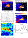 |
Fig. 2 LDN 1780 data. Upper left panel: B band VYSOS image with Calar Alto photometry positions shown as circles, the ISOPHOT 200 μm map area shown as rectangle and the two surface brightness “zero” areas as rectangles; contours are at 30.0, 23.75, 17.5, 11.25, and 5.0 ×10⁻⁹ erg cm−2 s−1 sr−1 Å−1. Upper right panel: GALEX FUV map; middle right panel: GALEX NUV map; middle left panel: map of H I 21-cm excess emission (line area), adopted from Mattila & Sandell (1979) Fig. 5; bottom left panel: SPEAR/FIMS H2 fluorescence emission map; bottom right panel: SPEAR/FIMS spectrum at RA = 15h 42m (235. °5), Dec = − 7. °4 (J2000), the brightest H2 spot in the cloud. In the GALEX images some artefacts of the 1. °25 field edges are seen as black arcs; the contours of the B band image are overplotted in the GALEX and SPEAR/FIMS for reference. Coordinates for the H I 21-cm map are RA and Dec (B1950.0); approximate J2000 coordinates have been added in red. The AB = 0. m5 extinction contour is shown as a dashed line. For the colour bars of the GALEX images and for the SPEAR/FIMS spectrum the unit is ph s−1 cm−2 sr−1 Å−1; for the colour bar of the SPEAR/FIMS H2 image the unit is ph s−1 cm−2 sr−1 (=LU, line unit). |
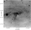 |
Fig. 3 VYSOS i band image of LDN 1642; most stars have been removed. The La Silla photometry positions that are within this image area are shown as circles. |
2.6.2 LDN 1642
We have used the NICER method (Lombardi et al. 2011) to derive extinctions from the 2MASS JHK colour excesses of stars in 6′ areas corresponding to our photometry positions in and around LDN 1642 (Mattila et al. 2017; Appendix C). However, because of the relatively low numbers of 2MASS stars at the high galactic latitude of L 1642 these extinction values had large statistical uncertainties of ca. ± 0.2−0.3 mag. The high precision achieved for I(200 μm) values (ca. ± 0.5 MJy sr−1) allows a better precision of ~±0.03 mag to be reached for AV, especially at low extinctions. Therefore, visual extinctions for our low-to-moderate extinction positions, AV ≲1mag, were determined using ISOPHOT 200 μm observations. An area of ~1.2 deg2 around L 1642 was mapped using ISOPHOT (Lehtinen et al. 2004) and, in addition, our surface photometry positions were observed also in the absolute photometry mode at 200 μm.
A fit to I(200 μm) vs. AV at I(200 μm) <30 MJy sr−1 gave the slope of 19.0 ± 2.5 MJy sr−1mag−1. The zero point of I(200 μm) was corrected for a zodiacal emission (ZE) of 0.8 ± 0.2 MJy sr−1 and a Cosmic Infared Background of 1.1 ± 0.3 MJy sr−1 (Hauser et al. 1998). The ZE at the time of our 200 μm observations (1998-03-19/20, longitude difference λ − λ⊙ =63. °7) was estimated using a 270 K black-body fit to the ZE intensities at 100, 140 and 240 μm. They were interpolated from the weekly DIRBE Sky and Zodi Atlas (DSZA)6 maps based on the Kelsall et al. (1998) interplanetary dust distribution model. The extinction values were then calculated from

We estimate their errors to be ca. ± 0.05 mag.
2.6.3 Draco nebula
The large distance and small angular size of the Draco core area make it impracticable to determine its extinction distribution with the 2MASS JHK colour excess method. The extinction mapping by Schlafly et al. (2014) using Pan-STARRS data reaches far enough (4.5 kpc) but with an insufficient resolution (14′ × 14′) for our purpose. Instead, we have used the far-infrared emission at 250 μm as a proxy for the visual extinction.
We havedetermined the AV vs. I(250 μm) relationship in two steps: (1) Miville-Deschênes et al. (2017) have mapped the Draco nebula at 250 μm using the SPIRE instrument (Griffin et al. 2010) aboard the Herschel Space Observatory (Pilbratt et al. 2010). A plot of I(250 μm), versus the optical depth at 353 GHz, derived from the Planck Surveyor all- sky survey (Planck Collaboration XI 2014), gave the relationship I(250 μm) = 6.37 105 × τ353GHz − 1.46. The intercept was removed from the I(250 μm) map to set its zero level.
(2) The second step consists of determining the connection between AV and τ353GHz. For the diffuse dust at high galactic latitudes Planck Collaboration XI (2014) have found a tight relationship between the reddening E(B − V) and τ353GHz: E(B − V) = (1.49 ± 0.039 × 10⁴) × τ353GHz which for R = AV∕E(B − V) = 3.1 corresponds to AV = 4.62 × 10⁴ τ353GHz. On the other hand, for three molecular clouds, Orion A, Orion B and Perseus, the extinction AK, derived from 2MASS JHK photometry has been correlated with τ353GHz by Lombardi et al. (2014); Zari et al. (2016) and the results are presented in Table 4 in the form

The slope γ is seen to be consistently smaller in the molecular clouds, γ = 2.20−3.51 × 10⁴, as compared to the diffuse high-latitude dust with γ = 4.62 × 10⁴. This is understood because of the higher far-IR absorption cross section of dust grains in molecular clouds vs. diffuse dust. Although the dust in the Draco nebula may be different from the “local-velocity” molecular clouds we prefer to adopt for γ the value 3.30× 10⁴, representative of the translucent parts of the Orion B and Perseus clouds, rather than the diffuse-dust value. Using this γ we end up for Draco nebula with the relationship: AV = 0.052 × I(250 μm).
This is also consistent with the relationship found in the previous Subsection for LDN 1780, The relationship for Draco “with molecular dust” is, as expected, in between the cases for “diffuse dust” and for the somewhat more opaque LDN 1780.
2.7 Optical and UV surface brightness vs. visual extinction
2.7.1 LDN 1780
The BV Ri surface brightnesses from VYSOS imaging of LDN 1780 are shown as function of visual extinction AV in Fig. 5. The surface brightnesses have been extracted for the 39′ × 39′ area covered by the ISOPHOT 200 μm map.
The zero point for the surface brightness is set in the minimum intensity areas of the VYSOS images (see Table 2 and Fig. 2). In these areas the mean extinction is AV = 0.43 mag; the zero points are indicated with black crosses in Fig. 5. In the V, R and i bands the zero level is reached within the 39′ × 39′ area of the ISOPHOT 200 μm map, but in the B band there is an offset of ~4 × 10⁻⁹ erg cm−2 s−1 sr−1 Å−1.
The B band diagram is characterized by a linear part at AV≲1.3 mag followed by a partial and then a full saturation which sets in when the extinction at the wavelength in question reaches a value of Aλ ≈ 2.5 mag. At still higher extinctions the surface brightness starts to decrease, a phenomenon that is already weakly evident at AV ≳3. The behaviour is analogous in the other bands. Because of decreasing extinction from B to i the turn-over is expected to occur, instead of at AV ~ 1.5 mag corresponding to AB ~ 2.0 mag (B), at ~ 2.0 mag (V), ~ 2.5 mag (R), and ~ 3.2 mag (i). This is also seen to be roughly the case.
The NUV and FUV surface brightnesses are plotted against the visual extinction in Fig. 8. For each raster position of the AV map, corresponding to the ISOPHOT 200 μm map positions, the mean value of the GALEX pixels within 1.8′ in l and b was taken. The zero level was set in the same area that was used also for the BV Ri bands.
The data points are shown with red symbols for the southern and black symbols for the northern half, with the division line at Dec (J2000) = − 7. °20 corresponding to the extinction maximum. Data in the Eastern “tail” area of the cloud at RA (J2000) > 15h 41m have not been included. These diagrams demonstrate quantitatively the dichotomy as seen in the UV images in Fig. 2. In the southern half the intensity is seen to increase almost linearly up to AV ~ 1 (corresponding to AFUV ≈ ANUV ≈ 2.7 mag and, after a quick turn-over, to decrease almost linearly all the way to the cloud core where AV ~ 3.5 mag, corresponding to AFUV ≈ ANUV ≈ 9.5 mag. While the INUV vs. AV curve is qualitatively similar to the IB vs. AV curve the case of the FUV band is clearly different. This cannot be explained with different extinction because it is practically the same for theNUV and FUV bands.
The northern half of the cloud (black symbols in Fig. 8) shows a very different INUV vs. AV and IFUV vs. AV relationship.All points lie below those for the southern half. Most points accumulate around a lower boundary which increases roughly linearly from the cloud’s (northern) edge to the centre. In the NUV curve there is a weak indication of a bump at AV ~ 1 mag, reminiscent of the pronounced turn-over bump on the southern half. The north–south asymmetry is clearly connected to the asymmetrical illumination of LDN 1780 in the ultaviolet. Its southern half is exposed to the UV radiation from the galactic plane and from the nearby Scorpius OB2 association.
While the BV Ri and NUV surface brightnesses can be understood in terms of scattered starlight the FUV observations require, in addition, another explanation. We will discuss in Sect. 4.4 its modelling with molecular hydrogen fluorescence emission.
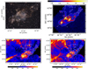 |
Fig. 4 Draco nebula images. Upper left panel: broad band optical; upper right panel: Herschel 250 μm; bottom left panel: GALEX FUV; bottom right panel: GALEX NUV. The 250 μm contours at 3, 6.6, 11, and 17 MJy sr−1 are shown and are also overplotted on the FUV and NUV images. They correspond to AV values of ~0.15, 0.36, 0.57, and 0.78 mag. The unit in the FUV and NUV colour bars is ph s−1 cm−2 sr−1 Å −1. Pixel size forFUV and NUV is 3′. At Eastern edge of the UV images the tip of the Sujatha et al. (2010) foreground filament is seen. The black area on the Western edge has no FUV and NUV data. Some artefacts of the GALEX 1. °25 field edges remain. The optical image was provided by Jim Thommes. |
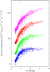 |
Fig. 5 VYSOS BV Ri surface brightness vs. visual extinction in LDN 1780. The relationships are shown from bottom to top in different colous: B (blue dots), V (green, shifted by +20 units), R (red, shifted by +40 units), and i (magenta, shifted by +60 units). The black crosses at AV = 0.43 mag indicate the zero level for each surface brightness band. |
NIR and optical extinction vs. thermal dust emission for four molecular clouds and for the high-latitude diffuse medium.
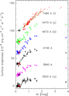 |
Fig. 6 Surface brightness vs. visual extinction in LDN 1642. The relationships are shown from bottom to top for: 3500 Å (u) (black dots), 3840 Å (magenta, shifted by +20 units), 4160 Å (black dots, +40 units), 4670 Å (b) (blue dots, +60 units), 5470 Å (green dots, +80 units), and 7478 Å (i) (red dots). The crosses at AV = 0.27 mag indicate the zero level for each surface brightness band. |
2.7.2 LDN 1642
At small optical depths with Aλ≲1 mag, the relationship is closely linear. At intermediate opacity positions with Aλ ~ 1–2 mag the scattered light has its maximum value. For still larger optical depths the scattered light intensity decreases because of extinction and multiple scattering and absorption losses (see Fig. 6).
2.7.3 Draco nebula
The maximum extinction in the Draco nebula is AV ~ 1.3 mag. In all optical bands the surface brightness vs. AV relationship appears linear over this range (see Fig. 7). The NUV and FUV surface brightness vs. AV plots are shown in Fig. 9.
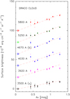 |
Fig. 7 Surface brightness vs. visual extinction in the Draco nebula. The relationships are shown from bottom to top in different colours: 3500 Å (u) (black dots), 3920 Å (magenta, shifted by +20 units), 4030 Å (blue dots, +40 units), 4670 Å (b) (blue dots, +60 units), 5250 Å (black dots, +80 units), and 5800 Å (red dots, +100 units). The crosses at AV = 0.07 mag indicate the zero level for each surface brightness band. To guide the eye approximate linear fits are shown as dashed lines. Data for positions 1 and 3 (see Table 3) deviate by more than 3σ in most colours and are not shown in this plot. |
2.8 HI 21-cm excess emission vs. optical and UV surface brightness in LDN 1780
The distribution of the HI 21-cm excess emission, adopted from Fig. 5 of Mattila & Sandell (1979) is shown in the middle panel of Fig. 2. The 21-cm excess emission is seen to be concentrated to the southern half of the cloud and its distribution is similar to the FUV distribution. Also shown in Fig. 2 is a map of the H2 fluorescence emission in the 1350–1750 Å wavelength range of SPEAR/FIMS and, as an example, the spectrum at RA = 15h 41.6m, Dec = − 7. °4 (J2000), SEof the cloud centre. The similarity of the distributions of FUV, H2 fluorescence and 21-cm excess emission is obvious and it will be further analysed and discussed in Sect. 4.4.
3 Modelling and analysis
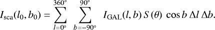
The intensity of the impinging Galactic light, as seen by a virtual observer at the cloud’s location, is a function of the galactic coordinates, IGAL = IGAL(l, b). The impinging radiation is multiply scattered by the dust grains in the cloud and the intensity of the scattered light towards the observer is given by
 (4)
(4)
For the Galactic light we have, in the optical, made use of the Pioneer10∕11 Imaging Photopolarimeter data (see Sect. 3.1.1). In the far and near UV bands data from the S2∕68 experiment aboard the TD-1 satellite are used (see Sect. 3.1.2).
S(θ) is the scattering function of the cloud; θ is the scattering angle, that is the angle between the direction l, b of the impinging radiation and the direction of the cloud, l0, b0, as seen from the observer’s viewing position. S(θ) is a function of the scattering properties of the grains (albedo a and scattering asymmetry parameter g) and the optical thickness τ of the cloud, S(θ) = S(θ, a, g, τ). We have calculated it for a set of a, g, and τ values using a Monte Carlo radiative transfer code, see Sect. 3.2.
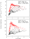 |
Fig. 8 GALEX NUV (upper panel) and FUV (lower panel) surface brightness in LDN 1780 plotted against visual extinction. The red dots are for the southern (Dec < − 7°12′), the black dots for the northern (Dec ≥−7°12′) part of the cloud (RA < 15h 41.2m for both). |
3.1 Milky Way surface brightness
For the determination of the dust albedo the intensity and distribution of the incident ISRF is equally important as that of the observed scattered light from dust. We utilize the empirical results available for the ISRF at the Sun’s location at optical and UV wavelengths. Before we can apply them to the target clouds of the present study two effects have to be taken into account: (1) the observed clouds, even if relatively nearby, are not in the Galactic plane but at a substantial z-distance of 50 to 400 pc; in the UV there may also be substantial ISRF variations caused by individual bright stars or clusters; (2) the empirical ISRF is not available for the same wavelength bands as our surface brightness observations. To account for these effects we have used a model for the star and dust distribution in the Solar Neighbourhood.
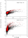 |
Fig. 9 GALEX NUV (upper panel) and FUV (lower panel) surface brightness in Draco nebula plotted against visual extinction. Red points are for the “Head” at l = 88.8−90.2 deg, b = 38.0−38.5 deg (see Fig. 4) and black points for the “Tail” part of the nebula. |
3.1.1 Optical
The Imaging Photopolarimeter instruments aboard the Pioneer 10 and 11 spacecraft got a clean measurement of the Milky Way B and R band surface brightness distributions, IGAL(l, b), duringtheirinterpanetary cruise beyond the zodiacal dust cloud at heliocentric distance of 3–5 A.U. (Weinberg et al. 1974; Toller 1981). All-sky maps have been published by Gordon et al. (1998)7. We have adopted from this web page the data files “Reformated data with all stars” which, according to the README file, “give the measurements including all the stars”, that is the stars brighter than 6. m 5 subtracted by Toller (1981) have been returned. We have divided the sky into Δ l × Δ b = 10° × 10° pixels centred at l = 5, 15, 25, …, 165, 175 deg and b = −85, − 75, …, 75, 85 deg. The Pioneermeasures were ascribed to the pixels according to their centre coordinates and the mean value for each 10° × 10° pixel was formed. The hole in the Pioneer data centred at l ≈ 225°, b ≈ 55° was filled byusing the mean values at the same galactic latitude on both sides of the hole.
The average values of the Galactic light,  , over the celestial sphere including all the stars are 114 and 152 S
 in B and R band, respectively. These values are ~12%−13% higher than the average values without the m < 6. m5 stars, 101 and 136 S
 in B and R, respectively (Toller 1981). In the cgs units used in this paper the averages over the sky including all the stars, are 136 and 151 × 10−9 erg cm−2 s−1 sr−1 Å−1 in B and R, respectively (for a compilation, see Table 5).
The Pioneer data set of Milky Way photometry is ideal because it is free of the atmospheric and interplanetary foreground components and also because it does include the Diffuse Galactic Light (DGL) which, besides the ISL, contributes substantially (~10%–35% of the ISL) to the Galactic background light (Toller 1981).
Before utilizing the Pioneer IGAL(l, b) data for our observations we need to pay attention to two modifications: (1) our observed clouds are away from the Galactic plane; (2) the VYSOS B and R filter bands differ somewhat from the Pioneer ones. Furthermore, for other filter bands, including VYSOS V and i, no corresponding, directly observed Milky Way surface brightness maps exist. They can be derived from the Pioneer B and R band maps by applying colour transformation coefficients based on Milky Way spectrum models.
To estimate these corrections we use the results of a Solar Neighbourhood Milky Way model as presented in Lehtinen & Mattila (2013). Empirical z-distributions for stars of different spectral types and dust have been used. The spectral library of Pickles (1998) was used to synthesize the ISL spectrum. The spectrum of the DGL was assumed to be a copy of the ISL spectrum. Based on the model we give in Table 6 the correction factors to be applied to the Milky Way surface brightnesses when the cloud is at a distance of z = 50 pc or z = 400 pc above the Galactic plane. Three different numbers are given: one is for the mean surface brightness over the sky (“all-sky”); the other two are for the high galactic latitudes, b >25° and b <-25°, assuming that the cloud is above the plane.
The synthetic starlight spectra for z = 50 pc andz = 400 pc are used to calculate the transformation coefficients from Pioneer B and R bands to VYSOS BV Ri, Strömgren uby and the custom-made intermediate bands, see Table 7.
Milky Way mean surface brightness  as seen from avantage point at z = 0 pc.
The Milky Way mean surface brightness as seen from a vantage point at z = 50 pc and z = 400 pc above the Galactic plane relative to the surface brightness at z = 0.
3.1.2 Ultraviolet
The UV astronomy experiment S2∕68 (Boksenberg et al. 1973) aboard the ESRO TD-1 satellite produced a star catalogue (Thompson et al. 1978) which was used by Gondhalekar et al. (1980) and Gondhalekar (1990) to derive the ISL in the four channels around 1565 Å (Δ λ= 300 Å), 1965 Å (330 Å), 2365 Å (330 Å), and 2740 Å (300 Å). Stars brighter than 1 × 10⁻¹² erg s−1 cm−2 Å−1 were individually included and for the fainter stars a small correction (≲10%) was added. The tables of Gondhalekar (1990) give the summed-up values in 10° ×10° pixels over the whole sky. The mean intensity over the sky is 88 and 36 × 10−9 erg cm−2 s−1 sr−1 Å−1 at 1565 and 2365 Å, respectively (Table 5).
The contribution of the diffuse component to the background radiation was estimated using the diffuse background results of Seon et al. (2011) based on the SPEAR/FIMS sky survey in the FUV band at 1370–1710 Å. The mean diffuse background intensities,  , for the different galactic latitude slots, separately for north and south, were read from their Fig. 9 and added to the TD-1 1565 Å ISL values. To estimate the NUV values at 2365 Å we used the scaled FUV values,
 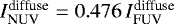 , where the coefficient has been estimated from the plot as presented in Fig. 9 of Murthy (2014). The resulting total mean Milky Way brightnesses (ISL + DGL) over the sky are 110 and 47 × 10−9 erg cm−2 s−1 sr−1 Å−1 at 1565 and 2365 Å, respectively. They are by 25% and 30% higher than the TD-1 starlight-only intensities (see Table 5). Also, Witt et al. (1997) have estimated that for an albedo a = 0.5 the scattered light increases the FUV background intensities by typically 25%.
Because of their substantial z distances the radiation field at the positions of LDN 1780, LDN 1642, and the Draco nebula differs from the one at z = 0. As in the case of the optical radiation field we have used the the results of the Solar Neighbourhood Milky Way model of Lehtinen & Mattila (2013) to estimate the corrections to be applied at the different galactic latitudes. Characteristic values are given in Table 6 for positive and negative latitudes and for the mean over the sky. Because of the narrow z-distribution of the OB stars and the stronger extinction the radiation field in the NUV and especially in the FUV is much more strongly affected by the z-distance than in the optical.
Intensity ratios of Milky Way surface brightness in different filter bands relative to B_ Pioneer and R_ Pioneer filter bands.
3.1.3 Enhanced UV radiation field for LDN 1780
LDN 1780 is located close to the directions of the Sco OB2 association and the bright O9.2 IV star ζ Oph. With the heliocentric distances of Sco OB2 (d⊙ = 144 ± 3 pc; de Zeeuw et al. 1999), ζ Oph (d⊙ = 112 ± 3 pc, Simbad; van Leeuwen 2007) and LDN 1780 (d⊙ = 110 ± 10 pc, see Sect. 1) the distances of Sco OB2 and ζ Oph from LDN 1780 are dL1780 = 54 pc and dL1780 = 28 pc, respectively. The flux which LDN 1780 receives from Sco OB2 is  7.2 times and from ζ Oph ~15.5 times as large as that received from these sources at the Sun’s position. This causes an asymmetrical and enhanced illumination of LDN 1780 especially from Sco OB2, as already suggested by Mattila & Sandell (1979) and further substantiated by Laureijs et al. (1995).
In order to estimate the FUV flux from Sco OB2 we have made use of the results of Gordon et al. (1994). Using NRL’s FUV Cameras experiment on STS-39 they imaged in two bandpasses with λeff = 1362 and 1769 Å an area of ~ 20° encompassing most of the association’s OB stars and a huge reflection nebula around them. Using IUE archives and the TD-1 catalogue (Thompson et al. 1978) they found the total stellar fluxes in these two bands to be 61.8 and 29.0 × 10⁻⁹ erg cm−2 s−1 Å−1. The contribution by the reflection nebula was found to be very substantial, amounting to 58%–92% and 68%–92% of direct starlight; the nebular contribution depended on the adopted background sky level. Assuming intermediate values of the nebular contributions of 75% and 80% and applying the distance correction factor  = 7.2 we find for the total fluxes, expressed as surface brightness contribution over the sky, the values of 62.0 and 29.3 × 10⁻⁹ erg cm−2 s−1 sr−1 Å−1.
For the GALEX FUV band we have adopted the mean of these two values: I(1540 Å) = 45.6 ×10⁻⁹ erg cm−2 s−1 sr−1 Å−1. For the GALEX NUV band we have adopted the value I(2320 Å) = 0.48 × I(1540 Å) = 21.9 ×10⁻⁹ erg cm−2 s−1 sr−1 Å−1 where the coefficient 0.48 corresponds to the intensity ratio of the GALEX NUV and FUV diffuse backgrounds as found by Murthy (2014), this may be somewhat overestimated because a bigger part of the diffuse radiation from Sco OB2 and ζ Oph than that of the general DGL may be due to H2 fluorescence. We have assumed that the foreground extinction in the direction of Sco OB2 as seen from LDN 1780 is the same as that seen from the Earth, that is the extinction of the Sco OB stars is assumed to be mainly caused by dust within the association itself.
ζ Oph has in the TD-1 catalogue (Thompson et al. 1978) the fluxes of 3.303 ± 0.011 and 1.292 ± 0.004 × 10⁻⁹ erg cm−2 s−1 sr−1 Å−1 at 1565 and 2365 Å, respectively. It has a colour excess of E(B − V) = 0.32 mag corresponding to AV = 0.90 mag, of which ≲half is thought to originate in the diffuse ISM between the star and the Sun (Liszt et al. 2009). Because the line of sight between ζ Oph and LDN 1780 is located at high altitude, z > 44 pc, we assume that the total extinction of ζ Oph as seen from LDN 1780 is AV = 0.45 and that half of the UV light removed from the star’s line of sight is returned via scattered light from the large reflection nebula surrounding it (Choi et al. 2015). With these assumptions and applying the distance correction factor of  = 15.5 we find that ζ Oph contributes by 20.8 and 9.2 ×10⁻⁹ erg cm−2 s−1 sr−1 Å−1 to the illumination of LDN 1780. This is almost half as much as the contribution by Sco OB2.
With the addition of the contributions of Sco OB2 and ζ Oph the illumination for LDN 1780 is increased to 181 and 93 ×10−9 erg cm−2 s−1 sr−1 Å−1 at 1565 and 2365 Å, respectively. These values are 1.57 and 1.65 times as large as the general Milky Way ISL+DGL surface brightness for an “observer” at z = 50 pc. For comparison, and in good agreement with this result, the direct summing-up of the radiation contributions by individual Tycho stars (for the method see Sujatha et al. 2004) results in a radiation field that is ~ 1.7 and ~ 1.4 times as large as that near the Sun in these two GALEX bands (J. Murthy, priv. comm., May 2012). As seen from L 1780 Sco OB2 and ζ Oph are seen in the directions (l, b) = (338°, -21°) and (34°, −48°), respectively. Their contributions are added to the corresponding pixels in the FUV and NUV Milky Way maps used for the L 1780 illumination. Given the distances as adopted above the scattering angle of radiation reaching us via LDN 1780 from Sco OB2 and ζ Oph is ~ 60° and ~ 70°, respectively. The direction towards Sco OB2 as projected on the sky is indicated by the arrow in the HI 21-cm map in Fig. 2.
3.2 Monte Carlo RT modelling of scattered light
We have performed a multiple scattering calculation using the Monte Carlo Method as described by Mattila (1970b). The cloud is modelled as a homogeneous sphere of optical thickness (diameter) τ. The scattering function of a single grain is assumed to have the form as introduced by Henyey & Greenstein (1941), characterized by the single scattering albedo a and asymmetry parameter g = ⟨cosθ⟩. To obtain the scattering function of the cloud, S(θ), that shall be used in Eq. (4), photons are shot into the cloud from a fixed direction. The photons leaving the cloud are classified as function of θ, the angle between the initial and the final flight direction of the photon.
It should be noticed that S(θ) refers to the scattered light from the central spot of the cloud disk, the area of the spot is 1/10th of the total disk area. In order to model the scattered light of the cloud as function of optical depth, Isca(τ), we have used spherical model clouds with different diameters τ. While this approximation does not correspond to the geometrical intuition, it still approximately takes into account the relevant optical depth and the varying amount of illumination at the off-centre cloud positions.
3.3 Effects of foreground and background dust
3.3.1 LDN 1780
It has been seen above in Sect. 2.4.1 and in Table 2 that at the OFF (=sky) positions of LDN 1780 there is an extinction ofAV ≈ 0.43 mag. From line-of-sight extinction data, available for example in Green et al. (2015), it is not possible to determine where the LDN 1780 cloud is located relative to this extended dust stratum: in front, behind or in between. The extinction in the surrounding sky area rises at 110 ± 10 pc, that is closely the same distance where the complex of high-latitude dark nebulae LDN 134, LDN 169, LDN 183, and LDN 1778/1780 is located. All these clouds are seen to be embedded in a large (~ 10°) dust envelope which is well seen in the IRAS 100 μm and Planck images as shown for example in Laureijs et al. (1995) and Planck Collaboration XI (2014). We consider it most plausible that LDN 1780 islocated about half way between the front and back side of the envelope.
Then, a layer with AV ≈ 0.215 mag would be located in front and a layer with AV ≈ 0.215 mag behind of LDN 1780. Scattered light intensity from the layer in front of LDN 1780 amounts to half, and from the layer behind of it to the other half of the total intensity at the OFF positions:
However, because of the distance uncertainty we cannot exclude the alternative that LDN 1780 is located in front of the diffuse dust envelope in which case

This case will be considered in Sect. 4.3 in addition to our standard case with equal fore- and background dust opacities.
The value of IOFF corresponding to the total line-of-sight extinction at the OFF positions is determined by fitting a straight line to the low-extinction section of the Isca vs. AV curves, as shown in Fig. 5, and extrapolating it to AV = 0. The values are given in Table 8.
We have handled the effects of the diffuse dust stratum towards L 1780 as follows: (1) The Galactic light IGAL(l, b) impinging at the boundary of the envelope is attenuated by factor ~e−τ0 where τ0 corresponds to  (OFF) = 0.215 mag. Because of scattering by the dust particles, the envelope adds a diffuse radiation field that compensates part of the attenuation. The combined effect has been tabulated for isotropic incident radiation impinging on a plane parallel layer by Whitworth (1975). The attenuation can be represented in terms of an effective optical depth, τ0 (eff). For a = 0.60, g = 0.5−0.9 we obtain from Table 1 of Whitworth τ0 (eff) = 0.55 × τ0 which results in the attenuation factors e−τ0 (eff) as given in Table 8. (2) In our model half of the scattered light of the envelope is coming from beyond LDN 1780. It is attenuated when passing through LDN 1780. Thus, we add to the model ON–OFF signal a component Δ I = Ibackground × (e−τ − 1). (3) Finally, the scattered light from the LDN 1780 cloud is attenuated by the dust layer in front of it, assumed to have an optical depth of τ0 corresponding to
  (OFF) = 0.215 mag. The attenuation factors e−τ0 are given in Table 8.
The observed surface brightness differences ON–OFF are thus modelled according to the expression:
![\begin{equation*} \mathrm{\Delta} I^{\textrm{obs}}_{\textrm{ON-OFF}}(\tau) = [I_{\textrm{sca}}(\tau) + I^{\textrm{background}}\times(\textrm{e}^{-\tau}-1)]\textrm{e}^{-\tau_0} .\end{equation*}](/articles/aa/full_html/2018/09/aa33196-18/aa33196-18-eq22.png) (5)
(5)
Parameters related to the ISRF attenuation, foreground extinction, and the off-cloud DGL models for fitting the LDN 1780 and LDN 1642 surface brightness observations.
3.3.2 LDN 1642
For LDN 1642 we treat the influence of the foreground and background dust extinction and scattered light in the same way as for LDN 1780. The assumption that the cloud is embedded in a diffuse dust stratum is based on the finding that its distance,  (Schlafly et al. 2014), coincides with that of the inner wall of the Local Bubble in its direction. This has been accurately determined by Wyman & Redfield (2013) using interstellar Na I D absorption line measurements of hipparcos stars. The OFF area extinction is AV = 0.27 mag, substantially less than that of LDN 1780. The quantities as used for the corrections, IOFF, e−τ0 (eff) and e−τ0, are given in the second part of Table 8.
3.3.3 Draco nebula
For the Draco nebula the extinction at the OFF positions is small, AV ≈ 0.065 mag (see Sect. 2.4.2 and Table 2) and it is likely caused by dust in the foreground. Thus, an additional treatment with a background dust layer is avoided. Also, the attenuation by the foreground dust layer remains small enough to be neglected in view of the other error sources.
3.4 Model fitting of the spectral energy distributions
The observed SEDs of LDN 1780 and Draco nebula as shown in Fig. 1 shall be compared with model spectra of the integrated starlight. In the scattering process the ISL spectrum, while preserving its spectral features, experiences a broad-band reddening (or bluening) that depends on the optical thickness of the cloud and the scattering properties of the grains. Because of the more qualitative aims of the SED comparison we have not made a full self-supporting RT modelling according to Eq. (4). Rather, following the the analysis of Witt et al. (2008) the scattered light spectra of the ON-cloud positions with AV ~ 1−3 mag have been approximated using the ansatz
![\begin{eqnarray*} \lefteqn{I^{\textrm{sca}}_{\lambda}(\textrm{cloud})} \nonumber \\ & {} = [C_V I^{\textrm{ISL}}_{\lambda} \textrm{e}^{-\tau_{\lambda}^{\textrm{eff}}} (1 - \textrm{e}^{-\tau_{\lambda}(\textrm{cloud})}) + I^{\textrm{sca}}_{\lambda}(\textrm{bg}) \textrm{e}^{-\tau_{\lambda}(\textrm{cloud})}] \textrm{e}^{-\tau_{\lambda}(\textrm{fg})} ,\end{eqnarray*}](/articles/aa/full_html/2018/09/aa33196-18/aa33196-18-eq24.png) (6)
(6)
where  represents the model SED for the ISL; CV is a scaling factor used to adjust the model SED intensity level at 5500 Å to the observed spectrum; τλ (cloud) is the line-of-sight optical depth through the cloud at the observed position; and τλ (fg) is the optical depth of the foreground dust layer. The term 1 −exp[−τλ(cloud)] accounts for the dependence on the finite and wavelength-dependent optical path length along the line of sight. It is a good approximation for moderate optical depths, τλ(cloud) ≲0.5.
For larger cloud thicknesses one has to account for the reddening that the impinging ISL may experience before reaching the line-of-sight column. This is the purpose of the term  where
where  can be thought to consist of two components,
  (envelope) and
  (cloud); it can encorporate also any additional reddening (or bluening), which may be required to correct for the approximative nature of the extinction correction in our ISL SED model. It is assigned as “effective” optical depth to emphasize that it is not directly given by the optical depth of the cloud and its envelope. Therefore,
  is in the first place to be understood as a fitting parameter when adjusting the ISL model SED to the observed one.
The scattered light is coming mainly from the cloud’s surface layer with τλ ≲2, facing the observer. This can be qualitatively seen from Fig. 5 where the surface brightness saturates when τλ (cloud)≳2 at the respective wavelength λ. For B band the saturation occurs at τV(cloud) ~ 1.5 whereas for the I band it happens only at τV(cloud) ~ 3.5. This situation also qualitatively demonstrates that the scattered from lines-of-sight with τV ≳1−1.5 can appear redder than the impinging ISL: while the B band intensity saturates the V to I band intensities still continue to increase.
The scattered light from the background dust layer at d > dcloud passing through the cloud is represented by the term ![$I^{\textrm{sca}}_{\lambda}(\textrm{bg})\textrm{exp}[{-\tau_{\lambda}(\textrm{cloud})}]$](/articles/aa/full_html/2018/09/aa33196-18/aa33196-18-eq31.png) . For the wavelength dependence of
. For the wavelength dependence of  , τλ (cloud), and τλ (fg) the interstellar extinction law of Cardelli et al. (1989) with RV = 3.1 was adopted.
At the sky positions, with AV≲0.5 mag, the scattered light from the background dust layer at d > dcloud can be modelled as
 (7)
(7)
where τV(bg) and τV (fg) are the optical depths of the background (d > dcloud) and of the foreground (d < dcloud) dust layer inV band. In this case the scattered light will be bluer than the impinging ISL,  ; this is demonstrated by the model SEDs for the OFF position backround light shown in the upper and middle panels of Fig. 14.
The observed surface brightness “cloud minus sky” is then given by
 (8)
(8)
The scattered light intensity of the foreground dust layer (d < dcloud) is assumed to be the same towards the cloud and the sky: it cancels out in the difference.
We have calculated the ISL spectra,  , using a synthetic model of the Solar neighbourhood as described in Sect. 3.1.1. The calculations were made for different galactic latitudes and for three locations in the Solar neighbourhood: at z = 0, 50, and 400 pc, the latter two corresponding to the locations of LDN 1780 and Draco nebula. For a single-scattering phase function of Henyey & Greenstein (1941) with g = 0.80, about 70% of light is scattered within an angle of θ <30°. Thus, the illumination for LDN 1780 and Draco nebula from the sky area behind the cloud, that is from galactic latitudes of b =10° − 70°, is heavily weighted. This is however, counterweighted by the brighter ISL in other parts of the sky. For the Draco nebula (assumed to be at z = 400 pc) the B band sky background at b ~ 36° is only ~ 17% of the mean sky brightness and ~ 18% of the corresponding value at b ~ −36° (see also Table 6).
For the purpose of comparing the observed spectra with the ISL model spectra we have adjusted in Eq. (6) the parameters CV and  in such a way that a best overall agreement was found. The V -band sky background intensity,
  (bg), has been estimated independently as described in Sects. 3.3.1 and 3.3.2 (see also Table 8). For other wavelengths
  (bg) was calculated using Eq. (7).
4 Results and discussions
4.1 Dust albedo in the optical
Model fits of scattered light data in LDN 1780 are shown in Fig. A.1 for B and R bands and in Fig. A.2for the u band. Models are shown for four different scattering parameters, g = 0, 0.50, 0.75, and 0.90, and for a range of albedos as indicated in the figures. Corresponding figures are utilized for LDN 1642 and the Draco nebula.
As can be seen from the figures the observational data enable, for each g value, a determination of the albedo with a good precision, typically ± 0.05. While at lowextinctions, AV≲1 mag, Isca is linearly proportional to albedo, the dependence is substantially steeper at intermediate and high extinction values, AV = 1.5−4 mag. This is caused by the increasing contribution of multiple scattering with increasing optical depth.
The albedo values as function of the asymmetry parameter g are shown in Fig. 10 for six different wavelength bands. Two or more filter bands are grouped together in the cases 3850/3920/4030/4160 Å, B/b, and V /y/5250/5800 Å.
In the bands between 3500 and 5500 Å all three clouds have been observed. They show different a vs. g dependences: while LDN 1642 and LDN 1780 have a moderately rising albedo from g = 0 to g = 0.90 the curve for Draco nebula is a much steeper one, ranging from a ~ 0.25 to ~0.75 for V∕y and from a ~ 0.3 to ~0.9 for the B∕b band. This behaviour is caused by the anisotropy of the impinging Galactic ISRF: if g = 0 the cloud scatters with roughly equal weight the light from all directions, while for g = 0.75−0.90 the illumination comes with higher weight from the dimmer sky area behind the cloud at high galactic latitudes, |b| >25° − 40°. With increasing z-distance from ~50–60 pc for LDN 1780 and LDN 1642 to ~400 pc for Draco the ISRF anisotropy is strongly enhanced (see Table 6). On the other hand, when a cloud is projected against the bright areas near the galactic equator its surface brightness shows an opposite trend: it decreases with increasing value of g. To qualitatively demonstrate this effect we have plotted in Fig. 10 also the UBV band results for Coalsack (l, b ≈301°, −1°) according toMattila (1970b).
If we assume that the scattering properties of dust are the same in LDN 1642, LDN 1780, and Draco nebula then the crossing area of the three loci in the a, g plane provides a determination of both parameters. For the B∕b and V∕y bands this results in the values g ~ 0.80, a ~ 0.70, and g ~ 0.80, a ~ 0.60, respectively. For the u and 3850/3920/4030/4160 Å bands somewhat smaller g-parameter values of ~ 0.60 and ~ 0.65 are indicated, resulting in albedo values of 0.50 and 0.60, respectively. If, on the other hand, g = 0.80 is adopted also for these bands, then slightly larger albedos of 0.58 and 0.63 are obtained from the LDN 1780 and LDN 1642 data. Because of the larger z-distance of Draco larger correction factors have been applied, especially for the u and 3850–4030 Å bands (see Tables 6 and 7). In view of these uncertainties the uniform value of g = 0.80 appears preferable also for these bands. We give in Table 9 and Fig. 11 the resulting albedo values when g = 0.80 is adopted.
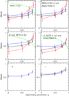 |
Fig. 10 Albedo values vs. asymmetry parameter g derived from modelling as shown in Fig. A.1. Results are shown for LDN 1780 (blue symbols), LDN 1642 (black), and Draco nebula (red). For reference also the results for the Coalsack are shown in the UBV bands (green lines) (Mattila 1970b). |
Albedo values a for asymmetry parameter value g = 0.80.
4.2 Ultraviolet dust albedo
The ultraviolet surface brightness distribution in LDN 1780 differs from that in the optical (Fig. 2). It is, especially in the FUV band, much stronger in the southern half of the nebula (Dec < −7°15′) as comparedwith positions with the same AV in the northern half. For a quantitative presentation see Fig. 8. A somewhat similar dichotomy, though much less pronounced, is observed also between the “Head” and the “Tail” parts of the Draco nebula (see Figs. 4 and 9). This behaviour can be understood for the Draco nebula (both FUV and NUV) and LDN 1780 (NUV, but not FUV as shown below) in terms of scattered light, with enhanced illumination from the hemisphere facing the galactic plane and with strong intra-cloud shadowing by the dust in UV.
We show in Fig. 12 a plot of FUV (λ = 1344−1786Å), vs. NUV (λ = 1771−2831Å) surface brightness for LDN 1780 (lower panel) and Draco nebula (upper panel). The positions in the southern part of LDN 1780 and in the “Head” of Draco are indicated with red points; for choice of areas see explanations for Figs. 8 and 9. While the NUV intensity is likely due to scattering only, the FUV band contains, potentially, also fluorescent emission bands of H2 and spectral lines of atomic species. In Draco both the “Head” (red) and the “Tail” points (black) are seen to obey the same relationship IFUV = k INUV + b. The slope indicated with the green line corresponds to the mean INUV∕IFUV ratio of 0.48 found by Murthy (2014) for the all-sky diffuse background radiation. For LDN 1780 the “shadow-side” points (black) are seen to follow this same mean INUV∕IFUV relationship. For the “bright-side”, however, the points (red) show a different slope, and relative to the mean INUV∕IFUV value there is a FUV excess of up to ~ 25 ×10−9 erg cm−2 s−1 sr−1 Å−1; or, the ratio IFUV∕INUV is up to ~3.5 times as large as that on the “shadow side”. We interpret this behaviour as evidence for H2 fluorescence plus possible atomic emission lines and will analyse it in Sect. 4.4. (For a similar argument applied to a foreground dust filament in Draco; see Sujatha et al. 2010.)
For a strongly forward throwing scattering function, g ≥ 0.7, the starlight “from behind” dominates the illumination even for high-latitude clouds in the optical bands, 3500–8000 Å. For the NUV (2320 Å) and FUV (1540 Å) bands the situation is different: here the background starlight at high latitudes, and especially when the cloud is at high altitude (z≳200 pc), becomes so weak that light from the galactic disk dominates also for g ≥ 0.7.
The NUV observations of LDN 1780 can be reasonably well understood in terms of scattered light, see Fig. B.1. At small extinctions, AV≲1.5 mag, there is a large systematic difference between the “bright side” (red) and “dark side” (black) branches of points. However, in the cloud centre, corresponding to AV ≈ 2.5−3 mag, both branches converge. It is just here that our simple Monte Carlo simulation is also expected to be valid. Reasonable albedo estimates can thus be obtained for the g values of 0, 0.50, and perhaps also for 0.75, whereas the models for g = 0.90 do not reproduce the observations for any albedo.
In the Draco nebula the NUV intensity at AV ≈ 1 mag is by a factor of ~2−3 lower than that for LDN 1780 at the same AV. The model fits reproduce well the observed intensity vs. AV behaviour and, although the observational scatter is large, enable determination of albedo values to a precision of ~ ±0.1 for all values of g from 0 to 0.9. The NUV albedo values for LDN 1780 and Draco are shown in the lower panel of Fig. 13 as function of g.
Also the FUV observations of the Draco nebula can be satisfactorily interpreted in terms of the scattered light model curves for g = 0−0.9. Although the observational scatter at faint surface brightness levels is large it still allows the determination of the albedo to a precision of ~± 0.1 or better. Also in this case most weight is put to the positions at the highest extinction range at AV ≳1 mag where our Monte Carlo modelling corresponds best to the cloud illumination geometry. The positions in the cloud “Head” (red points in Fig. B.2) are considered to better correspond to our ISRF model and they are preferred over the “Tail” points.
In the case of FUV observations of LDN 1780 we consider that the points (red) at AV ≲2 on the “bright side” are strongly affected by H2 fluorescence emission and cannot be used for albedo estimates. Thus, the observed points at AV ≳2.5 mag, where the “bright” and “shadow” branches converge, are again preferred for the albedo determination. For g = 0 and 0.5 reasonably good fits are possible and a useful estimate appears possible for g = 0.75 but not for g = 0.9. The FUV albedo values are shown in the upper panel of Fig. 13 for the three values of g.
In Fig. 11, the NUV and FUV albedo values are shown with black symbols for the g-parameter value of 0.80 which in the optical appears reasonably well justified. However, as has been pointed out above, the observations in NUV cannot be well fitted with models for g > 0.75. And the FUV observations, especially for LDN 1780, are not well-fitted for g > 0.5. Therefore, we show in Fig. 11 the FUV and NUV albedo values also for g = 0.5 (blue symbols).
The FUV “bright side” intensity peak of LDN 1780 at AV ≈ 0.9 mag cannot be satisfactorily fitted with any combination of the scattering parameters a and g (see Fig. B.1). Even the best-fitting model curves for g = 0, a ~ 0.6 leave an excess of ~ 15 ×10−9 erg cm−2 s−1 sr−1 Å−1 or ~40 % of the total signal unexplained.
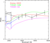 |
Fig. 11 Our derived dust albedos according to results shown in Figs. 10 and 13 and Table 9. For the black dots with error bars the g-parameter value of 0.80 has been adopted for all bands. For FUV and NUV albedos also the values for g = 0.50 are shown asblue point with error bars. For FUV (λ1540Å) and NUV (λ2320Å) the mean of LDN 1780 and Draco nebula is shown, with the Draco value at the lower and LDN 1780 value at the upper end of the error bar. Dust model albedo values are shown according to Draine (2003) (red curve), THEMIS CM (magenta), and THEMIS CMM (green) (Jones et al. 2016). |
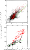 |
Fig. 12 FUVvs. NUV surface brightness in LDN 1780 (lower panel) and Draco nebula (upper panel). The southern part of LDN 1780 and the “Head” of Draco are indicated with red and the northern part of LDN 1780 and “other” parts of Draco with black dots (see Figs. 8 and 9). The mean intensity ratio for the all-sky diffuse background radiation according to Murthy (2014) is shown as the green line. |
4.2.1 Dust scattering properties: comparison with dust models
Two model concepts for grains are at present mostly being discussed and used for predicting observational phenomena of interstellar dust: (1) based on the pioneering work of Hoyle & Wickramasinghe (1969) grain models consisting of a mixture of distinct populations of bare graphite and silicate particles, each one having its own size distribution; this concept has lead to the popular MRN dust model of Mathis et al. (1977) and its modified versions presented in Draine & Lee (1984) and Weingartner & Draine (2001); (2) the so-called core–mantle grains which have graphite or silicate cores covered by ice or “organic” amorphous carbon mantles were introduced by Greenberg (1986), Duley (1987), Jones (1988), and others and are the basis of the dust modelling framework THEMIS8 (Jones et al. 2016).
Besides the wavelength dependence of extinction, the scattering properties of the grains, the albedo a and the asymmetry parameter g, are important in putting constraints on the grain models. Scattering and the determination of a and g have been studied in a variety of dusty environments; for a review see for example Gordon (2004).
In Fig. 11, we compare our observed albedo values with the predictions of three dust models: (1) the albedo values as presented in Draine (2003) for the Weingartner & Draine (2001) model (WD for short) for the “Milky Way dust” and RV = 3.1 are shown as red line; (2) albedos for two models in the THEMIS family, CM (for core–mantle, magenta line) and CMM (for core–mantle/mantle, green line) are shown according to Jones et al. (2016) and Ysard et al. (2016). In the optical, λ = 3500−7500Å, our observed albedo values (given for g = 0.8) are in good agreement both with the WD and THEMIS CMM models but lie, at most of the wavelength points, substantially above the THEMIS CM model values. In the ultraviolet (FUV and NUV) we give the albedo values for two asymmetry parameter values, g = 0.8 and g = 0.5. The values for g = 0.5 are seen to be in good agreement with both the WD and THEMIS CMM model whereas the values for g = 0.8 disagree with both.
Among the THEMIS family the CM particles represent the “basic” form, thought to prevail in the diffuse medium. Moving towards the denser phases the CMM grains have more evolved mantles of amorphous carbon and C:H compounds. The physical environment of translucent dark clouds and cloud envelopes appears to be the appropriate environment where CMM type grains prevail. The more evolved THEMIS AMM and AMMI grains, giving albedo values in close agreement with CMM grains and our observations, are thought to exist mainly in the denser core regions of molecular clouds.
Based on our results for the bands 4000 Å, B, and V the asymmetry parameter value g = 0.8 was adopted as a reasonable estimate for the whole optical wavelength band. There is also a wide agreement from studies in different environments and among most authors on a large value of g ~ (0.75−0.9) in the optical (Gordon 2004). However, in the ultraviolet bands, λ = 1350−1750Å (FUV) and λ = 1750−2850Å (NUV), our observations favoured a smaller value, g≲0.5 against g = 0.8. A trend towards a smaller g values in the ultraviolet was indicated also by our “best-fit” values g = 0.65 ± 0.1 at 4000 Å and g = 0.60 ± 0.1 at 3500 Å (see Table 9).
For the WD model the value of g (Draine 2003) increases from ~0.45 at 7500 Å to ~0.65 at 1500 Å. In the ultraviolet, λ ≤ 4000 Å this is compatible with our preference for intermediate g values but it is in contradiction with the observational values at the wavelengths, λ ≥ 4500 Å. The same problem occurs and is even more pronounced w.r.t. the THEMIS CMM grains (Ysard et al. 2016): it predicts a value of g increasing from ~0.45 at 7500 Å to ~0.8 at 1500 Å.
While it is out of the scope of the present paper to review and discuss the previous a and g determinations (see e.g., the compilation in Gordon 2004)9 we note that in their recent study Togi et al. (2017) find results closely similar to ours for the albedo in optical. Their results are based on UBV RI photometry of the translucent outer parts of the dense Taurus core Barnard 207 (LDN 1489). Their albedo values were calculated assuming that g = 0.9. In the u, 4000 Å, and B bands there is a perfect agreement with our values, but in the V, R, I bands their albedo values are by ~0.10–0.16 larger than ours. A substantial part of this could result from the different g values adopted: had we used g = 0.9 instead of g = 0.8 our albedo values would have increased by ~0.05–0.10 (see Fig. 10).
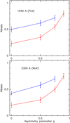 |
Fig. 13 Albedo values vs. asymmetry parameter g derived from modelling as shown in Figs. B.1 and B.2. Results are shown for LDN 1780 (blue symbols), and Draco nebula (red). |
4.3 Comparison of the SEDs of the ISL and scattered light
While the aim of Sects. 4.1 and 4.2 was to model the absolute intensity of scattered light and thereby derive the dust albedo, this section has more qualitative goals: (1) to study the connection between the spectral energy distributions (SED) of the dark nebula and that of the ISL; (2) to see if such a connection could enable to determine the location of the nebula, for example its distance; and (3) to find if the nebular surface brightness can be understood solely as scattered starlight or whether other components, such the ERE, are needed.
4.3.1 LDN 1780
For Pos. 1 and Pos. 10 in LDN 1780 the green lines in the upper and middle panels of Fig. 14 show the model spectra  (cloud) and
  (bg) for the case that the ISL spectral shape is given by the starlight at b =36°, representative of the high-latitude sky in the direction of the nebula (see Eqs. (6) and (7)). Their difference,
  , is shown as the red lines; it is to be compared with the observed differential SEDs shown as black squares with error bars. The ISL spectrum for b =36° (magenta line) is shown with normalization to the
  values at 5500 Å.
In the upper left and middle left panels of Fig. 14 the  (bg) spectra are for the case that half of the total diffuse galactic sky background light at OFF positions,
  (tot) = 15 ×10−9 erg cm−2 s−1 sr−1 Å−1, corresponding to AV = 0.43 mag, originates atdistances d > dcloud; the other half at d < dcloud has been assumed to be the same for the direction of the cloud and the sky positions and has thus canceled out in the difference (see Sect. 3.4). In the upper right and middle right panels of Fig. 14 the cloud is assumed to be in front of all widely distributed dust and, therefore, the total diffuse galactic sky backgrond light at OFF positions is ascribed to the backround component
  (bg), relevant for the ON–OFF subtraction.
In each of the four cases the model ON–OFF spectrum has been fitted to the observed SED by adjusting the parameters CV and  in Eq. (6). The best-fitting values of
  for the case of
  (bg) = 7.5 × 10⁻⁹ erg cm−2 s−1 sr−1 Å−1 were 0.70 and 0.80 for Pos. 1 and Pos. 10, respectively; for
  (bg) = 15 × cgs the
  values were somewhat smaller, 0.3 and 0.5 for Pos. 1 and Pos. 10, respectively.
From comparison of the observed with the model spectra the following conclusions can be drawn: (1) good model fits are obtained for both background choices adopted above,  (bg) = 7.5 or 15 ×10−9 erg cm−2 s−1 sr−1 Å−1. A larger
  (bg) and
  influence the differential spectrum,
  , in the same direction: making it redder. Thus, somewhat larger
  values result for our favoured case where the LDN 1780 cloud is embedded halfway within the surrounding diffuse dust envelope. We note that the
  value obtained for the higher opacity Pos. 1 (AV = 3.0 mag) is almost the same as that for Pos. 10 with the somewhat lower opacity (AV = 1.84 mag). This is as expected in the situation where the scattered light comes mostly from a τV ≲2 surface layer facing the observer (see Sect. 3.4). (2) No additional components except scattered light are needed for a good fit.
Chlewicki & Laureijs (1987) argued that the peak at ~6500 Å in the SED of LDN 1780 surface brightness (Mattila 1979) could not be explained by scattered light with the “standard” grain models, for example Mathis et al. (1977). They suggested an explanation in terms of optical fluorescence emission from grains or molecular species. In a number of papers LDN 1780 was subsequently presented as a relatively rare example of ERE occuring in a translucent dark nebula in low UV radiation density environment exhibiting a high ERE quantum yield (Gordon et al. 1998; Smith & Witt 2002; Witt & Vijh 2004).
Our multi-band photometry of LDN 1780 indicates, in agreement with Mattila (1979), the presence of a broad maximum peaking at ~6000–7000 Å. We argue, however, that our modelling in terms of scattered light only is capable of explaining this broad intensity maximum.
The fall on the long-wavelength side is jointly caused by the genuine form of the ISL’s SED with declining intensity towards the longer wavelengths and the decrease with λ of the line-of-sight optical depth through the nebula, influencing the intensity via the term 1 − exp[−τλ(cloud)].
The rise on the short-wavelength side of the peak, from ~4500 to 6000 Å, results from the combination of two effects: (1) the intensity of the diffuse galactic scattered light at the OFF (=sky) positions, from beyond the distance of LDN 1780,  (bg), is a monotonically rising function towards the shorter wavelengths; its effect is thus to make the ON–OFF signal,
  , redder; (2) reddening of the impinging ISL occurs when passing through the large-scale diffuse dust envelope in which LDN 1780 is embedded, and subsequently also within the nebula itself; these two effects are represented in Eq. (6) by the term
  .
.
For lines of sight with intermediate optical depths, τV ~ 1–3 mag, these two dust scattered light and opacity effects give rise to a broad maximum in the range ~6000–7000 Å.
While our differential SEDs of LDN 1780 can well be expla- ined in terms of reddening by dust and by the blue SED of the OFF position signal, we cannot exclude that ERE is present in LDN 1780. Because far-UV photons with energies 10.5 eV < E <13.6 eV are required for the ERE excitation (Witt & Vijh 2004; Lai et al. 2017) the ERE phenomenon is limited to low-extinction areas. In case of LDN 1780 this means that the extended diffuse dust layer covering also the OFF positions may give rise to an ERE signal as strong as that in LDN 1780, thus nulling the signal in the ON–OFF SED. And secondly, Pos. 1 and Pos. 10 represent lines of sight strongly shadowed against the far-UV photons; in the southern part of the nebula where scattered far-UV light and H2 fluorescence emission are observed (see Fig. 2), the chances for ERE detection might be better.
For optically thin lines of sight, τV≲ 0.5 mag, as was the case for the nebulae in the sample of Witt et al. (2008), a monotonically falling scattered-light SED from λ ~ 4500 to 9000 Å was found. In that case no similar confusion of the ERE signal with dust opacity effects did happen.
4.3.2 The Draco nebula
The bottom left panel of Fig. 14 shows the model fitting for the Draco nebula. In the upper part, the observed SEDs for the two highest-extinction positions, Pos. 11 (AV = 1. m27) and Pos. 13 (AV = 1. m07) are shown together with ISL spectrum models for z = 400 pc; in the lower part, the observed SEDs and the model spectra for the mean of Pos. 6 and Pos. 8 are shown. In both cases the red lines show models and model fits with ISL at b =36° as impinging radiation. In order to see how much the scattered light with larger scattering angles, θ≳30°, influences the result we show also the modelling with ISL for b = −36° (blue lines), representative of the southern hemisphere high-latitude sky, and for mean ISL over the sky (green lines). For Pos. 11/13 the best-fitting  values for b =36°, −36° and mean-over-sky ISL were 0, 1.3, and 0.6, respectively. The corresponding
  values for Pos. 6/8 were 0, 1.55, and 0.8, respectively. We note that the value of
  (bg) has been assumed to be negligible (see Sect. 3.3.3).
Good fits are obtained for both the southern-sky (b = −36°, blue curve) and mean-over-the-sky (green curve) SED models; however, the ISL spectrum for b = +36° is so red that no optimal fit was possible with  ; the fits shown in Fig. 14 for the Draco nebula are for
  = 0. This means that a very strongly forward-peaked scattering function with g ≈ 1 is not favoured.
For the location of Draco at z = 400 pc there arein the ISL spectrum for the northern and southern high-latitude sky distinct spectral differences, such as the strength of the g band, the Mg 5170 Å and the Balmer lines, and the size of the 4000 Å jump D4000. In principle, these features could be used to tell where the predominant illumination of Draco nebula is coming from. However, the coarse wavelength resolution of the present observations does not allow such a discrimination except, perhaps, in the case of D4000. A dominant contributionto Draco’s scattered light from the northern high-latitude sky would mean, however, that the dust albedo had to be ≳0.9 in the u to B bands. This is not supported by the observed intensity of the scattered light, see Sect. 4.1 and Fig. 10.
We conclude that the illumination for Draco is dominated by starlight from the galactic disk, seen from Draco’s vantage point at b < 0. In principle, the scattered light spectrum of a dark nebula could be used to determine its z-position and, thereby, also its distance from the Sun. The example with Draco demonstrates, however, that this is difficult in practice.
Historically, in the early modelling of optical cirrus clouds at high latitudes by Sandage (1976) it was suggested that their illumination is coming from “below”, that is from the galactic disk. As has been demonstrated in this paragraph it is indeed the case for a high-altitude cloud like the Draco nebula at z = 400 pc. However, most of the high-latitude clouds are, like LDN 1642 and LDN 1780, at lower altitudes, |z|≲70 pc, and, because of the strongly forward-directed scattering function of the grains, their dominant illumination in optical comes from the high-latitude sky behind them; see also Witt et al. (2008) for further discussion.
4.4 H2 fluorescence emission in LDN 1780
As has been seen above (Sect. 4.2 and Figs. 12 and B.1) there is in LDN 1780 an excess of FUV surface brightness that can not be explained in terms of scattered light. In Sect. 2.5 and Fig. 2, we have already presented SPEAR/FIMS data which demonstrate the presence of H2 fluorescence emission in the LDN 1780 FUV spectrum λ = 1450–1665 Å. To further analyse this, we present in Fig. 15 a FUV continuum map (upper left hand panel) and an H2 fluorescence emission map (upper right), both extracted from the SPEAR/FIMS data archive, processed to 0. °2 resolution. The H2 map has its peak intensity in the SE part of the cloud. The lower left hand panel of Fig. 15 shows the total and the continuum intensities plotted as function of declination from south to north. In order to increase the signal-to-noise (S/N) ratio, pixels with the same declination were merged over the right ascension range from 234. °8 to 235. °8, and the mean values were then convolved in N–S direction with FWHM=0. °2.
The difference between the total and continuum intensities can be ascribed to H2 emission; atomic lines, such as Si II* (1533 Å) and C IV (1550 Å), are negligible in the LDN 1780 spectra. The lower right hand panel of Fig. 15 shows the H2 intensity variation across LDN 1780. The peaks of the total FUV and H2 intensities are found at the same declination of − 7. °4 which is close to the southern edge of the cloud. The extinction peak (AV ~ 4 mag) is at Dec ≈ −7. °15 and the cloud edge (AV ~ 0.5 mag) at Dec ≈ −7. °45. According to Fig. 15 the H2 fluorescence emission is equally or even more strongly concentrated to the southern edge of LDN 1780 than the total FUV emission.
A substantial fraction of the total FUV intensity in LDN 1780 is due to the H2 fluorescent emission. At the intensity peak the H2 contribution to the total intensity in the FUV band is ~160 × 103 photons cm−2 s−1 sr−1 (LU; line units) or ~ 12.9 ×10⁻⁹ erg cm−2 s−1 sr−1 Å−1, which is ~2/3rds of the total intensity of ~ 19.4 ×10⁻⁹ erg cm−2 s−1 sr−1 Å−1. This is in good agreement with our previous evidence for a high level of H2 contribution to the total FUV intensity (see Figs. 12 and B.1). The total SPEAR/FIMS FUV intensity (=continuum + H2 emission) is, however, substantially lower than that for GALEX. This may be to a major part caused by the difference in the spatial resolutions of these two instruments.
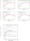 |
Fig. 14 Spectral energy distributions for Pos. 1 (upper left and upper right panels) and Pos. 10 (middle left and middle right panels)in LDN 1780, and Pos. 11 and 13 and mean of Pos. 6 and 8 in Draco nebula (bottom left panel). Observations are as in Fig. 1, model curves are according to starlight models (see text). |
4.4.1 H2 fluorescence emission from the H I–H2 transition layer in LDN 1780
When an interstellar cloud is exposed to ISRF the ground state H2 molecules absorb FUV photons in the wavelength band λ = 912−1100Å and are exited to the electronic states B and C1Πu. Some 10% of the excited H2 molecules dissociate to H atoms while the remaining 90% radiatively de-excite to vibrationally excited states of the ground electronic state X
 . These bound–bound electronic transitions give rise to H2 fluorescence emission in the Werner and Lyman bands (see e.g., Duley & Williams 1980).
H2 molecules are continuously being formed on and released from grain surfaces. Extinction and absorption of photons by dust grains and H2 molecules screen the inner parts of the cloud against UV radiation. Thus, a transition zone consisting of a mixture of H atoms and H2 molecules is formed and upheld in the cloud surface layer. In LDN 1780 such a photodissociation region (PDR) is manifested by the presence of H2 fluorescence emission and H I 21-cm excess emission in a zone at the southern edge of the cloud. As has been described in Sect. 3.1.3 above, there is an enhanced, asymmetrical FUV radiation field impinging on the cloud preferentially from the southern side.
HI-to-H2 transition zones are an important ingredient in ISM physics. With LDN 1780 we have a good opportunity to study a simple, almost spherically symmetric cloud immersed in a well-known radiation field. As can be seen from Fig. 2 the distributions of the FUV and H2 fluorescence emissions in LDN 1780 are qualitatively similar to that of the H I 21-cm excess emission. All these distributions show a bright zone along the southern edge of the nebula. Less distinctly, also the NUV intensity distribution has the same north–south dichotomy. Therefore, part of the FUV asymmetry is likely caused by the stronger illumination from the southern hemisphere, leading to stronger scattered light on that side. A substantial part of the FUV emission is, however, due to H2 fluorescence.
Duley & Williams (1980) first pointed out the possibility of detecting diffuse ultraviolet fluorescence emission from interstellar H2 and showed that its intensity in the wavelength window λ = 1400−1700Å is comparable to that of the scattered light. Following their notification the equilibrium condition for H2 formation/destruction is
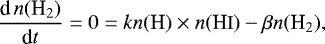 (9)
(9)
where n(HI), n(H2) and n(H) = n(HI) + 2n(H2) are the atomic, molecular and total hydrogen nucleii number densities, β is the H2 destruction rate and k the rate constant for H2 formation = 3 × 10⁻¹⁷ cm−3 s−1.
In equilibrium the H2 fluorescence volume emissivity is proportional to the number of H2 destructions
 (10)
(10)
where ⟨hν⟩ is the average photon energy. This expression refers to the fluorescence continuum emission which results from H2 dissociations, that is transitions to the vibrational continuum (v ′′ > 14) of the X electronic state. To take the transitions to the bound vibrational states (v ′′ ≤ 14) approximately into account Duley & Williams (1980) multiplied this expression by 2.
We assume that the total density n(H) can be considered to be constant in the transition layer and that the layer can be considered to be optically thin. Then, integrating J(fluorescence) along the line of sight through the nebula, one finds that the intensity of the fluorescence emission is proportional to the HI column density, I(fluorescence) ∝ N(HI). This result from the general analysis of Duley & Williams (1980) has been confirmed also by the detailed model calculations of Neufeld & Spaans (1996; see their Figs. 1 and 2).
We show in the upper and lower panel of Fig. 16 the GALEX NUV and FUV intensities in LDN 1780 as function of HI 21-cm excess line areas, W(HI), adopted from Fig. 5 of Mattila & Sandell (1979). The HI column density in LDN 1780 is directly proportional to W(HI), see Mattila & Sandell (1979). For each W(HI) value, representing the signal within 9′ FWHM beam, we have averaged the GALEX values within 6′ from the centre. The remarkably good correlation of I(FUV) vs. W(HI) especially at the larger FUV intensities, I(FUV)≳10 ×10−9 erg cm−2 s−1 sr−1 Å−1, where the fluorescence emission dominates, can be undestood as observational evidence of the linear relationship I(fluorescence) ∝ N(HI) resulting from the analysis by Duley & Williams (1980).
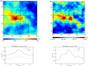 |
Fig. 15 FUV continuum and H2 fluorescence emission in LDN 1780; upper left panel: SPEAR/FIMS FUV continuum map with B band surface brightnes contours overlayed; upper right panel: the SPEAR/FIMS H2 fluorescence emission map + B band contours; lower left panel: total (red line) and continuum (blue dashed line) intensities shown as function of the declination along the path from south to north; lower right panel: H2 intensity(red line) and its statistical error (blue dashed line) along the same path across LDN 1780. The intensity unit for the total and continuum is photons cm−2 s−1 sr−1 Å−1 (CU; continuum unit) and for the line emission photons cm−2 s−1 sr−1 (LU; line unit). |
4.4.2 Modelling of the H2 fluorescence spectrum
We have modelled the H2 fluorescence emission spectrum in the FUV peak-intensity region using the CLOUD code developed for photodissociation regions assuming plane-parallel geometry (van Dishoeck & Black 1986; Black & van Dishoeck 1987; see also Lee et al. 2006, 2007, 2008; Jo et al. 2017). The following three input parameters were adopted and kept fixed during the fitting: (1) cloud temperature T = 100 K; (2) the sticking probability and formation efficiency of H2 on dust grains; we adopted yF = 1 as a typical value; (3) the strength of incident FUV radiation in the band λ = 912−1100Å, IUV, in units of the average UV radiation field of Draine (1978); we adopted the value IUV = 1.7. It is based, on one side, on the direct addition of the radiation of individual stars in the TD-1 and hipparcos star catalogues (Thompson et al. 1978; Perryman et al. 1997; see Jo et al. 2017 for details) and on the other side on the estimates as presented in Sects. 3.1.2 and 3.1.3 above. A further parameter which was allowed to vary during the fitting process was (4) the total hydrogen density; its initial value was n(H) = 1000 cm−3 based on N(H) ≈ 1 × 1021 cm−2, (corresponding to AV ≈ 0. m5) and an estimated line-of-sight cloud extent of 0.4 pc at the FUV peak position. We generated models with a range of log N(H2) values from 19.0 to 23.0 with 0.1 steps.
Before fitting the models we corrected the observed spectrum for the extinction in front of the cloud, AV = 0. m215 (see Table 8); this corresponds to an optical depth of τλ = 0.5 at λ= 1550Å. We show in the left panel of Fig. 17 the extinction-corrected spectrum (black histogram) at the FUV peak position (Dec = −7. °4, RA = 234. °8–235. °8) with the best-fit model spectrum superposed (red solid line). The best-fit model corresponds to the value log N(H2) = 20.89 with reduced χ2 = 0.976 and 1σ confidence range of 19.9–22.1, or N(H2) = 7.8 × 1020 cm−2 with 1σ confidence range of (0.8–130) × 1020 cm−2. The 1σ confidence range is wide because of the low S/N of the observed spectrum and, as seen from the left panel of Fig. 17, there are substantial deviations between the fitted and the observed spectrum. The total hydrogen column density corresponding to the best-fit N(H2) value is N(H) = 2N(H2) + N(H I) = 16.2 × 1020 cm−2, the corresponding volume density is n(H) = 1.4 × 103 cm−3. The atomic hydrogen column density is N(H I) = 0.53 × 1020 cm−2 which corresponds to an H I fractional abundance of N(H I)/2N(H2) = 0.033.
The best-fit N(H2) of the model agrees well with the observational value N(H2)=  cm−2 as estimated from the
  CO) map of Toth et al. (1995) using the factor X = N(H2)/
 CO) = 2 × 1020 cm−2 (K km s−1)−1 (Pineda et al. 2008). The derived total volume density of n(H) = 1.4 × 103 cm−3 agrees well with its initially adopted value of 1 × 103 cm−3 which was based on the line-of-sight extinction.
The strength of the incident UV radiation, IUV, is a central parameter determining the intensity of the H2 fluorescence emission I(H2). Observationally, I(H2) is seen to decrease towards the cloud centre in accord with the FUV continuum intensity (see Fig. 15). We show in the right-hand panel of Fig. 17 the calculated H2 spectra for the values IUV = 0.5, 1.0, 1.5, 1.7, 2.0, 2.5, and 3.0. All the other parameters were the same as in the best-fit model with IUV = 1.7 described above.The fluorescence emission is seen to be roughly proportional to IUV. Qualitatively, the observed decrease of I(H2) from edge towards the centre of LDN 1780 can be understood as a consequence of decreasing IUV. A quantitative analysis of the attenuation of the radiation field would, however, require a full three dimensional (3D) modelling of the radiative transfer including dust extinction and H2 self-shielding.
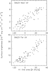 |
Fig. 16 Upper panel: GALEX NUV; lower panel: FUV intensity in LDN 1780 as a function of HI 21-cm excess line area, adopted from Fig. 5 of Mattila & Sandell (1979). |
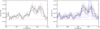 |
Fig. 17 Left panel: extinction-corrected spectrum at the FUV peak region (black histogram) and the best-fit model spectrum forIUV = 1.7 (red line). Red dashed line indicates continuum level; (right panel) as in the left-hand panel but with models for IUV = 0.5, 1.0, 1.5, 1.7 (red line), 2.0, 2.5, and 3.0. |
4.4.3 H2 fluorescence emission near LDN 1642 and Draco nebula
The TaurusMolecular Cloud (TMC) was the first dark nebula where, H2 fluorescence emission was detected (Martin et al. 1990; Hurwitz 1994). Lee et al. (2006) have analysed a dense core in Taurus as function of optical depth through the core. Their result was similar with our case with LDN 1780: a strong H2 fluorescenceemission signal was detected in the halo of the cloud with AV ≲1. m5 mag, but only a weak one or none in the core. Also the continuum FUV intensity showed a decreasing level as function of AV, again similarly with our results for LDN 1780 (see Fig. 8).
FUV continuum and H2 fluorescence emission maps with SPEAR/FIMS of the Draco nebula area have been presented by Park et al. (2009). They show a small (~ 0. °5) H2 fluorescence emission spot, centred at (l, b) = (89. °5, 38. °3), displaced by ~0. °2 from Draco’s “Head” towards the Galactic plane and partly overlapping with it. Its contribution is, however, not seen in the GALEX total FUV signal (Fig. 4), nor is there an enhancement in the SPEAR/FIMS FUV continuum map.
The Orion–Eridanus superbubble region, including LDN 1642, has been studied by Ryu et al. (2008) and Jo et al. (2011) using SPEAR/FIMS, both with regard to the dust-scattered continuum and the gaseous spectral features. The H2 fluorescent map of Jo et al. (2011) shows an enhanced intensity region ~5 deg in size, centred at R.A. ≈ 70 deg, Dec. ≈−13 deg (J2000), extending from LDN 1642 towards the Galactic plane. Interestingly, there is a large (≳5°) plume-like tail associated with LDN 1642 which is seen in the IRAS and Planck dust maps (de Oliveira-Costa et al. 2002; Malinen et al. 2014) as well as in the HI 21-cm emission (Liljestrom & Mattila 1988); it coincides relatively well with the H2 emission area both in size and location. The situation is similar as in the Draco nebula, especially if one considers that the angular size difference is partly caused by the different distances, ~800 pc for Draco vs. 124 pc for LDN 1642. The morphology of H2 emission in LDN 1642 and Draco differs, however, from that in LDN 1780: separate, possibly physically associated batches in LDN 1642 and Draco vs. a surface layer in LDN 1780.
5 Conclusions
We have presented optical surface photometry of selected positions in three translucent high-latitude dark nebulae, LDN 1780, LBN 406 (Draco nebula) and LDN 1642. Intermediate-band photometry of LDN 1780 and LBN 406 with the 2.2-m telescope at Calar Alto and of LDN 1642 with the 1-m telescope at La Silla covered the wavelength range 3500–5500/5800 Å and for LDN 1780 up to 8200 Å. Wide-field imaging of LDN 1780 in the B, V, R, i bands and of LDN 1642 in the i band were carried out using University of Bochum, 15-cm VYSOS6 refractor near Cerro Armazones, Chile. Archival data of the spaceborne instruments GALEX and SPEAR/FIMS were used to study the FUV (1350–1750 Å) and NUV (1750–2850 Å) continuum surface brightness of LDN 1780 and LBN 406 and the H2 fluorescence emission in LDN 1780 at λ1450−1650Å.
For the purpose of modelling the different surface brightness components we have also determined the visual extinction distributions in the three nebulae. Besides the direct method utilising the NIR colour-excesses of background stars we have made use of the ISO andHerschel far-IR emission data which have been scaled to visual extinctions. The scattered light component of the nebulae was modelled using Monte Carlo radiative transfer simulation, combined with empirical estimates of impinging radiation field from the Milky Way. For the H2 fluorescence emission modelling we used the CLOUD code developed for plane parallel PDR regions (van Dishoeck & Black 1986; Black & van Dishoeck 1987). The main conclusions of our study are as follows:
- 1.
The dustalbedo in the optical rises from ~0.58 at 3500 Å to ~0.72 at 7500 Å. Our observations support a strongly forward directed scattering function with an asymmetry parameter g = ⟨cosθ⟩≈ 0.8. In the ultraviolet a smaller value of the asymmetry parameter is favoured, g ≈ 0.5, and the resulting FUV and NUV albedo values are in the range a ≈ 0.4−0.5.
- 2.
Our albedo values are in good agreement with the predictions (Draine 2003) of the dust model of Weingartner & Draine (2001) as well as with the THEMIS CMM model (Jones et al. 2016; Ysard et al. 2016) consisting of evolved core–mantle grains. The unevolved THEMIS CM grains, not unexpectedly, do not agree with our albedo values. In the ultraviolet, the g-values of the grain models WD and THEMIS CMM agree with our preferred value of g ≈ 0.5. However, all these models predict optical g-values that are substantially smaller than the value, g ≈ 0.8, found in this paper and in other studies in the past.
- 3.
We do not agree with the previous suggestion that attempted to explain the broad maximum at λ ~ 6000−7000Å in the SED of LDN 1780 in terms of ERE (Chlewicki & Laureijs 1987). We find instead that background diffuse galactic light and dust optical depth effects offer a satisfactory explanation.
- 4.
SPEAR/FIMS spectra of LDN 1780 at 1400–1700 Å reveal the presence of H2 fluorescence emission, peaking in the southern half of the nebula. This emission is revealed also as an excess component in the FUV total intensity in GALEX and SPEAR/FIMS data; the excess can not be explained in terms of scattered light. In an early study of HI 21-cm emission in LDN 1780 (Mattila & Sandell 1979) a morphologically similar excess emission in the HI distribution was found in the southern half of LDN 1780. A good correlation is found between the 21-cm emission excess and the FUV intensity. We interpret this as evidence for the HI–H2 transition zone which has been created thanks to the strong extra radiation from the Sco OB2 association and the O star ζ Oph.
- 5.
Modelling of the H2 fluorescence emission in LDN 1780 has been made assuming standard gas temperature (100 K) and H2 formation coefficient values, and adopting for the impinging 912–1100 Å radiation 1.7 times its local mean ISRF value. With these assumptions the fitting to the observed fluorescence spectrum resulted for the H2 column density in a range of log N(H2) = 19.9–22.1 and a total gas density of n(H) = 1.4 × 103 cm−3; these values are consistent with the estimates derived from CO observations and estimates of the cloud extent and optical extinction along the line of sight.
Acknowledgements
We gratefully acknowledge the contribution by the late Gerhard von Appen–Schnur (1940–2013), friend and colleague, to the photometry at La Silla as referred to in Sect. 2.2. We are grateful to Jim Thommes for providing us and giving the permission to use his CCD image of LBN 406. We acknowledge the constructive criticism by the referee A.N. Witt. Part of this work was supported by the Finnish Research Council for Natural Sciences and Technology and the German Deutsche Forschungsgemeinschaft, DFG. PV acknowledges support from the National Research Foundation of South Africa.
Appendix A Scattered light model fits in optical
In this Appendix we present the model fits of the observed surface brightnesses (scattered light) for LDN 1780 in the optical wavelength bands u, B, and R.
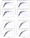 |
Fig. A.1 Model fits of scattered light to the VYSOS B and R band data in LDN 1780. Models are shown for four different forward scattering parameters, g = 0, 0.50, 0.75, and 0.90, and a range of albedos a as indicatedin the figures. The blue lines are for albedos in regular steps of 0.1 and the red lines for an intermediate a, given as the last one in the list of a values. The surface brightness is in units of 10−9 erg cm−2 s−1 sr−1 Å−1. |
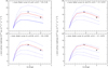 |
Fig. A.2 Model fits of scattered light to the two u band Calar Alto photometric data points in LDN 1780, indicated with crosses (see Table 6). Models are shown for four different forward scattering parameters, g = 0, 0.5, 0.75, and 0.90, and a range of albedos as indicated in the figures. The blue lines are for albedos in regular steps of 0.1 and the red lines for an intermediate a, given as the last one in the list of a values. The surface brightness is in units of 10−9 erg cm−2 s−1 sr−1 Å−1. |
Appendix B FUV and NUV scattered light model fits
In this Appendix we present the model fits of the observed surface brightnesses (scattered light) for LDN 1780 and the Draco nebula for the GALEX near and far UV wavelength bands, λ = 1771−2831Å and λ = 1344−1786Å.
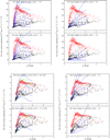 |
Fig. B.1 Model fits of scattered light to the Galex NUV and FUV band data in LDN 1780. Models are shown for four different forward scattering parameters, g = 0, 0.50, 0.75, and 0.90, and a range of albedos in regular steps of 0.1 (blue lines) and for an intermediate a (green line), given as the last one in the list of a values.The surface brightness is in units of 10−9 erg cm−2 s−1 sr−1 Å−1. |
 |
Fig. B.2 Model fits of scattered light to the Galex NUV and FUV band data in the Draco nebula. Models are shown for four different forward scattering parameters, g = 0, 0.50, 0.75, and 0.90, and a range of albedos in steps of 0.1, as indicated in the figures. The blue lines are for albedos in regular steps of 0.1. The surface brightness is in units of 10−9 erg cm−2 s−1 sr−1 Å−1. |
References
- Black, J. H., & van Dishoeck, E. F. 1987, ApJ, 322, 412 [NASA ADS] [CrossRef] [Google Scholar]
- Boksenberg, A., Evans, R. G., Fowler, R. G., et al. 1973, MNRAS, 163, 291 [NASA ADS] [Google Scholar]
- Cardelli, J. A., Clayton, G. C., & Mathis, J. S. 1989, ApJ, 345, 245 [NASA ADS] [CrossRef] [Google Scholar]
- Chlewicki, G., & Laureijs, R. J. 1987, NATO Adv. Sci. Inst. Ser. C, 191, 33 [Google Scholar]
- Choi, Y.-J., Min, K.-W., & Seon, K.-I. 2015, ApJ, 800, 132 [NASA ADS] [CrossRef] [Google Scholar]
- Cohen, M., Anderson, C. M., Cowley, A., et al. 1975, ApJ, 196, 179 [NASA ADS] [CrossRef] [Google Scholar]
- del Burgo, C., & Cambrésy, L. 2006, MNRAS, 368, 1463 [NASA ADS] [CrossRef] [Google Scholar]
- de Oliveira-Costa, A., Tegmark, M., Finkbeiner, D. P., et al. 2002, ApJ, 567, 363 [NASA ADS] [CrossRef] [Google Scholar]
- de Zeeuw, P. T., Hoogerwerf, R., de Bruijne, J. H. J., Brown, A. G. A., & Blaauw, A. 1999, AJ, 117, 354 [NASA ADS] [CrossRef] [Google Scholar]
- Draine, B. T. 1978, ApJS, 36, 595 [NASA ADS] [CrossRef] [Google Scholar]
- Draine, B. T. 2003, ApJ, 598, 1017 [NASA ADS] [CrossRef] [Google Scholar]
- Draine, B. T., & Lee, H. M. 1984, ApJ, 285, 89 [Google Scholar]
- Duley, W. W. 1987, MNRAS, 229, 203 [NASA ADS] [CrossRef] [Google Scholar]
- Duley, W. W., & Williams, D. A. 1980, ApJ, 242, L179 [NASA ADS] [CrossRef] [Google Scholar]
- Edelstein, J., Min, K.-W., Han, W., et al. 2006a, ApJ, 644, L153 [NASA ADS] [CrossRef] [Google Scholar]
- Edelstein, J., Korpela, E. J., Adolfo, J., et al. 2006b, ApJ, 644, L159 [NASA ADS] [CrossRef] [Google Scholar]
- Gladders, M. D., López-Cruz, O., Yee, H. K. C., & Kodama, T. 1998, ApJ, 501, 571 [NASA ADS] [CrossRef] [Google Scholar]
- Goerigk, W., Mebold, U., Reif, K., Kalberla, P. M. W., & Velden, L. 1983, A&A, 120, 63 [NASA ADS] [Google Scholar]
- Gondhalekar, P. M. 1990, The Galactic and Extragalactic Background Radiation, 139, 49 [NASA ADS] [CrossRef] [Google Scholar]
- Gondhalekar, P. M., Phillips, A. P., & Wilson, R. 1980, A&A, 85, 272 [NASA ADS] [Google Scholar]
- Gordon, K. D. 2004, Astrophysics of Dust, ASP Conf. Ser., 309, 77 [NASA ADS] [Google Scholar]
- Gordon, K. D., Witt, A. N., Carruthers, G. R., Christensen, S. A., & Dohne, B. C. 1994, ApJ, 432, 641 [NASA ADS] [CrossRef] [Google Scholar]
- Gordon, K. D., Witt, A. N., & Friedmann, B. C. 1998, ApJ, 498, 522 [NASA ADS] [CrossRef] [Google Scholar]
- Górski, K. M., Hivon, E., Banday, A. J., et al. 2005, ApJ, 622, 759 [NASA ADS] [CrossRef] [Google Scholar]
- Green, G. M., Schlafly, E. F., Finkbeiner, D. P., et al. 2015, ApJ, 810, 25 [NASA ADS] [CrossRef] [Google Scholar]
- Greenberg, J. M. 1986, Ap&SS, 128, 3 [NASA ADS] [CrossRef] [Google Scholar]
- Greenstein, J. L., Oke, J. B., Richstone, D., van Altena, W. F., & Steppe, H. 1977, ApJ, 218, L21 [NASA ADS] [CrossRef] [Google Scholar]
- Griffin, M. J., Abergel, A., Abreu, A., et al. 2010, A&A, 518, L3 [Google Scholar]
- Haas, M., Hackstein, M., Ramolla, M., et al. 2012, Astron. Nachr., 333, 706 [NASA ADS] [Google Scholar]
- Hauser, M. G., Arendt, R. G., Kelsall, T., et al. 1998, ApJ, 508, 25 [NASA ADS] [CrossRef] [Google Scholar]
- Henyey, L. G., & Greenstein, J. L. 1941, ApJ, 93, 70 [NASA ADS] [CrossRef] [Google Scholar]
- Hurwitz, M. 1994, ApJ, 433, 149 [NASA ADS] [CrossRef] [Google Scholar]
- Hoyle, F., & Wickramasinghe, N. C. 1969, Nature, 223, 459 [NASA ADS] [CrossRef] [Google Scholar]
- Ingalls, J. G., Bania, T. M., Boulanger, F., et al. 2011, ApJ, 743, 174 [NASA ADS] [CrossRef] [Google Scholar]
- Jo, Y.-S., Min, K.-W., Seon, K.-I., Edelstein, J., & Han, W. 2011, ApJ, 738, 91 [NASA ADS] [CrossRef] [Google Scholar]
- Jo, Y.-S., Seon, K.-I., Min, K.-W., Edelstein, J., & Han, W. 2017, ApJS, 231, 21 [NASA ADS] [CrossRef] [Google Scholar]
- Jones, A. P. 1988, MNRAS, 234, 209 [NASA ADS] [Google Scholar]
- Jones, A. P., Köhler, M., Ysard, N., et al. 2016, A&A, 588, A43 [NASA ADS] [CrossRef] [EDP Sciences] [Google Scholar]
- Kelsall, T., Weiland, J. L., Franz, B. A., et al. 1998, ApJ, 508, 44 [NASA ADS] [CrossRef] [Google Scholar]
- Kessler, M. F., Steinz, J. A., Anderegg, M. E., et al. 1996, A&A, 315, L27 [NASA ADS] [Google Scholar]
- Lai, T. S.-Y., Witt, A. N., & Crawford, K. 2017, MNRAS, 469, 4933 [NASA ADS] [CrossRef] [Google Scholar]
- Landolt, A. U. 2007, AJ, 133, 2502 [NASA ADS] [CrossRef] [Google Scholar]
- Laureijs, R. J., Mattila, K., & Schnur, G. 1987, A&A, 184, 269 [NASA ADS] [Google Scholar]
- Laureijs, R. J., Fukui, Y., Helou, G., et al. 1995, ApJS, 101, 87 [NASA ADS] [CrossRef] [Google Scholar]
- Lee, D.-H., Yuk, I.-S., Jin, H., et al. 2006, ApJ, 644, L181 [NASA ADS] [CrossRef] [Google Scholar]
- Lee, D.-H., Pak, S., Dixon, W. V. D., & van Dishoeck, E. F. 2007, ApJ, 655, 940 [NASA ADS] [CrossRef] [Google Scholar]
- Lee, D.-H., Seon, K.-I., Min, K. W., et al. 2008, ApJ, 686, 1155 [NASA ADS] [CrossRef] [Google Scholar]
- Lehtinen, K., & Mattila, K. 2013, A&A, 549, A91 [NASA ADS] [CrossRef] [EDP Sciences] [Google Scholar]
- Lehtinen, K., Russeil, D., Juvela, M., Mattila, K., & Lemke, D. 2004, A&A, 423, 975 [NASA ADS] [CrossRef] [EDP Sciences] [Google Scholar]
- Leinert, C., Väisänen, P., Mattila, K., Lehtinen, K. 1988, A&AS, 112, 99 [NASA ADS] [Google Scholar]
- Lemke, D., Klaas, U., Abolins, J., et al. 1996, A&A, 315, L64 [NASA ADS] [Google Scholar]
- Liljestrom, T.,& Mattila, K. 1988, A&A, 196, 243 [NASA ADS] [Google Scholar]
- Lillie, C. F., & Witt, A. N. 1976, ApJ, 208, 64 [Google Scholar]
- Lim, T.-H., Jo, Y.-S., Seon, K.-I., & Min, K.-W. 2015, MNRAS, 449, 605 [NASA ADS] [CrossRef] [Google Scholar]
- Liszt, H. S., Pety, J., & Tachihara, K. 2009, A&A, 499, 503 [NASA ADS] [CrossRef] [EDP Sciences] [Google Scholar]
- Lombardi, M., Alves, J., & Lada, C. J. 2011, A&A, 535, A16 [NASA ADS] [CrossRef] [EDP Sciences] [Google Scholar]
- Lombardi, M., Bouy, H., Alves, J., & Lada, C. J. 2014, A&A, 566, A45 [NASA ADS] [CrossRef] [EDP Sciences] [Google Scholar]
- Lynds, B. T. 1962, ApJS, 7, 1 [NASA ADS] [CrossRef] [Google Scholar]
- Lynds, B. T. 1965, ApJS, 12, 163 [NASA ADS] [CrossRef] [Google Scholar]
- Malinen, J., Juvela, M., Zahorecz, S., et al. 2014, A&A, 563, A125 [NASA ADS] [CrossRef] [EDP Sciences] [Google Scholar]
- Martin, C., Hurwitz, M., & Bowyer, S. 1990, ApJ, 354, 220 [NASA ADS] [CrossRef] [Google Scholar]
- Martin, D. C., Seibert, M., Buat, V., et al. 2005, ApJ, 619, L59 [NASA ADS] [CrossRef] [Google Scholar]
- Massey, P., Strobel, K., Barnes, J. V., Anderson, E. 1988, ApJ, 328, 315 [NASA ADS] [CrossRef] [Google Scholar]
- Mathis, J. S., Rumpl, W., & Nordsieck, K. H. 1977, ApJ, 217, 425 [NASA ADS] [CrossRef] [Google Scholar]
- Mathis, J. S. 1990, ARA&A, 28, 37 [NASA ADS] [CrossRef] [Google Scholar]
- Mattila, K. 1970a, A&A, 8, 273 [NASA ADS] [Google Scholar]
- Mattila, K. 1970b, A&A, 9, 53 [NASA ADS] [Google Scholar]
- Mattila, K. 1979, A&A, 78, 253 [NASA ADS] [Google Scholar]
- Mattila, K. 1990, The Galactic and Extragalactic Background Radiation, 139, 257 [NASA ADS] [CrossRef] [Google Scholar]
- Mattila, K., & Sandell, G. 1979, A&A, 78, 264 [NASA ADS] [Google Scholar]
- Mattila, K., Väisänen, P., & Appen-Schnur, G. F. O. V. 1996, A&AS, 119, 153 [NASA ADS] [CrossRef] [EDP Sciences] [Google Scholar]
- Mattila, K., Juvela, M., & Lehtinen, K. 2007, ApJ, 654, L131 [NASA ADS] [CrossRef] [Google Scholar]
- Mattila, K., Lehtinen, K., Väisänen, P., von Appen-Schnur, G., & Leinert, C. 2017, MNRAS, 470, 2133 [NASA ADS] [CrossRef] [Google Scholar]
- Mebold, U., Cernicharo, J., Velden, L., et al. 1985, A&A, 151, 427 [Google Scholar]
- Miville-Deschênes, M.-A., Salomé, Q., Martin, P. G., et al. 2017, A&A, 599, A109 [NASA ADS] [CrossRef] [EDP Sciences] [Google Scholar]
- Murthy, J. 2014, ApJS, 213, 32 [NASA ADS] [CrossRef] [Google Scholar]
- Murthy, J. 2016, MNRAS, 459, 1710 [NASA ADS] [CrossRef] [Google Scholar]
- Neufeld, D. A., & Spaans, M. 1996, ApJ, 473, 894 [NASA ADS] [CrossRef] [Google Scholar]
- Park, S.-J., Min, K.-W., Seon, K.-I., et al. 2009, ApJ, 700, 155 [NASA ADS] [CrossRef] [Google Scholar]
- Penprase, B. E., & Blades, J. C. 2000, ApJ, 535, 293 [NASA ADS] [CrossRef] [Google Scholar]
- Perryman, M. A. C., Lindegren, L., Kovalevsky, J., et al. 1997, A&A, 323, L49 [NASA ADS] [Google Scholar]
- Pickles, A. J. 1998, PASP, 110, 863 [CrossRef] [Google Scholar]
- Pilbratt, G. L., Riedinger, J. R., Passvogel, T., et al. 2010, A&A, 518, L1 [CrossRef] [EDP Sciences] [Google Scholar]
- Pineda, J. E., Caselli, P., & Goodman, A. A. 2008, ApJ, 679, 481 [NASA ADS] [CrossRef] [Google Scholar]
- Planck Collaboration XI. 2014, A&A, 571, A11 [NASA ADS] [CrossRef] [EDP Sciences] [Google Scholar]
- Ridderstad, M., Juvela, M., Lehtinen, K., Lemke, D., & Liljeström, T. 2006, A&A, 451, 961 [NASA ADS] [CrossRef] [EDP Sciences] [Google Scholar]
- Ryu, K., Min, K. W., Seon, K.-I., et al. 2008, ApJ, 678, L29 [NASA ADS] [CrossRef] [Google Scholar]
- Sandage, A. 1976, AJ, 81, 954 [NASA ADS] [CrossRef] [Google Scholar]
- Sandell, G., Johansson, L. E. B., Rieu, N. Q., & Mattila, K. 1981, A&A, 97, 317 [NASA ADS] [Google Scholar]
- Sandell, G., Reipurth, B., & Gahm, G. 1987, A&A, 181, 283 [NASA ADS] [Google Scholar]
- Schlafly, E. F., & Finkbeiner, D. P. 2011, ApJ, 737, 103 [NASA ADS] [CrossRef] [Google Scholar]
- Schlafly, E. F., Green, G., Finkbeiner, D. P., et al. 2014, ApJ, 789, 15 [NASA ADS] [CrossRef] [Google Scholar]
- Schmidt, G. D., Cohen, M., & Margon, B. 1980, ApJ, 239, L133 [NASA ADS] [CrossRef] [Google Scholar]
- Seon, K.-I., Edelstein, J., Korpela, E., et al. 2011, ApJS, 196, 15 [NASA ADS] [CrossRef] [Google Scholar]
- Smith, T. L., & Witt, A. N. 2002, ApJ, 565, 304 [NASA ADS] [CrossRef] [Google Scholar]
- Struve, O., & Zebergs, V. 1962, Astronomy of the 20th Century (New York: Macmillan), 399 [Google Scholar]
- Sujatha, N. V., Chakraborty, P., Murthy, J., & Henry, R. C. 2004, Bullet. Astron. Soc. Ind., 32, 151 [NASA ADS] [Google Scholar]
- Sujatha, N. V., Murthy, J., Suresh, R., Conn Henry, R., & Bianchi, L. 2010, ApJ, 723, 1549 [NASA ADS] [CrossRef] [Google Scholar]
- Thompson, G. I., Nandy, K., Jamar, C., et al. 1978, Catalogue of stellar ultraviolet fluxes. A compilation of absolute stellar fluxes measured by the Sky Survey Telescope (S2/68) aboard the ESRO satellite TD − 1, Science Research Council [Google Scholar]
- Togi, A., Witt, A. N., & John, D. S. 2017, A&A, 605, A99 [NASA ADS] [CrossRef] [EDP Sciences] [Google Scholar]
- Toller, G. N. 1981, Ph.D. Thesis, SUNY Stony Brook [Google Scholar]
- Toth, L. V., Haikala, L. K., Liljestroem, T., & Mattila, K. 1995, A&A, 295, 755 [NASA ADS] [Google Scholar]
- van Dishoeck, E. F., & Black, J. H. 1986, ApJS, 62, 109 [NASA ADS] [CrossRef] [Google Scholar]
- van Leeuwen, F. 2007, Astrophysics and Space Science Library, 350 [Google Scholar]
- Vidal, M., Casassus, S., Dickinson, C., et al. 2011, MNRAS, 414, 2424 [NASA ADS] [CrossRef] [Google Scholar]
- Weinberg, J. L., Hanner, M. S., Beeson, D. E., DeShields, L. M., II, & Green, B. A. 1974, J. Geophys. Res., 79, 3665 [NASA ADS] [CrossRef] [Google Scholar]
- Weingartner, J. C., & Draine, B. T. 2001, ApJ, 548, 296 [NASA ADS] [CrossRef] [Google Scholar]
- Whitworth, A. P. 1975, Ap&SS, 34, 155 [NASA ADS] [CrossRef] [Google Scholar]
- Witt, A. N., & Vijh, U. P. 2004, Astrophysics of Dust, ASP Conf. Ser., 309, 115 [NASA ADS] [Google Scholar]
- Witt, A. N., Schild, R. E., & Kraiman, J. B. 1984, ApJ, 281, 708 [NASA ADS] [CrossRef] [Google Scholar]
- Witt, A. N., Stecher, T. P., Boroson, T. A., & Bohlin, R. C. 1989, ApJ, 336, L21 [NASA ADS] [CrossRef] [Google Scholar]
- Witt, A. N., Friedmann, B. C., & Sasseen, T. P. 1997, ApJ, 481, 809 [NASA ADS] [CrossRef] [Google Scholar]
- Witt, A. N., Mandel, S., Sell, P. H., Dixon, T., & Vijh, U. P. 2008, ApJ, 679, 497 [NASA ADS] [CrossRef] [Google Scholar]
- Witt, A. N., Gold, B., Barnes, F. S., et al. 2010, ApJ, 724, 1551 [NASA ADS] [CrossRef] [Google Scholar]
- Wyman, K., & Redfield, S. 2013, ApJ, 773, 96 [NASA ADS] [CrossRef] [Google Scholar]
- Ysard, N., Köhler, M., Jones, A., et al. 2016, A&A, 588, A44 [NASA ADS] [CrossRef] [EDP Sciences] [Google Scholar]
- Zacharias, N., Monet, D. G., Levine, S. E., et al. 2004, Bull. Am. Astron. Soc., 36, 48 [Google Scholar]
- Zacharias, N., Monet, D. G., Levine, S. E., et al. 2005, ViZieR Online Data Catalog: I/1297 [Google Scholar]
- Zari, E., Lombardi, M., Alves, J., Lada, C. J., & Bouy, H. 2016, A&A, 587, A106 [NASA ADS] [CrossRef] [EDP Sciences] [Google Scholar]
Available at the address https://archive.stsci.edu/prepds/uv-bkgd/.
hspirepsw447_30pxmp_1539_m0706_1476933801545.fits, centre RA = 234.76159 deg, Dec = − 7.1134 deg (J2000), map size ~ 1. °8 × 1. °8, start date 210-18-04T11:00:13.
See also the updated compilation in Karl D. Gordon’s web page http://www.stsci.edu/~kgordon/Dust/Scat_Param/scat_data.html.
All Tables
Some basic properties of the sample of dark nebulae and the additional UV sources of illumination for LDN 1780.
Positions in Draco and LDN 1780: Calar Alto intermediate-band photometry and VYSOS surface brightness imaging.
NIR and optical extinction vs. thermal dust emission for four molecular clouds and for the high-latitude diffuse medium.
The Milky Way mean surface brightness as seen from a vantage point at z = 50 pc and z = 400 pc above the Galactic plane relative to the surface brightness at z = 0.
Intensity ratios of Milky Way surface brightness in different filter bands relative to B_ Pioneer and R_ Pioneer filter bands.
Parameters related to the ISRF attenuation, foreground extinction, and the off-cloud DGL models for fitting the LDN 1780 and LDN 1642 surface brightness observations.
All Figures
|
Fig. 1 Differential spectral energy distributions I(nebula) minus I(sky) for selected positions in LDN 1780 and the Draco nebula. The observed values are from Calar Alto photometry as described in Sect 2.1 and given in Table 3. |
| In the text | |
|
Fig. 2 LDN 1780 data. Upper left panel: B band VYSOS image with Calar Alto photometry positions shown as circles, the ISOPHOT 200 μm map area shown as rectangle and the two surface brightness “zero” areas as rectangles; contours are at 30.0, 23.75, 17.5, 11.25, and 5.0 ×10⁻⁹ erg cm−2 s−1 sr−1 Å−1. Upper right panel: GALEX FUV map; middle right panel: GALEX NUV map; middle left panel: map of H I 21-cm excess emission (line area), adopted from Mattila & Sandell (1979) Fig. 5; bottom left panel: SPEAR/FIMS H2 fluorescence emission map; bottom right panel: SPEAR/FIMS spectrum at RA = 15h 42m (235. °5), Dec = − 7. °4 (J2000), the brightest H2 spot in the cloud. In the GALEX images some artefacts of the 1. °25 field edges are seen as black arcs; the contours of the B band image are overplotted in the GALEX and SPEAR/FIMS for reference. Coordinates for the H I 21-cm map are RA and Dec (B1950.0); approximate J2000 coordinates have been added in red. The AB = 0. m5 extinction contour is shown as a dashed line. For the colour bars of the GALEX images and for the SPEAR/FIMS spectrum the unit is ph s−1 cm−2 sr−1 Å−1; for the colour bar of the SPEAR/FIMS H2 image the unit is ph s−1 cm−2 sr−1 (=LU, line unit). |
| In the text | |
|
Fig. 3 VYSOS i band image of LDN 1642; most stars have been removed. The La Silla photometry positions that are within this image area are shown as circles. |
| In the text | |
|
Fig. 4 Draco nebula images. Upper left panel: broad band optical; upper right panel: Herschel 250 μm; bottom left panel: GALEX FUV; bottom right panel: GALEX NUV. The 250 μm contours at 3, 6.6, 11, and 17 MJy sr−1 are shown and are also overplotted on the FUV and NUV images. They correspond to AV values of ~0.15, 0.36, 0.57, and 0.78 mag. The unit in the FUV and NUV colour bars is ph s−1 cm−2 sr−1 Å −1. Pixel size forFUV and NUV is 3′. At Eastern edge of the UV images the tip of the Sujatha et al. (2010) foreground filament is seen. The black area on the Western edge has no FUV and NUV data. Some artefacts of the GALEX 1. °25 field edges remain. The optical image was provided by Jim Thommes. |
| In the text | |
|
Fig. 5 VYSOS BV Ri surface brightness vs. visual extinction in LDN 1780. The relationships are shown from bottom to top in different colous: B (blue dots), V (green, shifted by +20 units), R (red, shifted by +40 units), and i (magenta, shifted by +60 units). The black crosses at AV = 0.43 mag indicate the zero level for each surface brightness band. |
| In the text | |
|
Fig. 6 Surface brightness vs. visual extinction in LDN 1642. The relationships are shown from bottom to top for: 3500 Å (u) (black dots), 3840 Å (magenta, shifted by +20 units), 4160 Å (black dots, +40 units), 4670 Å (b) (blue dots, +60 units), 5470 Å (green dots, +80 units), and 7478 Å (i) (red dots). The crosses at AV = 0.27 mag indicate the zero level for each surface brightness band. |
| In the text | |
|
Fig. 7 Surface brightness vs. visual extinction in the Draco nebula. The relationships are shown from bottom to top in different colours: 3500 Å (u) (black dots), 3920 Å (magenta, shifted by +20 units), 4030 Å (blue dots, +40 units), 4670 Å (b) (blue dots, +60 units), 5250 Å (black dots, +80 units), and 5800 Å (red dots, +100 units). The crosses at AV = 0.07 mag indicate the zero level for each surface brightness band. To guide the eye approximate linear fits are shown as dashed lines. Data for positions 1 and 3 (see Table 3) deviate by more than 3σ in most colours and are not shown in this plot. |
| In the text | |
|
Fig. 8 GALEX NUV (upper panel) and FUV (lower panel) surface brightness in LDN 1780 plotted against visual extinction. The red dots are for the southern (Dec < − 7°12′), the black dots for the northern (Dec ≥−7°12′) part of the cloud (RA < 15h 41.2m for both). |
| In the text | |
|
Fig. 9 GALEX NUV (upper panel) and FUV (lower panel) surface brightness in Draco nebula plotted against visual extinction. Red points are for the “Head” at l = 88.8−90.2 deg, b = 38.0−38.5 deg (see Fig. 4) and black points for the “Tail” part of the nebula. |
| In the text | |
|
Fig. 10 Albedo values vs. asymmetry parameter g derived from modelling as shown in Fig. A.1. Results are shown for LDN 1780 (blue symbols), LDN 1642 (black), and Draco nebula (red). For reference also the results for the Coalsack are shown in the UBV bands (green lines) (Mattila 1970b). |
| In the text | |
|
Fig. 11 Our derived dust albedos according to results shown in Figs. 10 and 13 and Table 9. For the black dots with error bars the g-parameter value of 0.80 has been adopted for all bands. For FUV and NUV albedos also the values for g = 0.50 are shown asblue point with error bars. For FUV (λ1540Å) and NUV (λ2320Å) the mean of LDN 1780 and Draco nebula is shown, with the Draco value at the lower and LDN 1780 value at the upper end of the error bar. Dust model albedo values are shown according to Draine (2003) (red curve), THEMIS CM (magenta), and THEMIS CMM (green) (Jones et al. 2016). |
| In the text | |
|
Fig. 12 FUVvs. NUV surface brightness in LDN 1780 (lower panel) and Draco nebula (upper panel). The southern part of LDN 1780 and the “Head” of Draco are indicated with red and the northern part of LDN 1780 and “other” parts of Draco with black dots (see Figs. 8 and 9). The mean intensity ratio for the all-sky diffuse background radiation according to Murthy (2014) is shown as the green line. |
| In the text | |
|
Fig. 13 Albedo values vs. asymmetry parameter g derived from modelling as shown in Figs. B.1 and B.2. Results are shown for LDN 1780 (blue symbols), and Draco nebula (red). |
| In the text | |
|
Fig. 14 Spectral energy distributions for Pos. 1 (upper left and upper right panels) and Pos. 10 (middle left and middle right panels)in LDN 1780, and Pos. 11 and 13 and mean of Pos. 6 and 8 in Draco nebula (bottom left panel). Observations are as in Fig. 1, model curves are according to starlight models (see text). |
| In the text | |
|
Fig. 15 FUV continuum and H2 fluorescence emission in LDN 1780; upper left panel: SPEAR/FIMS FUV continuum map with B band surface brightnes contours overlayed; upper right panel: the SPEAR/FIMS H2 fluorescence emission map + B band contours; lower left panel: total (red line) and continuum (blue dashed line) intensities shown as function of the declination along the path from south to north; lower right panel: H2 intensity(red line) and its statistical error (blue dashed line) along the same path across LDN 1780. The intensity unit for the total and continuum is photons cm−2 s−1 sr−1 Å−1 (CU; continuum unit) and for the line emission photons cm−2 s−1 sr−1 (LU; line unit). |
| In the text | |
|
Fig. 16 Upper panel: GALEX NUV; lower panel: FUV intensity in LDN 1780 as a function of HI 21-cm excess line area, adopted from Fig. 5 of Mattila & Sandell (1979). |
| In the text | |
|
Fig. 17 Left panel: extinction-corrected spectrum at the FUV peak region (black histogram) and the best-fit model spectrum forIUV = 1.7 (red line). Red dashed line indicates continuum level; (right panel) as in the left-hand panel but with models for IUV = 0.5, 1.0, 1.5, 1.7 (red line), 2.0, 2.5, and 3.0. |
| In the text | |
|
Fig. A.1 Model fits of scattered light to the VYSOS B and R band data in LDN 1780. Models are shown for four different forward scattering parameters, g = 0, 0.50, 0.75, and 0.90, and a range of albedos a as indicatedin the figures. The blue lines are for albedos in regular steps of 0.1 and the red lines for an intermediate a, given as the last one in the list of a values. The surface brightness is in units of 10−9 erg cm−2 s−1 sr−1 Å−1. |
| In the text | |
|
Fig. A.2 Model fits of scattered light to the two u band Calar Alto photometric data points in LDN 1780, indicated with crosses (see Table 6). Models are shown for four different forward scattering parameters, g = 0, 0.5, 0.75, and 0.90, and a range of albedos as indicated in the figures. The blue lines are for albedos in regular steps of 0.1 and the red lines for an intermediate a, given as the last one in the list of a values. The surface brightness is in units of 10−9 erg cm−2 s−1 sr−1 Å−1. |
| In the text | |
|
Fig. B.1 Model fits of scattered light to the Galex NUV and FUV band data in LDN 1780. Models are shown for four different forward scattering parameters, g = 0, 0.50, 0.75, and 0.90, and a range of albedos in regular steps of 0.1 (blue lines) and for an intermediate a (green line), given as the last one in the list of a values.The surface brightness is in units of 10−9 erg cm−2 s−1 sr−1 Å−1. |
| In the text | |
|
Fig. B.2 Model fits of scattered light to the Galex NUV and FUV band data in the Draco nebula. Models are shown for four different forward scattering parameters, g = 0, 0.50, 0.75, and 0.90, and a range of albedos in steps of 0.1, as indicated in the figures. The blue lines are for albedos in regular steps of 0.1. The surface brightness is in units of 10−9 erg cm−2 s−1 sr−1 Å−1. |
| In the text | |
Current usage metrics show cumulative count of Article Views (full-text article views including HTML views, PDF and ePub downloads, according to the available data) and Abstracts Views on Vision4Press platform.
Data correspond to usage on the plateform after 2015. The current usage metrics is available 48-96 hours after online publication and is updated daily on week days.
Initial download of the metrics may take a while.