© ESO 2018

1 Introduction

Supermassive black holes (SMBHs) at the center of galaxies grow through the accretion of nearby matter and a fraction of the gravitational potential of the accreted mass is converted into radiation. In this case the SMBH is called an active galactic nucleus (AGN). The idea of a possible connection between the growth of the SMBH and the evolution of its host galaxy was put forward, once a correlation between black hole mass (M_BH) and the bulge luminosity was discovered (Kormendy & Richstone 1995; Silk & Rees 1998; Granato et al. 2004; Di Matteo et al. 2005; Menci et al. 2008). Since the energy released by the growth of the black hole can be larger than the binding energy of the galaxy bulge, the AGN can have an important effect on the evolution of its host galaxy. Indeed, fast winds can be launched from the accretion disk, collide with the interstellar medium (ISM), and drive powerful kiloparsec-scale outflows, which may sweep out the gas in the galaxy and then may be responsible for the regulation of the star formation and BH accretion (Zubovas & King 2012; Faucher-Giguère & Quataert 2012; Fabian 2012, see Fiore et al. 2017 for a detailed discussion).

Over the past few years efforts have been made to search for AGN outflows in different ISM phases. Evidence of radiatively-driven winds are observed at subparsec scale, in the innermost regions of the AGN through the detection of blueshifted, highly ionized Fe K-shell transitions, that is, ultra fast outflows (UFOs), with velocities ~ 0.2c (King & Pounds 2015; Tombesi et al. 2010, 2014; Gofford et al. 2013); at parsec scale via warm absorbers and broad absorption lines (BAL), moving at velocities up to 10 000 km s⁻¹ (King & Pounds 2015; Tombesi et al. 2013); at kpc scale through different gas phases such as ionized gas, that is, broad asymmetric blueward [OIII] emission lines (Harrison et al. 2012, 2014; Cano-Díaz et al. 2012; Brusa et al. 2015; Carniani et al. 2015); neutral atomic gas such as NaID (Rupke & Veilleux 2015), and molecular gas with velocities up to a few thousands km s⁻¹ (Feruglio et al. 2010; Cicone et al. 2014; Spoon et al. 2013). The investigation of the possible correlations of AGN properties over a wide range of spatial scales can give us more information about the nature of AGNs and the impact they have on their surroundings.

The most popular theoretical models of AGN-driven outflows (Faucher-Giguère & Quataert 2012) suggest that the kinetic energy of the nuclear fast outflows is transferred to the ISM and drive the kpc-scale flows, in a likely energy-conserving scenario. This has been reflected in the observations of both UFO and molecular winds in two sources, Markarian 231 (Feruglio et al. 2015) and IRASF11119+13257 (Tombesi et al. 2015, but see Veilleux et al. 2017).

The high ionization lines, such as CIVλ1549 Å, are known to exhibit asymmetric profiles toward the blue-side, with the peak of the emission line blueshifted with respect to the low ionization lines, such as MgII or Hβ (Gaskell 1982; Sulentic et al. 2000 and Richards et al. 2011). This behavior cannot be ascribed to virialized motion but it can be interpreted in terms of outflowing gas, which possibly leads to biased BH mass estimates derived from the entire CIV emission line (Denney 2012; Coatman et al. 2017).

The blueshift of the CIV emission line can be a valuable tool to trace the winds in the broad line region (BLR). The CIV emission line typically shows a blueshift of ~ 600 km s⁻¹ up to 2000 km s⁻¹ (Shen et al. 2011; Richards et al. 2002). The largest blueshifts have been discovered in an extreme quasar (QSO) population at 2.2 <~ z <~ 5.9, the so-called weak line QSOs (hereafter WLQs), which exhibit weak or undetectable ultraviolet (UV) emission lines, that is, they are defined as QSOs with a rest-frame equivalent width (REW) of the CIV emission line of less than 10 Å (Fan et al. 1999; Diamond-Stanic et al. 2009; Plotkin et al. 2010; Wu et al. 2011). The velocity shift of the CIV emission line correlates with several parameters of optical and ultraviolet emission lines. In particular itis part of 4D Eigenvector 1 parameter space (Boroson & Green 1992; Sulentic et al. 2000), which also involves the broad Fe II emission, the equivalent width of the narrow [OIII] component, the width of the Hβ emission line, and the X-ray photon index. The physical driver of the 4D Eigenvector 1 is thought to be the Eddington ratio (λ_Edd), since QSOsshowing large blueshifts accrete at high rate, with λ_Edd ≥ 0.2 (Marziani et al. 2001; Boroson 2002; Shen & Ho 2014).

As found by Marziani et al. (2016), these winds occurring in the BLR may affect the host galaxy. They studied a sample of QSOs with L_Bol = 10^45−48.1 erg s⁻¹ at 0.9 <~ z <~ 3 and found that the outflow kinetic power of these winds traced by the CIV emission line is comparable to the binding energy of the gas in a massive spheroid, underlining the importance of considering also these winds in the feedback scenario. It is therefore crucial to study such AGN-driven outflows at the golden epoch of AGN activity, for example, 1.5 < z < 3.5. Furthermore, from theory and observations we know that the efficiency in driving energetic winds increases with AGN luminosity (Menci et al. 2008; Faucher-Giguère & Quataert 2012), which brings out the need to investigate the properties of the most luminous QSOs.

We have undertaken a multiwavelength survey to investigate a sample of 86 Type-1 WISE/SDSS selected hyper-luminous AGNs (L_Bol > 2 × 10⁴⁷ erg s⁻¹; Duras et al., in prep.), known as the WISSH sample (see Bischetti et al. 2017 for further details, Paper I hereafter; Duras et al. 2017). In Paper I we discussed the discovery of extreme kpc-scale outflows in five WISSH QSOs, traced via the blueshift of the [OIII]λ5007 Å emission line. In this paper we report on the discovery of fast BLR winds (with velocities up to 8000 km s⁻¹) traced by the blueshift of the CIV with respect to the systemic redshift, and their possible relation with the narrow line region (NLR) winds. We concentrate the analysis on the first 18 WISSH QSOs with rest-frame optical observations and UV archival data at z ~ 2.2–3.6. In Sect. 2, we present details about the observations and data reduction of proprietary data, such as LBT/LUCI1 and VLT/SINFONI spectra, and archival data from SDSS DR10. In Sect. 3, we outline the models used in our spectral analysis and present the results of the spectral fit, both for optical and UV spectra. In Sect. 4.1, we discuss the properties of the [OIII] and Hβ emission lines in the context of a scenario based on the orientation of our line of sight. Eddington ratios and Hβ-based SMBH masses are presented in Sect. 4.2. We discuss the properties of the CIV emission line in Sect. 4.3, with particular emphasis on the blueshifted component and the mass outflow rate and kinetic power of the associated BLR winds in the WISSH QSOs, and their relation with NLR winds traced by [OIII]. In Sect. 5 we investigate the dependence of the CIV velocity shifts on fundamental AGN parameters such as L_Bol, λ_Edd, and the spectral index α_OX defined as $${\alpha }_{\text{OX}}=\frac{\text{Log}(L_{\text{2keV}}/L_{2500\AA })}{\text{Log}({\nu }_{\text{2keV}}/{\nu }_{2500\AA })}$$(1)

and representing the slope of a power law defined by the rest-frame monochromatic luminosities at 2 keV (L_2keV) and 2500 Å (L_{2500 Å}). Finally we summarize our findings in Sect. 6. Throughout this paper, we assume H₀ = 71 km s⁻¹ Mpc⁻¹, Ω_Λ = 0.73, and Ω_m = 0.27.

2 Observations and data reduction

We have collected near-infrared (NIR) spectroscopic observations for 18 WISSH QSOs. Five of them have been discussed in Paper I, while the properties of an additional 13 QSOs, with LUCI1/LBT (ten objects) and VLT/SINFONI (three objects) observations are presented in the present paper. The coordinates, SDSS tenth data release (DR10) redshift, optical photometric data (Ahn et al. 2014), 2MASS NIR photometric data (Skrutskie et al. 2006), and color excess E(B–V) derived from broadband SED fitting (Duras et al., in prep) of the WISSH QSOs analyzed here are listed in Table 1.

2.1 LUCI/LBT observations

The observations of ten WISSH QSOs were carried out with LUCI1, the NIR spectrograph and imager at the Large Binocular Telescope (LBT) located in Mount Graham, Arizona. We required medium resolution spectroscopic observations in longslit mode with a slit of 1 arcsec width, using the N1.8 camera. The gratings 150_K_s (R = 4140) in the K band and 210_zJHK (R = 7838) in H band were used for objects at redshift bins 2.1 < z < 2.4 and 3.1 < z < 3.6, respectively. The wavelength ranges covered are 1.50–1.75 μm and 1.95–2.40 μm for the H and K bands, respectively. The observations were performed from April 2014 to March 2015, in two different cycles. The average on-site seeing of both cycles is comparable, ~0.8 arcsec (see Table 2 for further details). Observations of stars with known spectral type were taken during the observing nights to account for telluric absorption and flux calibration.

The data reduction was performed using IRAF tasks and IDL routines on both targets and standard stars. The reduced final frames are calibrated in wavelength and flux and are free from sky lines and telluric absorption. We used argon and neon arc-lamps for the wavelength calibration of J0801+5210, J0958+ 2827, J1106+6400, J1157+2724, and J1201+0116; OH sky emission lines for the J1111+1336, J1236+6554, J1421+4633, and J1422+4417; and finally, argon and xenon arc-lamps for J1521+5202. For the lines’ identification, a cubic spline was used to fit the pixel coordinates to the wavelengths provided. Analysis of the night sky lines indicated an uncertainty in the wavelength calibration of ≲ 20 km s⁻¹. We performed an unweighted extraction of the 1D spectrum, using different apertures according to the spatial profile of each 2D spectrum, which was traced using a Chebyshev function of the 3rd order.

The sky subtraction was done by subtracting frames corresponding to different telescope pointings along the slit (ABBA method). To remove the atmospheric absorption features we used the IDL routine XTELLCOR_GENERAL (Vacca et al. 2003). This routine makes use of (i) the observed standard stars spectra, which are affected by telluric absorption as the targets, and (ii) a Vega model spectrum, useful to build up an atmospheric-absorption-free spectrum. As the magnitudes of the standard stars are also known, we calibrated the target spectra in absolute flux, with the same IDL routine.

2.2 SINFONI observations

Three QSOswere observed with Spectrograph for INtegral Field Observations in the Near Infrared (SINFONI), at the VLT installed at the Cassegrain focus of Unit Telescope 4 (UT4). The observations were performed in service mode during the period 093.A, with the adaptive optics (AO) - Laser Guide Star (LGS) mode, by which the atmospheric turbulence can be partially corrected. J1538+0855 and J2123–0050 were observed during the nights of Jul. 19 and Jul. 20 2014, while J2346−0016 was observed during Aug. 18 and Sept. 1 2014, as part of the program 093.A–0175. All the targets were observed within a field of view of 3′′ × 3′′, with a spaxel scale of 0.05′′ × 0.1′′. The final spatial resolution obtained thanks to the LGS correction is ~0.3′′ for J1538+0855 and J2346−0016, and ~ 0.2′′ for J2123–0050, as derived by the Hβ broad emission line. Given the redshift range of the QSOs, we used K and H filters to target the Hβ–[OIII]λ5007 Å spectral region with a resolving power of R ~ 4000 and 3000, respectively. The data reduction was performed using ESO pipelines, in Reflex environment (Freudling et al. 2013). The background sky emission was removed with the IDL routine SKYSUB, using object frames taken at different telescope pointings (see Davies 2007). After the cube reconstruction, the flux calibration was performed with our own IDL routines, by means of telluric spectra acquired during the same nights as the targets. As a final step, we extracted a 1D spectrum for each source with a circular aperture of 1′′ diameter. This procedure does not allow us to have the spatial information, but we are interested in the integrated emission from different AGN components (i.e., BLR and NLR). The analysis of the spatially-resolved kinematics of the [OIII]λ5007 emission line will be presented in a forthcoming paper. Detailed information about SINFONI observations are listed in Table 3.

2.3 SDSS archival data

We retrieved the rest-frame UV spectrum of the 18 WISSH QSOs with NIR spectroscopic data, from the Sloan Digital Sky Survey (SDSS) DR10 public archive, in order to derive the properties of the CIV emission line. The SDSS survey uses a dedicated wide-field 2.5 m telescope (Gunn et al. 2006) at Apache Point Observatory in Southern New Mexico. The spectra were obtained from February 2001 to February 2012 with two spectrographs, SDSS-I and BOSS, with a resolving power of 1500 at 3800 Å and 2500 at 9000 Å. The optical brightness of our objects, 15.6 < r< 18.25, ensures data with an excellent signal-to-noise ratio (>15) of the analyzed spectra.

3 Spectroscopic analysis

3.1 Modeling of the Hβ and [OIII] emission

The visual inspection of the rest-frame optical spectra of the 13 WISSH QSOs taken with LBT/LUCI or VLT/SINFONI revealed the weakness of the [OIII]λλ4959, 5007 Å doublet emission lines and the presence of a strong and complex FeII emission (see Appendix B). This combination makes the determination of [OIII] spectral parameters an extremely challenging task. In one case, that of J1422+4417, the LBT/LUCI1 bandwidth does not cover the [OIII] spectral region.

We developed a model based on the IDL package MPFIT (Markwardt 2009) in order to accurately infer the properties of the [OIII] and Hβ emission in these hyper-luminous QSOs. The NIR spectra were fitted with a spectral model which consists of:

Hβ/[OIII] core components associated with the NLR. Specifically, one Gaussian component for fitting the core of Hβ 4861 Å line with the full width at half maximum $FWH{M}_{\text{H}\beta }^{\text{core}}$ ≤ 1000¹ km s⁻¹ plus one Gaussian profile for each component of the [OIII]λλ4959, 5007 Å doublet. The FWHM of the [OIII] doublet was forced to be the same as that of the Hβ core component. Moreover, we assumed the theoretical flux ratio for [OIII]λλ4959, 5007 Å to be equal to 1:3 and the separation between [OIII]λλ4959–5007 Å and Hβ to be fixed to 98–146 Å in the rest frame, respectively.

[OIII] outflow components. Specifically, one Gaussian profile with the same FWHM for each component of the [OIII] in order to accurately constrain the possible presence of subtle broad or shifted components associated with outflows. Furthermore, we left free to vary the values of the FWHM ($FWH{M}_{[\text{OIII}]}^{\text{broad}}$) and centroids (${\lambda }_{[\text{OIII}]}^{\text{broad}}$) in the range 500–2500 km s⁻¹ and 4980–5034 Å, respectively, which are based on the values derived for these spectral parameters from the analysis of the [OIII] broad features in Paper I.

Hβ broad component associated with the BLR. Specifically, one Gaussian profile with width free to vary or a broken power-law (BPL) component convolved with a Gaussian curve (e.g., Nagao et al. 2006, Carniani et al. 2015, Paper I).

As in Paper I, in order to fit the prominent FeII emission, we included one or two Fe II templates depending on the complexity of the iron emission. Specifically, this was done by adding to the fit one or two templates chosen through the χ² minimization process among a library consisting of the three observational templates by Boroson & Green (1992), Véron-Cetty et al. (2004), and Tsuzuki et al. (2006), and twenty synthetic FeII templates obtained with the CLOUDY plasma simulation code (Ferland et al. 2013), which takes into account different hydrogen densities, ionizing photon densities, and turbulence. The FeII template was then convolved with a Gaussian function with a velocity dispersion σ in the range 500–4000 km s⁻¹. The continuum was fitted by a power-law component with the normalization left free to vary and the slope derived from the best-fit to the spectral energy distribution (SED) in the wavelength range of the observations. This parametrization worked well for all but two sources, J1538+0855 and J2123–0050, for which we used a slope left free to vary. We estimated the statistical noise from the line-free continuum emission and assumed it to be constant over the entire wavelength bandwidth. Finally, the uncertainty of each parameter has been evaluated considering the variation of χ² around the best fit value, with a grid step. From the corresponding χ² curve, we measured the Δχ² with respect to the minimum best-fit value. Hereafter, the reported errors refer to the one standard deviation confidence level, corresponding to Δχ² = 1 for each parameter of interest.

This fit yielded a good description of the observed NIR spectrum of the WISSH QSOs. The results of our spectral analysis for the Hβ and [OIII]λ5007 emission lines are listed in Table 4 and Table 5, respectively. Figure 1 shows an example of the Hβ and [OIII] spectral line fitting decomposition.

We estimated the spectroscopic redshift from the Hβ core component. The bulk of the Hβ emission is provided by the BLR component, which is well fitted by a broken power law for all but four cases (for J0801+5210, J0958+2827, J1422+4417, and J1521+5202 a Gaussian component was preferred). The FWHM of Hβ associated with the BLR has a range of 4000–8000 km s⁻¹, with a rest-frame equivalent width of 20–100 Å.

The normalization of the [OIII] emission line associated with the NLR is consistent with zero in all but three QSOs (namely J0958+2827, J1106+6400, and J1236+6554) with a $RE{W}_{[\text{OIII}]}^{\text{core}}$ ≈ 1 Å, confirming the weakness of this feature in the spectra considered here. Regarding the spectral components associated with a wind, for all but one of the QSOs (J1538+0855) the best value of their FWHMs or centroids is equal to the maximum or minimum value allowed by our model (500–2500 km s⁻¹ and 4980 Å, respectively), or the centroids fall extremely redward to 5007 Å (i.e. >5020 Å). The combination of these findings strongly suggests that this weak ($RE{W}_{[\text{OIII}]}^{\text{broad}}$ ≤ 3 Å) Gaussian component is likely to account for additional FeII emission not properly fitted by the templates, instead of these being due to a wind. In the case of J1538+0855, we measured a broad (${\mathrm{FWHM}}_{[\text{OIII}]}^{\text{broad}}$ = 1980 km s⁻¹), blueshifted ($v_{[\text{OIII}]}^{\text{broad}}$ = 1200 km s⁻¹) component with a $RE{W}_{[\text{OIII}]}^{\text{broad}}$ = 7.7 Å, making us highly confident in associating this spectral feature with blueshifted [OIII] emission. Hereafter, we refer to the “[OIII] sample” as the group of WISSH QSOs showing a REW of the [OIII] emission line ≥ 5 Å, while QSOs with $RE{W}_{[\text{OIII}]}^{\text{broad}}$ < 5 Å are included in the “Weak [OIII] sample”. Despite the fact that its NIR spectrum does not cover the [OIII] region, we also included the WISSH QSO J1422+4417 as a Weak [OIII] source, as it shows distinguishing features of this subclass (i.e. CIV velocity shift ~5000 km s⁻¹, see Sect. 3.2 and Table 6).

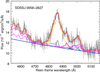Fig. 1 Parametrization of the Hβ-[OIII] region of the WISSH QSO J0958+2827. The red line shows the best fit to the data. Green curve refers to the core component associated with the NLR emission of Hβ and [OIII] emission lines. The blue curve refers to the broad blueshifted emission of [OIII]λλ4959, 5007 Å, indicative of outflow (but see Sect. 3.1 for more details). Gold curve indicates the broad component of Hβ associated with BLR emission. FeII emission is marked in magenta.

3.2 Modeling of the CIV emission

We shifted the SDSS spectra to the systemic rest frame using the redshift measured from the Hβ core component. The SDSS analysis was focused on the spectral region of the CIV emission line at 1549 Å, including spectral ranges free of emission or absorption features at both two sides of the CIV line centroid, in order to constrain the local underlying continuum. The CIV emission was fitted using a combination of up to three Gaussian profiles with spectral parameters (centroid, width, and normalization) left free to vary. We found that for all but three QSOs the best-fit model consists of a combination of two Gaussian components. For the BAL QSOs J1157+2724 and J1549+1245, for which the blue side of the CIV line profile is heavily affected by absorption, the CIV is modeled by one Gaussian component (see Fig. ?? for J1157+2724 and Fig. ?? for J1549+1245) and for the quasar J0745+4734, showing a very prominent peak at 1549 Å, the best-fit model of the CIV profile is the combination of three Gaussian components (see Fig. C.1).

We considered in our fits the presence of FeII emission by using UV FeII templates from Vestergaard & Wilkes (2001), although FeII is not particularly strong in the CIV region. These templates were convolved with Gaussian profiles of different widths to account for the observed FeII-related emission features in the spectra. If requested, we also included in the model one or two Gaussian components to account for HeIIλ1640 Å and/or OIII]λ1664 Å emissions.

The resulting physical parameters of the CIV emission for the 18 WISSH QSOs are listed in Table 6. We found a median value of REW_CIV = 21 Å with the lowest value for the object J1521+5202 (REW_CIV = 8 Å), confirming its WLQ nature (Just et al. 2007). The CIV emission profile is broad with a median value of FWHM_CIV = 7800 km s⁻¹ and, in four cases, exceptional values of FWHM_CIV (> 10 000 km s⁻¹) are detected. Moreover we found that the peak of the CIV profile is blueshifted with respect to the systemic redshift, with a velocity shift ($v_{\text{CIV}}^{\text{peak}}$ hereafter) in the range of $v_{\text{CIV}}^{\text{peak}}$ = 200–7500 km s⁻¹ in all cases except for J1326–0005, whose velocity shift is $v_{\text{CIV}}^{\text{peak}}$ = –50 km s⁻¹ (bearing in mind the presence of BAL features in this quasar).

The CIV emission line in the Weak [OIII] QSOs shows broad, strongly blue and asymmetric profiles, with $v_{\text{CIV}}^{\text{peak}}$ in the range of $v_{\text{CIV}}^{\text{peak}}$ = 2500–7500 km s⁻¹. This clearly indicates the presence of an outflowing component associated with this transition. According to the best-fit model, we refer to the Gaussian line with the most blueshifted centroid as the outflow component, with $v_{\text{CIV}}^{\text{out}}$ indicating its velocity shift with respect to the systemic redshift (see Fig. 2 upper panel).

The [OIII] sample exhibit the FWHM_CIV in the range of 2000–5000 km s⁻¹, and lower blueshifts than those of the Weak [OIII] QSOs, $v_{\text{CIV}}^{\text{peak}}$ ≤ 2000 km s⁻¹. The profile of the CIV line in [OIII] QSOs typically is more symmetric than in Weak [OIII] objects, indicating a dominant contributionfrom the emission of virialized gas. We therefore consider in this case the Gaussian component with the largest FWHM as the virialized one of the CIV emission line, while the second Gaussian component with a smaller FWHM is assumed to represent the emission associated with the wind (see Fig. 2 lower panel). It is worth noting that for the vast majority of our objects we measure a virialized component with a centroid not consistent (>2σ) with 1549 Å (see Appendix C). This can be interpreted in terms of a low-velocity component likely associated with a virialized flow in a rotating accretion disk wind (Young et al. 2007; Kashi et al. 2013). Finally, in the case of J1538+0855, an [OIII] object that also exhibits some distinctive properties of Weak [OIII] sources (see Appendix A), the virialized and outflow components of the CIV emission are assumed to be like those of Weak [OIII] sources.

Fig. 2 Parametrization of the CIV emission line profile of the Weak [OIII] quasar J1422+4417 (upper panel) and the [OIII] quasar J0745+4734 (lower panel). In both panels the red, yellow, and blue curves refer to the best fit of the spectrum, virialized component, and outflow component of the CIV emission line, respectively. The black dashed line indicates the λCIV at 1549 Å. The red dotted-dashed line denotes the peak of the CIV emission line and$v_{\text{CIV}}^{\text{peak}}$ represents its velocity shift with respect to the systemic λ1549 Å. The blue dotted-dashed line indicates the peak of the outflow component and $v_{\text{CIV}}^{\text{out}}$ is its velocity shift with respect to the systemic redshift. In the lower panel the green curve refers to an additional Gaussian component required by the fit, in order to better describe the CIV profile in this QSO.

4 Results

4.1 Properties of the [OIII] emission: REW_[OIII] and orientation

The observed equivalent width of the total profile of the [OIII] emission line (REW_[OIII]) can be used as an indicator of the line-of-sight inclination as found by Risaliti et al. (2011) and Bisogni et al. (2017a), that is, REW_[OIII] = REW_intrinsic∕cos(θ) (with θ as the angle between the accretion disk axis and the line of sight). In these works they showed that the distribution of REW_[OIII] of a large sample of SDSS DR7 AGN with 0.001 <  z  < 0.8, hereafter SDSS distribution, shows a power-law tail with a slope of –3.5 at the largest REW_[OIII] values, which is well reproduced by assuming an isotropic [OIII] emission (which is proportional to the intrinsic disk luminosity) and a random inclination of the accretion disk with respect to the line of sight. This demonstrates that the inclination effect is likely to be responsible for the large-REW_[OIII] power-law tail, whereby the higher the REW_[OIII], the higher the inclination.

The [OIII] sample of the WISSH QSOs exhibits REW_[OIII] ≈ 7–80 Å, which is mostly due to the broad blueshifted component of the [OIII] emission. Risaliti et al. (2011) and Bisogni et al. (2017a) reported that REW_[OIII] ≥ 25–30 Å are associated with nearly edge-on AGN. Half of [OIII] sources populate the high tail of the SDSS REW_[OIII] distribution with REW_[OIII] >~ 25 Å (Fig. 3 top). Therefore, a high inclination, θ ≈ 25°–73° (Bisogni et al. in prep.), can likely explain such large REW_[OIII].

The average value of REW_[OIII] for the Weak [OIII] sample is ≈2 Å. Given their high bolometric luminosities, weak [OIII] emission is expected in WISSH QSOs due to overionization of the circumnuclear gas as found in Shen & Ho (2014) by analyzing the rest-frame optical spectra of ~20 000 Type-1 SDSS QSOs. Another explanation for the reduced [OIII] emission could be linked to the ionization cone perpendicular to the galaxy disk, which would intercept a lower amount of ISM, resulting in a [OIII] line with a lower REW.

Furthermore, the [OIII] WISSH QSOs typically have higher REW_Hβ values than the Weak [OIII] sources (Fig.3, bottom), supporting a larger inclination scenario, which leads to an observed lower underlying continuum. We also note that the REW_Hβ distribution of the WISSH quasar is consistent with SDSS REW_Hβ distribution. As found in Bisogni et al. (2017a), we might expect a trend of the $FWH{M}_{\text{\_H}\beta }^{\text{BLR}}$ also for the WISSH QSOs, that is, the width of the Hβ increases from low to high inclination (from small EW_[OIII] to large EW_[OIII]). However, all the WISSH objects exhibit large values of $FWH{M}_{\text{\_H}\beta }^{\text{BLR}}$ and we do not observe any significant trend. This can be probably explained by the presence of ultra-massive BHs in these hyper-luminous AGN (see Sect. 4.2), which heavily dilute the effect of inclination.

If the inclination plays a role in explaining the large differences in REW_[OIII] between [OIII] and Weak [OIII] WISSH QSOs, we also expect differences in the near- and mid-IR SED, as found by Bisogni et al. (2017b) in a large SDSS sample of QSOs. Face-on QSOs offer a direct view of the hottest dust component located in the innermost part of the torus, while in case of high-inclination sources the view of this region can be partially blocked. This is consistent with the result obtained by comparing the average SEDs corresponding to WISE photometry of the QSOs in the [OIII] and Weak [OIII] samples (Fig. 4), where sources with high REW_[OIII] show a flux deficit in the NIR part of the SED, around 3 μm with respectto Weak [OIII] sources.

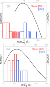Fig. 3 Observed distribution of the WISSH QSOs for the [OIII] and Weak [OIII] samples of (a) REW[OIII] and (b) REWH β, compared to the best fit of the REW[OIII] and REWHβ observed distribution of SDSS DR7 AGNs of Bisogni et al. (2017a) (black solid line).

Fig. 4 Average SEDs corresponding to WISE photometry of the WISSH [OIII] (dashed blue line) and Weak [OIII] samples (red line), normalized at 15 μm (dot-dashed line).

4.2 Single epoch Hβ-based SMBH masses and Eddington ratios

A common method of measuring black hole mass (M_BH) is the so-called single epoch technique (SE), which depends on BLR size estimated from the continuum luminosity of the quasar and on the velocity dispersion of the BLR, derived from the FWHM of a specific broad emission line, that is, Hα, Hβ, MgII, CIV, Paα, and Paβ depending on the redshift (McGill et al. 2008; Trakhtenbrot & Netzer 2012; Matsuoka et al. 2013; Ricci et al. 2017). As mentioned in Sect. 3.2, the CIV emission line is affected by the presence of non-virialized components (Baskin & Laor 2005; Richards et al. 2011), which can bias the BH mass estimation. The Hβ clouds are mostly dominated by virial motions, making this emission line the best estimator of the SMBH mass (Denney 2012). In order to estimate M_BH, we used the SE relation for Hβ reported in Bongiorno et al. (2014): $$\text{Log}(M_{\text{BH}}/M_{\odot })=6.7+2\times \text{Log}\left(\frac{FWHM}{{10}^3\text{\hspace{0.17em}km\hspace{0.17em}}{\text{s}}^{-1}}\right)+0.5\times \text{Log}\left(\frac{\lambda L_{\lambda }}{{10}^{44}\text{\hspace{0.17em}erg\hspace{0.17em}}{\text{s}}^{-1}}\right)$$(2)

For each quasar, we used the best-fit value of the FWHM of the broad component of Hβ line derived in Sect. 3 (see Table 4) and the continuum luminosity at 5100 Å. Both the L₅₁₀₀ and L_Bol were obtained byfitting the UV to mid-IR photometric data (see Table 1), with Type 1 AGN SED templates of Richards et al. (2006) using a Small Magellanic Cloud extinction law (Prevot et al. 1984)with color excess E(B–V) as free parameter (Duras et al. in prep.). We list the results of Hβ-based M_BH for all the WISSH QSOs with rest-frame optical spectroscopy in Table 7.

We found that all the BHs have masses larger than 10⁹ M_⊙, with nine out of 18 QSOs hosting SMBHs with M_BH >~ 5 × 10⁹ M_⊙. Based on these Hβ-based M_BH values and L_Bol, we derived Eddington ratios λ_Edd = L_Bol /L_Edd = 0.4–3.1 (with a median value of 1), where L_Edd = 1.26 × 10³⁸ (M_BH /M_⊙) erg s⁻¹, which are also reported in Table 7. For the WISSH [OIII] objects we also estimated the bolometric luminosity ($L_{\text{Bol}}^{\text{corr}}$) corrected for the orientation effect using the mean inclination angles as determined in Bisogni et al. (in prep.). Specifically, considering the expression for the observed REW_[OIII] distribution (Eq. (4) in Risaliti et al. 2011) as a function of the ratio between observed and intrinsic REW_[OIII], it is possible to retrieve the inclination angle probability distribution given the observed REW_[OIII] and, hence, the mean values of inclination angles.

Figure 5 shows the comparison of the M_BH, L_Bol, and λ_Edd measured for WISSH QSOs with those derived from (i) a sample of ~23 000 SDSS QSOs with 1.5 ≤ z ≤ 2.2 with MgII-based M_BH (Shen et al. 2011), hereafter “SDSS sample”, (ii) bright PG QSOs with z < 0.5 with Hβ-based M_BH (Tang et al. 2012; Baskin & Laor 2005), and (iii) the WLQs (see Sect. 1 for the definition) with Hβ-based M_BH from Plotkin et al. (2015). The bolometric luminosity in fractions of 0.1, 0.5, and 1 Eddington luminosity is reported. The WISSH QSOs are therefore powered by highly accreting SMBHs at the heaviest end of the M_BH function and allow us to probe the extreme AGN accretion regime and the impact of this huge radiative output on the properties of the nuclear region and the surrounding host galaxy.

Fig. 5 Bolometric luminosity as a function of BH mass for the WISSH sample, compared to PG QSOs from Tang et al. (2012) and Baskin & Laor (2005), and WLQs from Plotkin et al. (2015). Luminosity in fractions of 0.1, 0.5, and 1 Eddingtonluminosity are respectively indicated with dot-dashed, dotted, and dashed lines. Contours levels (0.01, 0.1, 0.5, and 0.9 relative to the peak) refer to SDSS DR7 QSOs from Shen et al. (2011).

4.3 Properties of the CIV emission line

4.3.1 CIV velocity shift

Previous works have found that the CIV emission line typically shows a velocity blueshift with respect to the systemic redshift (Gaskell 1982), suggesting it is associated with outflowing gas in the BLR. As already mentioned in Sect. 3.2, for the WISSH objects we measured the CIV velocity shifts ($v_{\text{CIV}}^{\text{peak}}$) from the peak of the entire CIV emission line model fit with respect to the systemic redshift (a similar approach is used in the work of Shen et al. (2011) for the “SDSS sample”). As shown in Fig. 6, we found an anti-correlation between the $v_{\text{CIV}}^{\text{peak}}$ and the strength of the CIV emission line for the WISSH QSOs. This result was already reported by previous studies, for example, Corbin & Boroson (1996); Richards et al. (2002).

We compare our findings with those derived for the SDSS sample² (contours), PG QSOs (Tang et al. 2012; Baskin & Laor 2005), WLQs and PHL1811-analogs (Plotkin et al. 2015; Luo et al. 2015 and Wu et al. 2011), high luminosity QSOs from Sulentic et al. (2017) identified in the Hamburg ESO survey (hereafter HE QSOs), and Extremely Red QSOs (ERQs) from Hamann et al. (2017), defined by a color (i-WISE W3) ≥4.6 with a median bolometric luminosity of Log (L_Bol/erg s⁻¹) ~ 47.1  ± 0.3. Remarkably, Weak [OIII] WISSH QSOs show extreme velocity shifts, comparable to the largest $v_{\text{CIV}}^{\text{peak}}$ reported so far in WLQs. Furthermore, while WLQs show the distinctive property of a REW_CIV ≤ 10 Å, the WISSH sample have a REW_CIV ≥ 10 Å, demonstrating the existence of high-velocity outflows traced by high-ionization species also in sources with higher REW_CIV than those of the WLQs. Interestingly, the ERQs show both large blueshifts and very large (i.e. ≥ 100 Å) REW_CIV, which can be interpreted in terms of a CIV emitting region with a larger covering factor with respect to the ionizing continuum than normal QSOs (Hamann et al. 2017).

In Fig. 7 the REW_[OIII] as a function of the REW_CIV (left) and $v_{\text{CIV}}^{\text{peak}}$ (right) is shown for the WISSH QSOs. We discovered an intriguing dichotomy between the [OIII] sample, which shows small values of $v_{\text{CIV}}^{\text{peak}}$ (≤2000 km s⁻¹) with REW_CIV ≥ 20 Å and the Weak [OIII] sample, exhibiting $v_{\text{CIV}}^{\text{peak}}$ ≥ 2000 km s⁻¹ with REW_CIV ≤ 20 Å. This is also supported by the same behavior shown by the QSOs in the Shen (2016) and Tang et al. (2012) and in the HE sample³ from Sulentic et al. (2017) populating the same region of the plane REW_[OIII] – $v_{\text{CIV}}^{\text{peak}}$. This dichotomy can be likely explained by assuming a polar geometry for the CIV winds, where the bulk of the emission is along the polar direction, against [OIII] QSOs, which are supposed to be viewed at high inclination.

We also investigated the possible relation between the $v_{\text{CIV}}^{\text{peak}}$ and the FWHM of the broad CIV emission line, by combining WISSH QSOs with other samples in Fig. 8 (top). For this purpose we used 73 SDSS QSOs at 1.5 < z < 3.5 with available Hβ informationfrom Shen & Liu (2012) and Shen (2016), 19 SDSS QSOs from Coatman et al. (2016), 66 radio-quiet non-BAL PG QSOs from Baskin & Laor (2005) and Tang et al. (2012), six WLQs from Plotkin et al. (2015) with z ~ 1.4–1.7, and28 HE QSOs from Sulentic et al. (2017, and reference therein). All these objects cover a luminosity range Log(L_Bol/erg s⁻¹) = 44.5–48.1. Hereafter, we refer to these samples as the “Hβ sample”. As expected, sources with large $v_{\text{CIV}}^{\text{peak}}$ (≳2000 km s⁻¹) show a CIV emission line with a broad profile (≳6000 km s⁻¹). This suggests that for these sources the line profile is the result of the combination of a virialized component plus a strongly outflowing one. Figure 8 (bottom panel) shows the behavior of the FWHM of the outflow component of the CIV emission line resulting from our multicomponent fit (see Sect. 3.2) as a function of the $v_{\text{CIV}}^{\text{peak}}$. Performing the Spearman rank correlation we found r = 0.6 and P-value = 5.2 × 10⁻³, indicating that a large FWHM of CIV can be considered a proxy of the presence of a high velocity outflow. No clear trend is found between the $FWH{M}_{\text{\_H}\beta }^{\text{BLR}}$ and $v_{\text{CIV}}^{\text{peak}}$, as shown in Fig. 9. Interestingly, the WISSH QSOs show $FWH{M}_{\text{\_H}\beta }^{\text{BLR}}$ ≥ 4000 km s⁻¹, even in those sources with large $v_{\text{CIV}}^{\text{peak}}$, while previous works claimed the presence of large $v_{\text{CIV}}^{\text{peak}}$ in QSOs with $FWH{M}_{\text{\_H}\beta }^{\text{BLR}}$ < 4000 km s⁻¹, such as low luminosity Population A QSOs (Sulentic et al. 2007; Marziani et al. 2010) and WLQs (Plotkin et al. 2015). This indicates that the inclusion of QSOs with such extreme luminosities as the WISSH ones allows us to extend the detection of large CIV blueshifts to sources with $FWH{M}_{\text{\_H}\beta }^{\text{BLR}}$ > 4000 km s⁻¹ (a similar result has been also reported for the HE sample in Sulentic et al. 2017).

Fig. 6 REWCIV as a functionof $v_{\text{CIV}}^{\text{peak}}$ for different samples. The WISSH QSOs are indicated by blue and red stars, for the [OIII] and Weak [OIII] sample respectively.The BAL WISSH QSOs are indicated with black circles. Contours levels (0.03, 0.1, 0.5, and 0.9 relative to the peak) refer to the SDSS DR7 sample from Shen et al. (2011). The green diamonds indicate the PG QSOs from Baskin & Laor (2005) and Tang et al. (2012). The orange circles refer to the sample of WLQs from Plotkin et al. (2015), Luo et al. (2015), and Wu et al. (2011), the brown crosses indicate the HE QSOs from Sulentic et al. (2017), the ERQs from Hamann et al. (2017) are indicated with purple triangles. The purple dashed line marks the REWCIV = 10 Å, which is the threshold for the WLQs. The distribution of the REWCIV and $v_{\text{CIV}}^{\text{peak}}$ are on the right and on the bottom, respectively.

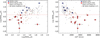Fig. 7 Rest-frame EW of [OIII]λ5007 as a functionof REWCIV (left) and $v_{\text{CIV}}^{\text{peak}}$ (right) for the WISSH targets with blue stars for the [OIII] sample and red stars for the Weak [OIII] sample, compared to the samples of Shen (2016), Tang et al. (2012), and Sulentic et al. (2017, and reference therein). The dashed red line refers to the WISSH [OIII] dichotomy, with REW[OIII] boundary value of 5 Å.

Fig. 8 FWHMCIV of the entire emission line profile as a function of $v_{\text{CIV}}^{\text{peak}}$ for the WISSH sample, compared to PG QSOs from Baskin & Laor (2005) and Tang et al. (2012; green diamonds), WLQs from Plotkin et al. (2015; orange circles), SDSS QSOs from Shen (2016) and Coatman et al. (2016: magenta squares and purple triangles respectively), and HE QSOs from Sulentic et al. (2017; top) and FWHM(CIV) of the outflow component (bottom) as a function of$v_{\text{CIV}}^{\text{peak}}$ for the WISSH sample. The black solid line indicates the best linear fits to the data and the purple dashed lines correspond to the 68% confidence interval.

Fig. 9 $FWH{M}_{\text{\_H}\beta }^{\text{BLR}}$ as a functionof $v_{\text{CIV}}^{\text{peak}}$ for the WISSH sample, compared to PG QSOs from Baskin & Laor (2005) and Tang et al. (2012; green diamonds), WLQs from Plotkin et al. (2015; orange circles), SDSS QSOs from Shen (2016) and Coatman et al. (2016; magenta squares and purple triangles, respectively), and HE QSOs from Sulentic et al. (2017).

4.3.2 Mass and kinetic power of CIV winds

We estimated the ionized gas mass (M_ion) of the outflow associated with the outflow component of the CIV emission line for the Weak [OIII] sources according to the following formula from Marziani et al. (2016). This relation assumes a constant density scenario for the CIV emitting gas (i.e. n(C³⁺)/n(C) = 1) and takes into account the carbon abundance: $$M_{\text{ion}}=9.5\times {10}^2\times L_{45}(CIV)\times Z_5^{-1}\times n_9^{-1}(M_{\odot }),$$(3)

where L₄₅(CIV) is the luminosity of the outflow component in units of 10⁴⁵ erg s⁻¹, Z₅ is the metallicity in units of 5 Z_⊙ (i.e. the typical value measured for the BLR in high-z luminous QSOs, Nagao et al. 2006), and n₉ is the gas density in units of 10⁹ cm⁻³. For the Weak [OIII] sample we estimated M_ion = 150–1100 M_⊙, assuming Z = 5 Z_⊙ and n = 10^9.5 cm⁻³ (see Table 8). From Eq. (3) it is possible to derive the mass outflow rate (Ṁ_ion), that is, the mass of ionized gas passing through a sphere of radius R, as $${\dot{M}}_{\text{ion}}=3\times (M_{\text{ion}}\times v)/R_1(M_{\odot }{\text{yr}}^{-1}),$$(4)

where v = $v_{\text{CIV}}^{\text{out}}$ and R₁ is the outflow radius in units of 1 pc. The BLR radius-luminosity relation (R_BLR ∝ $L_{5100}^{0.5}$, e.g., Bentz et al. 2009) indicates a typical radius of ~1 pc for the WISSH QSOs with luminosity L₅₁₀₀ > 6 × 10⁴⁶ erg s⁻¹. We inferred Ṁ_ion in the range ≈3–30 M_⊙ yr⁻¹, which is similar to the accretion rate for a quasar with L_Bol corresponding to the median L_Bol of the WISSH range, ~70 M_⊙ yr⁻¹ for L_Bol = 4 × 10⁴⁷ erg s⁻¹, assuming a radiative efficiency of 10%. Accordingly, the kinetic power of the outflow can be expressed as $${\dot{E}}_{\text{kin}}=\frac{1}{2}{\dot{M}}_{\text{ion}}\times v^2(\text{erg}{s}^{-1}).$$(5)

The resulting values of Ė_kin associated with the outflow component as a function of L_Bol are plotted in Fig. 10 as red filled symbols for objects in the Weak [OIII] sample.

Since the [OIII] QSOs also show an outflow component of the CIV emission (see Fig. 2), we were able to provide an estimate of Ṁ_ion, Ṁ_ion, and Ė_kin also for them. Moreover, as discussed in Sect. 4.1, [OIII] QSOs are supposed to be viewed at high inclination. Accordingly, we estimated Ṁ_ion and Ė_kin by assuming the so-called maximum velocity $v_{\text{CIV}}^{\text{max}}$ = $v_{\text{CIV}}^{\text{out}}$ + 2 $\times {\sigma }_{\text{CIV}}{}^{\text{out}}$, where ${\sigma }_{\text{CIV}}^{\text{out}}$ is the velocity dispersion of the outflow component, taking into account projection effects, and can be indeed considered representative of the bulk velocity of the outflow in the case of biconically symmetric outflowing gas (see Paper I and references therein). In Fig. 10the Ė_kin values associated with the outflow component in [OIII] sources are plotted as blue filled stars.

As mentioned in Sect. 4.3, the bulk of the virialized component of the CIV emission line is located bluewards 1549 Å in our fits for both the Weak [OIII] and (even slightly) [OIII] QSOs. This means that it can be also associated with an outflow and, therefore, we also derived M_ion, Ṁ_ion, and Ė_kin using Eqs. (3)–(5), considering its luminosity in addition to that of the outflow component and adopting $v_{\text{CIV}}^{\text{peak}}$ in the calculations of the outflow rates (see Table 9). The kinetic power derived by considering the entire profile of the CIV emission line are shown in Fig. 10 as red and blue empty symbols for the Weak [OIII] and [OIII] samples, respectively. In the case of Weak [OIII] sources, they are a factor of ≈2–10 smaller than the values based only on the luminosity and velocity of the outflow component ($v_{\text{CIV}}^{\text{peak}}$ < $v_{\text{CIV}}^{\text{out}}$), due to the Ė_kin ∝ v³ dependence. In the case of [OIII] sources, the Ė_kin calculated in this way are a factor of ≥100–1000 smaller than those derived by using $v_{\text{CIV}}^{\text{max}}$. Accordingly, they can be considered as very conservative estimates of Ė_kin.

As shown in Fig. 10, the bulk of the kinetic power of the BLR winds discovered in WISSH QSOs is Ė_kin ~ 10⁻⁵ × L_Bol for both Weak [OIII] and [OIII] QSOs. It is instructive to compare these Ė_kin with those inferred for ionized NLR winds traced by [OIII]. About 20% of the BLR winds detected in WISSH QSOs show kinetic powers comparable (i.e. 10⁻³ < Ė_kin/L_Bol < 10⁻²) to those estimated for NLR winds in [OIII] sources. Remarkably, in one case, J1538+0855, the outflows associated with CIV and [OIII] have consistent Ė_kin values (see Appendix A). This would suggest that we are possibly revealing the same outflow in two different gas phases at increasing distance from the AGN (in an energy conserving scenario). This further supports the idea that this object represents a hybrid showing a mixture of the distinctive properties of the two populations of Weak [OIII] and [OIII] QSOs.

Hereafter, we consider the outflow parameters derived by using $v_{\text{CIV}}^{\text{out}}$ and $v_{\text{CIV}}^{\text{max}}$ for the Weak [OIII]and the [OIII] QSOs, respectively, as the most representative ones. Figure 11 (left panel) shows a comparison of Ė_kin as a function of L_Bol between the NLR and BLR winds revealed in WISSH QSOs and a large collection of [OIII]-based NLR winds from a heterogeneous AGN sample reported in Fiore et al. (2017). A sizable fraction of BLR winds in Weak [OIII] and [OIII] QSOs are as powerful as NLR winds in less luminous QSOs, with Ė_kin < 10⁴³⁻⁴⁴ erg s⁻¹. This suggests that BLR winds should be taken into account to obtain a complete census of strong AGN-driven winds and comprehensively evaluate their effects of depositing energy and momentum into the ISM.

In order to give an idea of the possible uncertainties affecting the calculations of Ė_kin, in Fig. 11 (left panel) we show the maximum and minimum values obtained by considering a very large range of variation for the two fundamental parameters n_e and Z. More specifically, the lower bound corresponds to the assumption of n_e = 10¹⁰ cm⁻³ based on the presence of the semiforbidden line [CIII]λ1909 Å (Ferland & Elitzur 1984) and Z = 8 Z_⊙ (Nagao et al. 2006), while the upper bound corresponds to the assumption of n_e = 10⁹ cm⁻³, based on the absence of forbidden lines such as [OIII]λ4363 Å (Ferland & Elitzur 1984) and Z = 3 Z_⊙ (Nagao et al. 2006).

Figure 11 (right panel) displays the outflow momentum load (i.e. the ouflow momentum rate Ṗ_out (≡ Ṁ_out × v_out) normalized to the AGN radiation momentum rate Ṗ_AGN ≡ L_Bol /c) as a function of outflow velocity for different classes of outflow derived by Fiore et al. (2017), compared to those measured for the winds traced by the blueshifted CIV emission line in WISSH. The BLR winds in WISSH show velocities between those measured for X-ray ultra-fast (v > 10⁴ km s⁻¹) outflows (UFOs, crosses) and [OIII]-based outflows (v < 2000 km s⁻¹, triangles). This matches well with interpreting the outflow velocity distribution as a proxy of the distribution in radial distance from the AGN, that is, from the innermost region of the accretion disk (tens of gravitational radii for the UFOs; for example see Nardini et al. 2015; Tombesi et al. 2012, 2013; Gofford et al. 2015) up to kpc-scale in the case of the [OIII] winds (e.g., Harrison et al. 2012; Carniani et al. 2015; Cresci et al. 2015; Paper I).

The BLR winds typically exhibit a low momentum load, Ṗ_out/Ṗ_AGN <~ 0.1, which is a range poorly sampled by other ionized winds. Furthermore, the BLR winds seem to represent the low-power, low-velocity analogs of UFOs. The latter show Ṗ_out/Ṗ_AGN ~ 1, as expected in the case of quasi-spherical winds with electron scattering optical depth τ ~ 1 produced by systems accreting at λ_Edd ~ 1 (e.g. King 2010). UFOs are found to have a large covering factor (Nardini et al. 2015; King & Pounds 2015). BLR clouds in luminous AGN are expected to have a covering factor of ~0.1 (Netzer 1990). We can thus speculate that the low Ṗ_out∕Ṗ_AGN of BLR winds with respect to that of UFOs may be due to both a lower N_H and a lower covering factor of the CIV outflowing gas with respect to the fast, highly ionized gas responsible for the UFOs.

Fig. 10 Kinetic power of the BLR winds as a function of LBol. Red filled stars refer to values of Ėkin of the Weak [OIII] QSOs derived from the CIV outflow component using $v_{\text{CIV}}^{\text{out}}$. Blue filled stars refer to values of Ėkin of the [OIII] QSOs derived from the entire CIV profile using $v_{\text{CIV}}^{\text{max}}$. Blue and redempty stars refer to values of Ėkin derived from the entire CIV profile using $v_{\text{CIV}}^{\text{peak}}$, for the [OIII] and Weak [OIII] QSOs, respectively. BLR winds are compared with WISSH NLR ionized outflows from Paper I (green diamonds).

Fig. 11 Left panel: Kinetic power of the CIV outflow component as a function of LBol for the WISSH QSOs (red and blue stars) compared with WISSH NLR ionized outflows from Paper I (green diamonds) and other samples from literature, (e.g., Fiore et al. 2017 for details; purple triangles). The error bar (bottom right corner) is calculated as described in Sect. 4.3.2. Right panel: Wind momentum load as a function of the outflow velocity. The BLR winds traced by the CIV outflow components from the WISSH QSOs (red and blue stars) are compared with X-ray winds (magenta crosses) and ionized winds (green triangle). X-ray winds for Markarian 231 and IRASF11119+13257 are represented with a magenta diamond and circle, respectively.

5 What is the physical driver of the CIV velocity shift?

In order to shed light on the main physical driver of the large blueshifts of the CIV emission line observed in QSOs, we investigated the dependence of the CIV velocity shift on fundamental AGN parameters such as L_Bol, λ_Edd, and the UV-to-X-ray continuum slope (α_OX). Previous studies indeed found that $v_{\text{CIV}}^{\text{peak}}$ is correlated with all these three quantities (Marziani et al. 2016, Richards et al. 2011), but it still unclear which is thefundamental dependency. We proceeded as follows: we initially identified the main driver of $v_{\text{CIV}}^{\text{peak}}$ between L_Bol and λ_Edd and then we studied the dependency of $v_{\text{CIV}}^{\text{peak}}$ on this parameter and on α_OX.

5.1 Velocity shifts versus L_Bol and λ_Edd

We compared the WISSH sample to QSOs for which the BH mass and Eddington ratio are derived from the Hβ emission line, the “Hβ sample”, because of the large uncertainties of BH mass estimation from the CIV emission line, affected by the non-virialized component. All these sources therefore have reliable SMBH masses and λ_Edd.

Figure 12 shows $v_{\text{CIV}}^{\text{peak}}$ as a function ofL_Bol (left panel, a) and λ_Edd (right panel, b) for the WISSH and the “Hβ sample” QSOs. The blueshifts are clearly correlated with both L_Bol and λ_Edd. Specifically, we found a stronger correlation with L_Bol (Spearman rank r = 0.43 and P-value = 1.8 × 10⁻⁹) than with λ_Edd (Spearman rank r = 0.33 and P-value = 7.1 × 10⁻⁶), bearing in mind the large scatter affecting both relations.

Moreover, performing a least-squares regression, we found that 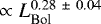$v_{\text{CIV}}^{\text{peak}}$ $\propto L_{\text{Bol}}^{0.28 \pm 0.04}$. This is consistent with a radiation-driven wind scenario (Laor & Brandt 2002), for which we indeed expect a terminal outflow velocity v_t $\propto \sqrt{L/R_{\ge BLR}}\propto L^{0.25}$ (valid for R ≥ R_BLR, e.g., Netzer & Laor 1993; Kaspi et al. 2000; Bentz et al. 2009). A similar dependence is also found for $v_{\text{CIV}}^{\text{peak}}$ as a function of M_BH. This lends further support to the radiative wind scenario and suggests that the radiation pressure is dominant over the Keplerian velocity field (for which a dependence of $\propto M_{\text{BH}}^{0.5}$ is expected).

In order to determine which is the fundamental variable between L_Bol and λ_Edd, we studied correlations between the residuals from (i) λ_Edd–L_Bol and $v_{\text{CIV}}^{\text{peak}}$–L_Bol relations, and (ii) L_Bol–λ_Edd and $v_{\text{CIV}}^{\text{peak}}$–λ_Edd relations (see Appendix B in Bernardi et al. 2005 for further details about residuals analysis). More specifically, we tested the hypothesis that the bolometric luminosity is the fundamental variable. In this case we expect: (i) no significant correlation between the residuals obtained from the λ_Edd–L_Bol (Δ_λ,L) and $v_{\text{CIV}}^{\text{peak}}$–L_Bol (Δ_{v, L}) relations; (ii) a correlation between residuals obtained from L_Bol–λ_Edd (Δ_L,λ) and $v_{\text{CIV}}^{\text{peak}}$–λ_Edd (Δ_v,λ) relations; (iii) that the slope of this correlation should be the same as the $v_{\text{CIV}}^{\text{peak}}$–L_Bol relation. The Δ_λ,L–Δ_{v, L} residuals are plotted in Fig. 12c. In this case we derived a Spearman rank r = 0.11 and P-value = 0.16, which indicates no correlation between parameters as expected from (i). In Fig. 12d the Δ_L,λ and Δ_v,λ residuals are plotted. In this case we found a strong correlation with a Spearman rank r = 0.32 and P-value = 1.1 × 10⁻⁵, with a slope consistent (2σ) with what we measured for the $v_{\text{CIV}}^{\text{peak}}$–L_Bol relation. We also created 1000 bootstrap samples from the residuals shown in Fig. 12d and calculated the corresponding Spearman rank, r. From the original residuals we derived r = 0.33 with a 95% confidence interval of 0.18–0.46, which is defined as the interval spanning the 2.5th to the 97.5th percentile of the resampled values. By combining these results, we conclude that L_Bol is the fundamental variable with respect to the λ_Edd and it can be considered as the main driver of the observed CIV blueshifts with respect to λ_Edd.

Fig. 12 The velocity shift $v_{\text{CIV}}^{\text{peak}}$ as a function of LBol (a) and as a function of λEdd (b), for the WISSH sample (blue and red stars) compared to the PG QSOs from Baskin & Laor (2005) and Tang et al. (2012; greendiamonds), WLQs from Plotkin et al. (2015; orange circles), SDSS QSOs from Shen (2016) and Coatman et al. (2016;magenta squares and purple triangles), and HE QSOs from Sulentic et al. (2017, and reference therein). The LBol for the HE sample has been derived from L5100 applying a bolometric correction of 5.6, as suggested by Runnoe et al. (2012) for the luminosity range of the HE sample. c) Residuals plot of λEdd–LBol and $v_{\text{CIV}}^{\text{peak}}$–LBol relations. d) Residuals plot of LBol–λEdd and $v_{\text{CIV}}^{\text{peak}}$–λEdd relations. The black lines indicate the best linear fits to the data and the purple lines correspond to the 68% confidence interval.

5.2 Velocity shifts versus L_Bol and α_OX

We performed the same analysis described in Sect. 5.1 considering L_Bol and α_OX, to investigate the primary driver of the CIV blueshifts. Figure 13 shows the $v_{\text{CIV}}^{\text{peak}}$ as a function of L_Bol and α_OX for 14 WISSH QSOs with both Hβ and X-ray measurements. For the WISSH QSOs, the α_OX was derived using the monochromatic luminosities at 2500 Å obtained from broadband SED fitting and the absorption-corrected luminosities at 2 keV (Martocchia et al. 2017). We compare our findings with those derived for 170 radio-quiet, broad-line QSOs from the Wu et al. (2009) sample and 29 WLQs (Luo et al. 2015; Wu et al. 2011) with available UV and X-ray information.

By performing a least-square fit also for this large sample, we confirm the results reported in Sect. 5.1 about the presence of a correlation between $v_{\text{CIV}}^{\text{peak}}$ and L_Bol, deriving a dependence $v_{\text{CIV}}^{\text{peak}}$ ∝ L_Bol ^{0.25 ± 0.06} (Spearman rank r = 0.30 and P-value = 1.1 × 10⁻⁵; see Fig. 13a). We found a very strong anti-correlation between the $v_{\text{CIV}}^{\text{peak}}$ and α_OX (Fig. 13b), that is, $v_{\text{CIV}}^{\text{peak}}$ ∝ α_OX ^{−1.07 ± 0.16} (Spearman rank r = –0.46 and P-value = 8.7 × 10⁻¹³), confirming the results reported in Richards et al. (2011).

We also performed the correlations analysis between the residuals from (i) $v_{\text{CIV}}^{\text{peak}}$–L_Bol (Δ_v,L) and α_OX–L_Bol (Δ_αox,L) relations, and (ii) $v_{\text{CIV}}^{\text{peak}}$–α_ox (Δ_v,αox) and L_Bol–α_ox (Δ_L,αox) relations, based on the hypothesis that L_Bol is the fundamental parameter. However, the results reported in Fig. 13c,d are at odds with this hypothesis, indicating a clear anti-correlation between Δ_{v, L} and Δ_{αox, L}, and no correlation between Δ_v,αox and Δ_L,αox. Furthermore, the slope of the residuals Δ_{v, L}-Δ_{αox, L} is consistent with that found for the α_OX–$v_{\text{CIV}}^{\text{peak}}$ relation. From a statistical point of view, this points to α_OX as the primary driver of the blueshifts of the CIV emission line observed in these QSOs.

We note that there is a well-known strong anti-correlation between α_OX and the UV luminosity (~L_Bol for Type I QSOs; e.g., Vignali et al. 2003; Steffen et al. 2006; Lusso et al. 2010; Martocchia et al. 2017) according to which the steeper the α_OX, the higher the luminosity. Therefore, both selecting steep α_OX or high L_Bol allows us to pick up fast outflows. We can conclude that the strength and the slope of the ionizing continuum is the main driver of the BLR winds. In Table 10 a summary of correlations of the CIV velocity shifts with physical quantities such as L_Bol, λ_Edd, M_BH and α_OX is reported. Results from residuals correlations are also listed.

The dependence of the velocity shift on both L_Bol and α_OX is in agreement with our scenario of radiation-driven wind, according to which a strong UV continuum is necessary tolaunch the wind but the level of extreme UV (EUV) and X-ray emission (i.e., up to 2 keV) is crucial to determine its existence, since strong X-ray radiation can easily overionize the gas and hamper an efficient line-driving mechanism. On the contrary, an X-ray weaker emission with respect to the optical-UV accretion disk emission can allow UV line opacity (Leighly 2004; Richards et al. 2011). Furthermore, as suggested by Wu et al. (2009), the increasing steepness of the α_OX (i.e., the softening of EUV–X-ray emission) at progressively higher UV luminosities may also explain the weakness of the CIV emission line (ionization potential 64.45 eV) in luminous QSOs; the strength of the line indeed depends on the number of the photons available to produce it, whereby a deficit of such ionizing photons leads to CIV weaker emission lines, as typically observed in Weak [OIII]QSOs and WLQs.

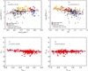Fig. 13 The velocity shift $v_{\text{CIV}}^{\text{peak}}$ as a function of LBol (a) and αOX (b), for the WISSH sample (blue and red stars) compared to radio quiet type-1 QSOs from Wu et al. (2009; black circles) and WLQs from Wu et al. (2011) and Luo et al. (2015; orange circles). c) Residuals plot of $v_{\text{CIV}}^{\text{peak}}$–LBol and αOX –LBol relations. d) Residuals plot of $v_{\text{CIV}}^{\text{peak}}$–αOX and LBol –αOX relations. The black lines represent the best linear fits to the data and the purple lines correspond to the 68% confidence interval.

6 Summary and conclusions

We have presented the results from the analysis of thirteen sources in the WISSH quasar sample with NIR spectroscopy from LBT/LUCI or VLT/SINFONI observations, in addition to five sources discussed in Paper I. We stress that these objects have been selected on the basis of a redshift for which the LBT/LUCI spectrum covers the [OIII] wavelength range and, therefore, can be considered as randomly selected from the entire WISSH QSOs sample. Our analysis has been performed with the goal of deriving the properties of (i) Hβ and [OIII] emission lines from the optical rest-frame spectra, and (ii) the CIV emission line by using rest-frame UV SDSS spectra. Our main findings can be summarized as follows:

• All the 18 WISSH QSOs considered here exhibit SMBHs with mass larger than 10⁹ M_⊙, with 50% of them hosting very massive SMBHs with M_BH >~ 5× 10⁹ M_⊙. Based on these Hβ-based M_BH values, we derived Eddington ratios 0.4 < λ_Edd < 3.1. This supports the evidence that the WISSH QSOs are powered by highly accreting SMBHs at the massive end of the SMBH mass function.

• According to the REW_[OIII] ≥ or < 5 Å, the WISSH QSOs can be divided into two samples: [OIII] and Weak [OIII] samples, respectively. In particular, six sources exhibit REW_[OIII] ≈ 7–70 Å, showing [OIII] profiles dominated by a broad blueshifted component, and 11 sources have REW_[OIII] ≈ 0.3–3 Å.

• As reported in Sect. 4.1, there is more than one explanation to ascribe to the WISSH REW_[OIII] distribution. One is in terms of orientation effect, with the [OIII] sample likely being seen at high (≈25–73 deg) inclination. This leads to a lower continuum luminosity and, hence, high REW_[OIII] values. On the contrary, the Weak [OIII] sources (including J1422+4417, see Sect. 3.1) are likely associated with nearly face-on AGNs. However, the weak [OIII] emission for the WISSH QSOs is expected to be due to the high bolometric luminosities of these sources. Indeed the [OIII] emission tends to decrease because of the over-ionization from the central engine, as found by Shen & Ho (2014). A further explanation for the difference in REW_[OIII] between the [OIII] and Weak [OIII] may be ascribed to the presence of a kpc-scale ionization cone oriented along the galaxy disk for the [OIII] objects, leading to a larger amount of gas to be ionized, while an ionization cone oriented perpendicular to the galaxy disk in the case of Weak [OIII] sample leads to a lower content of [OIII] gas to be ionized.

• Most of the WISSH QSOs exhibits 10 <~ REW_CIV <~ 20 Å with the peak of the CIV emission line profile blueshifted with respect to the systemic redshift ($v_{\text{CIV}}^{\text{peak}}$ ~ 2000–8000 km s⁻¹), indicating that the emitting gas is outflowing. This suggests that the luminosity-based selection criterion of WISSH is very effective in collecting strong CIV winds. Historically, such large CIV blueshifts have been associated with fainter CIV emitting QSOs, that is, the WLQs (Plotkin et al. 2015), although very recently Hamann et al. (2017) have reported the existence of ERQs showing CIV winds and extremely large REW_CIV (i.e., > 100 Å). We found that QSOs belonging to the Weak [OIII] sample, representing 70% of the WISSH sample analyzed here, show a broad asymmetric blueward and relatively weak (i.e., REW_CIV < 20 Å) CIV line profile (see Fig. 7), with the peak of the entire CIV profile extremely blueshifted ($v_{\text{CIV}}^{\text{peak}}$ ≥ 2000 km s⁻¹ up to 8000 km s⁻¹). On the contrary, 30% of the WISSH QSOs (i.e., [OIII] sample) have a peaked CIV profile with REW_CIV > 20 Å and $v_{\text{CIV}}^{\text{peak}}$ ≤ 2000 km s⁻¹. High-luminosity, optically-selected HE QSOs from Sulentic et al. (2017) follow a similar trend by populating the same region of the WISSH QSOs in the plane REW_CIV-$v_{\text{CIV}}^{\text{peak}}$ as shown in Fig. 6 and REW_[OIII]–$v_{\text{CIV}}^{\text{peak}}$ in Fig. 7.

This highlights a dichotomy in the detection of NLR and BLR winds in WISSH QSOs, which could be likely due to inclination effects in a polar geometry scenario for the CIV winds, as suggested in Sect. 4.3.

We found that a sizable fraction of WISSH QSOs exhibit BLR winds traced by CIV blueshifted emission with Ṁ_ion ≈ 10–100 M_⊙ yr⁻¹, comparable with the median accretion rate of WISSH QSOs. Twenty percent of the BLR winds detected in WISSH QSOs show kinetic powers 10⁻³ < Ė_kin/L_Bol < 10⁻², which is comparable to those measured for NLR winds associated with [OIII] broad or blueshifted emission lines detected in the [OIII] sample. The remaining 80% of the BLR winds show kinetic powers comparable to those traced by [OIII] in less luminous AGNs. This suggests that the BLR winds should be taken into account to obtain a complete census of strong AGN-driven outflows and comprehensively evaluate their effects of depositing energy and momentum into the ISM.

The BLR winds traced by the CIV emission line exhibit a velocity range (v${}_{\text{CIV}}^{\text{out/max}}$ ≈ 2000–13 000 km s⁻¹) between those measured for UFO (at sub-pc scale) and NLR winds (at kpc-scale), interpreting the outflow velocity distribution as a proxy of the distribution in radial distance for different classes of outflows (see Fig. 11). Moreover, the BLR winds exhibit a Ṗ_out/Ṗ_AGN <~ 0.1, which is lower than that found for UFOs (i.e., Ṗ_out/Ṗ_AGN ~ 1). In this case the momentum rate of the outflow is comparable to that of the AGN, suggesting a covering factor for the UFOs of the order of unity. Since the covering factor for the BLR is expected to be ~0.1, we can thus speculate that the momentum load of the nuclear winds may reflect the covering factor of the outflowing gas.

We investigated the dependence of $v_{\text{CIV}}^{\text{peak}}$ on fundamentalAGN physical parameters such as L_Bol, λ_Edd, and α_OX. We found a stronger correlation with L_Bol than λ_Edd (see Fig. 12), with a dependence consistent with a radiatively-driven winds scenario ($v_{\text{CIV}}^{\text{peak}}$ ∝ L_Bol ^{0.28 ± 0.04}). Moreover, we further studied the dependence of $v_{\text{CIV}}^{\text{peak}}$ on α_OX, finding a stronger correlation with α_OX than L_Bol. This relation is expected due to the dependence of α_OX on L_Bol (Vignali et al. 2003), that is, when α_OX is steeper, L_Bol is larger. This indicates that the shape of the ionizing continuum could be considered as the primary driver of the blueshifts of the CIV emission line.

Acknowledgements

We thank the anonymous referee for helpful comments that improved the paper. We acknowledge very useful discussions with P. Marziani, B. Husemann and D. Kakkad. We thank M. Vestergaard for kindly providing the UV FeII templates. The scientific results reported in this article are based on observations made by the LBT, the European Southern Observatory (ESO program 093.A–0175(A. B)), and the SDSS. The LBT is an international collaboration among institutions in the United States, Italy, and Germany. LBT Corporation partners are: The University of Arizona on behalf of the Arizona Board of Regents; Istituto Nazionale di Astrofisica, Italy; LBT Beteiligungsgesellschaft, Germany, representing the Max-Planck Society, the Astrophysical Institute Potsdam, and Heidelberg University; The Ohio State University, and The Research Corporation, on behalf of The University of Notre Dame, University of Minnesota and University of Virginia. Funding for the Sloan Digital Sky Survey IV has been provided by the Alfred P. Sloan Foundation, the U.S. Department of Energy Office of Science, and the Participating Institutions. SDSS acknowledges support and resources from the Center for High-Performance Computing at the University of Utah. The SDSS web site is https://www.sdss.org/. The SDSS is managed by the Astrophysical Research Consortium for the Participating Institutions. The Participating Institutions are the American Museum of Natural History, Astrophysical Institute Potsdam, University of Basel, University of Cambridge, Case Western Reserve University, University of Chicago, Drexel University, Fermilab, the Institute for Advanced Study, the Japan Participation Group, Johns Hopkins University, the Joint Institute for Nuclear Astrophysics, the Kavli Institute for Particle Astrophysics and Cosmology, the Korean Scientist Group, the Chinese Academy of Sciences (LAMOST), Los Alamos National Laboratory, the Max-Planck-Institute for Astronomy (MPIA), the Max-Planck-Institute for Astrophysics (MPA), New Mexico State University, Ohio State University, University of Pittsburgh, University of Portsmouth, Princeton University, the United States Naval Observatory, and the University of Washington. This research has made use of the NASA/IPAC Extragalactic Database (NED), which is operated by the Jet Propulsion Laboratory, California Institute of Technology, under contract with the National Aeronautics and Space Administration. This research project was supported by the DFG Cluster of Excellence “Origin and Structure of the Universe” (www.universe-cluster.de). We acknowledge financial support from PRIN-INAF 2014 (Windy Black Holes combing galaxy evolution). A. Bongiorno and E. Piconcelli acknowledge financial support from INAF under the contract PRIN-INAF-2012. L. Zappacosta acknowledges financial support under ASI/INAF contract I/037/12/0. G. Bruni acknowledges financial support under the INTEGRAL ASI-INAF agreement 2013-025.R01. F. Tombesi acknowledges support from the 2014 MIUR grant “Rita Levi Montalcini”. S. Bisogni is supported by the National Aeronautics and Space Administration through Chandra Award Number AR7–18013 X issued by the Chandra X-ray Observatory Center, which is operated by the Smithsonian Astrophysical Observatory for and on behalf of the National Aeronautics Space Administration under contract NAS8–03060. We are grateful to M. Fumana for his assistance in LBT data reduction.

Appendix A SDSS J1538+0855

We present here a detailed analysis of the source J1538+0855 since it is the only object exhibiting both NLR and BLR winds. As reported in Sect. 4.3.2, we measured the CIV outflow properties based on the so-called outflow component. We estimated the gas mass of the outflow as M_ion = 590 M_⊙, the maximum velocity of the outflow as representative of the bulk velocity of the outflow, $v_{\text{CIV}}^{\text{max}}$ = 13 400 km s⁻¹, the ionized gas mass rate asṀ_ion = 24 M_⊙ yr⁻¹, and the kinetic power as Ė_kin = 1.4 × 10⁴⁵ erg s⁻¹. We also measured the properties of the CIV outflow considering the entire CIV profile, with the $v_{\text{CIV}}^{\text{peak}}$ as representative of the outflow velocity. We estimated M_ion = 1210 M_⊙, a ionized gas mass rate Ṁ_ion = 8 M_⊙ yr ⁻¹, and a kinetic power Ė_kin = 12 × 10⁴² erg s⁻¹.

As mentioned in Sect. 3, we found a broad (~2000 km s⁻¹), blueshifted (4987 Å) [OIII] component, indicative of outflow. In order to characterize the ionized outflowing gas, we calculated the mass rate Ṁ and the kinetic power Ė_kin, assuming the outflow model discussed in Paper I and using the [OIII] emission line. According to Equations (2), (5), and (6) in Paper I, we derived $M_{\text{ion}}^{[\text{OIII}]}$ = 4.2 × 10⁸ M_⊙, ${\dot{M}}_{\text{ion}}^{[\text{OIII}]}$ = 530 M_⊙ yr⁻¹, and ${\dot{E}}_{\text{kin}}^{[\text{OIII}]}$ = 1.4 × 10⁴⁵ erg s⁻¹ of the ionized outflow, assuming an electron density of n_e = 200 cm⁻³, a solar metallicity, and an outflow velocity defined as v_max = |Δv| + 2${\sigma }_{[\text{OIII}]}^{\text{broad}}$, where Δ v is the velocity shift between the broad [OIII] component and the systemic [OIII] assumed at 5007 Å, and ${\sigma }_{[\text{OIII}]}^{\text{broad}}$ is the velocity dispersion of the broad [OIII] component (v_max = 2900 km s⁻¹). We refer to Paper I for more details about the assumptions used in the calculation of the outflow parameters.

We investigated how the values of ${\dot{M}}_{\text{ion}}^{[\text{OIII}]}$ and ${\dot{E}}_{\text{kin}}^{[\text{OIII}]}$ are sensitiveto different assumed parameters. As in paper I, the upper bound corresponds to the assumption of n_e = 80 cm⁻³ (as in Genzel et al. 2014) and we determined that ${\dot{M}}_{\text{ion}}^{[\text{OIII}]}$ = 1330 M_⊙ yr⁻¹ and ${\dot{E}}_{\text{kin}}^{[\text{OIII}]}$ = 3.5 × 10⁴⁵ erg s⁻¹, while the lower bound corresponds to n_e = 1000 cm⁻³ (typical value for the NLR, Peterson 1997) and a velocity of W₈₀/1.3 (as in Harrison et al. 2014), where W₈₀ is the velocity width of the line at 80% of the line flux. We derived a lower bound of ${\dot{M}}_{\text{ion}}^{[\text{OIII}]}$ = 60 M_⊙ yr⁻¹ and ${\dot{E}}_{\text{kin}}^{[\text{OIII}]}$ = 5 × 10⁴³ erg s⁻¹.

Appendix B Optical rest-frame spectra of 13 WISSH QSOs

We present the LBT/LUCI and SINFONI optical rest-frame spectra in the wavelength range of the Hβ-[OIII] emission lines for the 13 WISSH QSOs analyzed in the present paper (see Table 1).

Fig. B.1 Thered line shows the best fit of the spectrum. Green curve refers to the core component associated with the NLR emission of Hβ and [OIII] emission lines. Blue curve refers to the broad blueshifted emission of [OIII]λλ4959,5007 Å, indicative of outflow. Gold curve indicates the broad component of Hβ associated with BLR emission. FeII emission is indicated in magenta. Grey band indicates the region excluded from the fit because of the presence of sky line residual. Lower panel shows the fit residuals.

Appendix C SDSS Optical/UV rest-frame spectra of 18 WISSH QSOs

We present the SDSS DR10 UV rest-frame spectra of the 18 WISSH QSOs analyzed in the present paper.

Fig. C.1 SDSS DR10 UV rest-frame spectra. The red line shows the best-fit of the spectrum. Green curve refers to the core component likely associated with the NLR emission of the CIV emission. Blue curve refers to the broad blueshifted emission of CIV emission line, indicative of outflow. Gold curve indicates the broad virialized component associated with the BLR emission. FeII emission is indicated in magenta. Grey bands indicate the region excluded from the fit because of the presence of absorption lines. The dashed line denotes the CIVλ1549 Å rest-frame wavelength. Lower panel shows the fit residuals.

Fig. C.2 Same legend as in Fig. C.1.

Fig. C.3 Same legend as in Fig. C.1.

Fig. C.4 Same legend as in Fig. C.1.

Fig. C.5 Same legend as in Fig. C.1.

Fig. C.6 Same legend as in Fig. C.1.

Fig. C.7 Same legend as in Fig. C.1.

Fig. C.8 Same legend as in Fig. C.1.

Fig. C.9 Same legend as in Fig. C.1.

Fig. C.10 Same legend as in Fig. C.1.

Fig. C.11 Same legend as in Fig. C.1.

Fig. C.12 Same legend as in Fig. C.1.

Fig. C.13 Same legend as in Fig. C.1.

Fig. C.14 Same legend as in Fig. C.1.

Fig. C.15 Same legend as in Fig. C.1.

Fig. C.16 Same legend as in Fig. C.1.

Fig. C.17 Same legend as in Fig. C.1.

Fig. C.18 Same legend as in Fig. C.1.

References

All Tables

All Figures

Fig. 1 Parametrization of the Hβ-[OIII] region of the WISSH QSO J0958+2827. The red line shows the best fit to the data. Green curve refers to the core component associated with the NLR emission of Hβ and [OIII] emission lines. The blue curve refers to the broad blueshifted emission of [OIII]λλ4959, 5007 Å, indicative of outflow (but see Sect. 3.1 for more details). Gold curve indicates the broad component of Hβ associated with BLR emission. FeII emission is marked in magenta.

In the text

Fig. 2 Parametrization of the CIV emission line profile of the Weak [OIII] quasar J1422+4417 (upper panel) and the [OIII] quasar J0745+4734 (lower panel). In both panels the red, yellow, and blue curves refer to the best fit of the spectrum, virialized component, and outflow component of the CIV emission line, respectively. The black dashed line indicates the λCIV at 1549 Å. The red dotted-dashed line denotes the peak of the CIV emission line and$v_{\text{CIV}}^{\text{peak}}$ represents its velocity shift with respect to the systemic λ1549 Å. The blue dotted-dashed line indicates the peak of the outflow component and $v_{\text{CIV}}^{\text{out}}$ is its velocity shift with respect to the systemic redshift. In the lower panel the green curve refers to an additional Gaussian component required by the fit, in order to better describe the CIV profile in this QSO.

In the text

	Fig. 3 Observed distribution of the WISSH QSOs for the [OIII] and Weak [OIII] samples of (a) REW[OIII] and (b) REWH β, compared to the best fit of the REW[OIII] and REWHβ observed distribution of SDSS DR7 AGNs of Bisogni et al. (2017a) (black solid line).
In the text

	Fig. 4 Average SEDs corresponding to WISE photometry of the WISSH [OIII] (dashed blue line) and Weak [OIII] samples (red line), normalized at 15 μm (dot-dashed line).
In the text

Fig. 5 Bolometric luminosity as a function of BH mass for the WISSH sample, compared to PG QSOs from Tang et al. (2012) and Baskin & Laor (2005), and WLQs from Plotkin et al. (2015). Luminosity in fractions of 0.1, 0.5, and 1 Eddingtonluminosity are respectively indicated with dot-dashed, dotted, and dashed lines. Contours levels (0.01, 0.1, 0.5, and 0.9 relative to the peak) refer to SDSS DR7 QSOs from Shen et al. (2011).

In the text

Fig. 6 REWCIV as a functionof $v_{\text{CIV}}^{\text{peak}}$ for different samples. The WISSH QSOs are indicated by blue and red stars, for the [OIII] and Weak [OIII] sample respectively.The BAL WISSH QSOs are indicated with black circles. Contours levels (0.03, 0.1, 0.5, and 0.9 relative to the peak) refer to the SDSS DR7 sample from Shen et al. (2011). The green diamonds indicate the PG QSOs from Baskin & Laor (2005) and Tang et al. (2012). The orange circles refer to the sample of WLQs from Plotkin et al. (2015), Luo et al. (2015), and Wu et al. (2011), the brown crosses indicate the HE QSOs from Sulentic et al. (2017), the ERQs from Hamann et al. (2017) are indicated with purple triangles. The purple dashed line marks the REWCIV = 10 Å, which is the threshold for the WLQs. The distribution of the REWCIV and $v_{\text{CIV}}^{\text{peak}}$ are on the right and on the bottom, respectively.

In the text

Fig. 7 Rest-frame EW of [OIII]λ5007 as a functionof REWCIV (left) and $v_{\text{CIV}}^{\text{peak}}$ (right) for the WISSH targets with blue stars for the [OIII] sample and red stars for the Weak [OIII] sample, compared to the samples of Shen (2016), Tang et al. (2012), and Sulentic et al. (2017, and reference therein). The dashed red line refers to the WISSH [OIII] dichotomy, with REW[OIII] boundary value of 5 Å.

In the text

Fig. 8 FWHMCIV of the entire emission line profile as a function of $v_{\text{CIV}}^{\text{peak}}$ for the WISSH sample, compared to PG QSOs from Baskin & Laor (2005) and Tang et al. (2012; green diamonds), WLQs from Plotkin et al. (2015; orange circles), SDSS QSOs from Shen (2016) and Coatman et al. (2016: magenta squares and purple triangles respectively), and HE QSOs from Sulentic et al. (2017; top) and FWHM(CIV) of the outflow component (bottom) as a function of$v_{\text{CIV}}^{\text{peak}}$ for the WISSH sample. The black solid line indicates the best linear fits to the data and the purple dashed lines correspond to the 68% confidence interval.

In the text

	Fig. 9 $FWH{M}_{\text{\_H}\beta }^{\text{BLR}}$ as a functionof $v_{\text{CIV}}^{\text{peak}}$ for the WISSH sample, compared to PG QSOs from Baskin & Laor (2005) and Tang et al. (2012; green diamonds), WLQs from Plotkin et al. (2015; orange circles), SDSS QSOs from Shen (2016) and Coatman et al. (2016; magenta squares and purple triangles, respectively), and HE QSOs from Sulentic et al. (2017).
In the text

Fig. 10 Kinetic power of the BLR winds as a function of LBol. Red filled stars refer to values of Ėkin of the Weak [OIII] QSOs derived from the CIV outflow component using $v_{\text{CIV}}^{\text{out}}$. Blue filled stars refer to values of Ėkin of the [OIII] QSOs derived from the entire CIV profile using $v_{\text{CIV}}^{\text{max}}$. Blue and redempty stars refer to values of Ėkin derived from the entire CIV profile using $v_{\text{CIV}}^{\text{peak}}$, for the [OIII] and Weak [OIII] QSOs, respectively. BLR winds are compared with WISSH NLR ionized outflows from Paper I (green diamonds).

In the text

Fig. 11 Left panel: Kinetic power of the CIV outflow component as a function of LBol for the WISSH QSOs (red and blue stars) compared with WISSH NLR ionized outflows from Paper I (green diamonds) and other samples from literature, (e.g., Fiore et al. 2017 for details; purple triangles). The error bar (bottom right corner) is calculated as described in Sect. 4.3.2. Right panel: Wind momentum load as a function of the outflow velocity. The BLR winds traced by the CIV outflow components from the WISSH QSOs (red and blue stars) are compared with X-ray winds (magenta crosses) and ionized winds (green triangle). X-ray winds for Markarian 231 and IRASF11119+13257 are represented with a magenta diamond and circle, respectively.

In the text

Fig. 12 The velocity shift $v_{\text{CIV}}^{\text{peak}}$ as a function of LBol (a) and as a function of λEdd (b), for the WISSH sample (blue and red stars) compared to the PG QSOs from Baskin & Laor (2005) and Tang et al. (2012; greendiamonds), WLQs from Plotkin et al. (2015; orange circles), SDSS QSOs from Shen (2016) and Coatman et al. (2016;magenta squares and purple triangles), and HE QSOs from Sulentic et al. (2017, and reference therein). The LBol for the HE sample has been derived from L5100 applying a bolometric correction of 5.6, as suggested by Runnoe et al. (2012) for the luminosity range of the HE sample. c) Residuals plot of λEdd–LBol and $v_{\text{CIV}}^{\text{peak}}$–LBol relations. d) Residuals plot of LBol–λEdd and $v_{\text{CIV}}^{\text{peak}}$–λEdd relations. The black lines indicate the best linear fits to the data and the purple lines correspond to the 68% confidence interval.

In the text

Fig. 13 The velocity shift $v_{\text{CIV}}^{\text{peak}}$ as a function of LBol (a) and αOX (b), for the WISSH sample (blue and red stars) compared to radio quiet type-1 QSOs from Wu et al. (2009; black circles) and WLQs from Wu et al. (2011) and Luo et al. (2015; orange circles). c) Residuals plot of $v_{\text{CIV}}^{\text{peak}}$–LBol and αOX –LBol relations. d) Residuals plot of $v_{\text{CIV}}^{\text{peak}}$–αOX and LBol –αOX relations. The black lines represent the best linear fits to the data and the purple lines correspond to the 68% confidence interval.

In the text

Fig. B.1 Thered line shows the best fit of the spectrum. Green curve refers to the core component associated with the NLR emission of Hβ and [OIII] emission lines. Blue curve refers to the broad blueshifted emission of [OIII]λλ4959,5007 Å, indicative of outflow. Gold curve indicates the broad component of Hβ associated with BLR emission. FeII emission is indicated in magenta. Grey band indicates the region excluded from the fit because of the presence of sky line residual. Lower panel shows the fit residuals.

In the text

Fig. C.1 SDSS DR10 UV rest-frame spectra. The red line shows the best-fit of the spectrum. Green curve refers to the core component likely associated with the NLR emission of the CIV emission. Blue curve refers to the broad blueshifted emission of CIV emission line, indicative of outflow. Gold curve indicates the broad virialized component associated with the BLR emission. FeII emission is indicated in magenta. Grey bands indicate the region excluded from the fit because of the presence of absorption lines. The dashed line denotes the CIVλ1549 Å rest-frame wavelength. Lower panel shows the fit residuals.

In the text

	Fig. C.2 Same legend as in Fig. C.1.
In the text

	Fig. C.3 Same legend as in Fig. C.1.
In the text

	Fig. C.4 Same legend as in Fig. C.1.
In the text

	Fig. C.5 Same legend as in Fig. C.1.
In the text

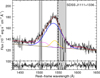	Fig. C.6 Same legend as in Fig. C.1.
In the text

	Fig. C.7 Same legend as in Fig. C.1.
In the text

	Fig. C.8 Same legend as in Fig. C.1.
In the text

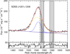	Fig. C.9 Same legend as in Fig. C.1.
In the text

	Fig. C.10 Same legend as in Fig. C.1.
In the text

	Fig. C.11 Same legend as in Fig. C.1.
In the text

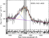	Fig. C.12 Same legend as in Fig. C.1.
In the text

	Fig. C.13 Same legend as in Fig. C.1.
In the text

	Fig. C.14 Same legend as in Fig. C.1.
In the text

	Fig. C.15 Same legend as in Fig. C.1.
In the text

	Fig. C.16 Same legend as in Fig. C.1.
In the text

	Fig. C.17 Same legend as in Fig. C.1.
In the text

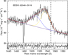	Fig. C.18 Same legend as in Fig. C.1.
In the text

References

- Ahn, C. P., Alexandroff, R., Allende Prieto, C., et al. 2014, ApJS, 211, 17 [NASA ADS] [CrossRef] [Google Scholar]
- Baskin, A., & Laor, A. 2005, MNRAS, 356, 1029 [NASA ADS] [CrossRef] [Google Scholar]
- Bentz, M. C., Peterson, B. M., Netzer, H., Pogge, R. W., & Vestergaard, M. 2009, ApJ, 697, 160 [Google Scholar]
- Bernardi, M., Sheth, R. K., Nichol, R. C., Schneider, D. P., & Brinkmann, J. 2005, AJ, 129, 61 [NASA ADS] [CrossRef] [Google Scholar]
- Bischetti, M., Piconcelli, E., Vietri, G., et al. 2017, A&A, 598, A122 [NASA ADS] [CrossRef] [EDP Sciences] [Google Scholar]
- Bisogni, S., Marconi, A., & Risaliti, G. 2017a, MNRAS, 464, 385 [NASA ADS] [CrossRef] [Google Scholar]
- Bisogni, S., Marconi, A., Risaliti, G., & Lusso, E. 2017b, Fr. Astron. Space Sci., 4, 48 [Google Scholar]
- Bongiorno, A., Maiolino, R., Brusa, M., et al. 2014, MNRAS, 443, 2077 [NASA ADS] [CrossRef] [Google Scholar]
- Boroson, T. A. 2002, ApJ, 565, 78 [NASA ADS] [CrossRef] [Google Scholar]
- Boroson, T. A., & Green, R. F. 1992, ApJS, 80, 109 [NASA ADS] [CrossRef] [Google Scholar]
- Bruni, G., Mack, K.-H., Salerno, E., et al. 2012, A&A, 542, A13 [NASA ADS] [CrossRef] [EDP Sciences] [Google Scholar]
- Brusa, M., Bongiorno, A., Cresci, G., et al. 2015, MNRAS, 446, 2394 [NASA ADS] [CrossRef] [Google Scholar]
- Cano-Díaz, M., Maiolino, R., Marconi, A., et al. 2012, A&A, 537, L8 [NASA ADS] [CrossRef] [EDP Sciences] [Google Scholar]
- Carniani, S., Marconi, A., Maiolino, R., et al. 2015, A&A, 580, A102 [NASA ADS] [CrossRef] [EDP Sciences] [Google Scholar]
- Cicone, C., Maiolino, R., Sturm, E., et al. 2014, A&A, 562, A21 [NASA ADS] [CrossRef] [EDP Sciences] [Google Scholar]
- Coatman, L., Hewett, P. C., Banerji, M., & Richards, G. T. 2016, MNRAS, 461, 647 [NASA ADS] [CrossRef] [Google Scholar]
- Coatman, L., Hewett, P. C., Banerji, M., et al. 2017, MNRAS, 465, 2120 [NASA ADS] [CrossRef] [Google Scholar]
- Corbin, M. R., & Boroson, T. A. 1996, ApJS, 107, 69 [NASA ADS] [CrossRef] [Google Scholar]
- Cresci, G., Mainieri, V., Brusa, M., et al. 2015, ApJ, 799, 82 [Google Scholar]
- Davies, R. I. 2007, MNRAS, 375, 1099 [NASA ADS] [CrossRef] [Google Scholar]
- Denney, K. D. 2012, ApJ, 759, 44 [NASA ADS] [CrossRef] [Google Scholar]
- Di Matteo, T., Springel, V., & Hernquist, L. 2005, Nature, 433, 604 [NASA ADS] [CrossRef] [PubMed] [Google Scholar]
- Diamond-Stanic, A. M., Fan, X., Brandt, W. N., et al. 2009, ApJ, 699, 782 [NASA ADS] [CrossRef] [Google Scholar]
- Duras, F., Bongiorno, A., Piconcelli, E., et al. 2017, A&A, 604, A67 [NASA ADS] [CrossRef] [EDP Sciences] [Google Scholar]
- Fabian, A. C. 2012, ARA&A, 50, 455 [NASA ADS] [CrossRef] [Google Scholar]
- Fan, X., Strauss, M. A., Gunn, J. E., et al. 1999, ApJ, 526, L57 [NASA ADS] [CrossRef] [PubMed] [Google Scholar]
- Faucher-Giguère, C.-A., & Quataert, E. 2012, MNRAS, 425, 605 [NASA ADS] [CrossRef] [Google Scholar]
- Ferland, G. J., & Elitzur, M. 1984, ApJ, 285, L11 [NASA ADS] [CrossRef] [Google Scholar]
- Ferland, G. J., Porter, R. L., van Hoof, P. A. M., et al. 2013, Rev. Mexicana Astron. Astrofis., 49, 137 [Google Scholar]
- Feruglio, C., Maiolino, R., Piconcelli, E., et al. 2010, A&A, 518, L155 [NASA ADS] [CrossRef] [EDP Sciences] [Google Scholar]
- Feruglio, C., Fiore, F., Carniani, S., et al. 2015, A&A, 583, A99 [NASA ADS] [CrossRef] [EDP Sciences] [Google Scholar]
- Fiore, F., Feruglio, C., Shankar, F., et al. 2017, A&A, 601, A143 [NASA ADS] [CrossRef] [EDP Sciences] [Google Scholar]
- Freudling, W., Romaniello, M., Bramich, D. M., et al. 2013, A&A, 559, A96 [NASA ADS] [CrossRef] [EDP Sciences] [Google Scholar]
- Gaskell, C. M. 1982, ApJ, 263, 79 [NASA ADS] [CrossRef] [Google Scholar]
- Genzel, R., Förster Schreiber, N. M., Rosario, D., et al. 2014, ApJ, 796, 7 [Google Scholar]
- Gofford, J., Reeves, J. N., Tombesi, F., et al. 2013, MNRAS, 430, 60 [Google Scholar]
- Gofford, J., Reeves, J. N., McLaughlin, D. E., et al. 2015, MNRAS, 451, 4169 [Google Scholar]
- Granato, G. L., De Zotti, G., Silva, L., Bressan, A., & Danese, L. 2004, ApJ, 600, 580 [Google Scholar]
- Gunn, J. E., Siegmund, W. A., Mannery, E. J., et al. 2006, AJ, 131, 2332 [NASA ADS] [CrossRef] [Google Scholar]
- Hall, P. B., Anderson, S. F., Strauss, M. A., et al. 2002, ApJS, 141, 267 [NASA ADS] [CrossRef] [Google Scholar]
- Hamann, F., Zakamska, N. L., Ross, N., et al. 2017, MNRAS, 464, 3431 [NASA ADS] [CrossRef] [Google Scholar]
- Harrison, C. M., Alexander, D. M., Swinbank, A. M., et al. 2012, MNRAS, 426, 1073 [NASA ADS] [CrossRef] [Google Scholar]
- Harrison, C. M., Alexander, D. M., Mullaney, J. R., & Swinbank, A. M. 2014, MNRAS, 441, 3306 [Google Scholar]
- Hewett, P. C.,& Wild, V. 2010, MNRAS, 405, 2302 [NASA ADS] [Google Scholar]
- Just, D. W., Brandt, W. N., Shemmer, O., et al. 2007, ApJ, 665, 1004 [Google Scholar]
- Kashi, A., Proga, D., Nagamine, K., Greene, J., & Barth, A. J. 2013, ApJ, 778, 50 [NASA ADS] [CrossRef] [Google Scholar]
- Kaspi, S., Smith, P. S., Netzer, H., et al. 2000, ApJ, 533, 631 [NASA ADS] [CrossRef] [Google Scholar]
- King, A., & Pounds, K. 2015, ARA&A, 53, 115 [Google Scholar]
- King, A. R. 2010, MNRAS, 402, 1516 [NASA ADS] [CrossRef] [Google Scholar]
- Kormendy, J., & Richstone, D. 1995, ARA&A, 33, 581 [NASA ADS] [CrossRef] [Google Scholar]
- Laor, A., & Brandt, W. N. 2002, ApJ, 569, 641 [NASA ADS] [CrossRef] [Google Scholar]
- Leighly, K. M. 2004, ApJ, 611, 125 [NASA ADS] [CrossRef] [Google Scholar]
- Luo, B., Brandt, W. N., Hall, P. B., et al. 2015, ApJ, 805, 122 [NASA ADS] [CrossRef] [Google Scholar]
- Lusso, E., Comastri, A., Vignali, C., et al. 2010, A&A, 512, A34 [NASA ADS] [CrossRef] [EDP Sciences] [Google Scholar]
- Markwardt, C. B. 2009, in Astronomical Data Analysis Software and Systems XVIII, eds. D. A. Bohlender, D. Durand, & P. Dowler, ASP Conf. Ser., 411, 251 [NASA ADS] [Google Scholar]
- Martocchia, S., Piconcelli, E., Zappacosta, L., et al. 2017, A&A, 608, A51 [NASA ADS] [CrossRef] [EDP Sciences] [Google Scholar]
- Marziani, P., Sulentic, J. W., Zwitter, T., Dultzin-Hacyan, D., & Calvani, M. 2001, ApJ, 558, 553 [NASA ADS] [CrossRef] [Google Scholar]
- Marziani, P., Sulentic, J. W., Stirpe, G. M., Zamfir, S., & Calvani, M. 2009, A&A, 495, 83 [NASA ADS] [CrossRef] [EDP Sciences] [Google Scholar]
- Marziani, P., Sulentic, J. W., Negrete, C. A., et al. 2010, MNRAS, 409, 1033 [NASA ADS] [CrossRef] [Google Scholar]
- Marziani, P., Martínez Carballo, M. A., Sulentic, J. W., et al. 2016, Ap&SS, 361, 29 [NASA ADS] [CrossRef] [Google Scholar]
- Matsuoka, K., Silverman, J. D., Schramm, M., et al. 2013, ApJ, 771, 64 [NASA ADS] [CrossRef] [Google Scholar]
- McGill, K. L., Woo, J.-H., Treu, T., & Malkan, M. A. 2008, ApJ, 673, 703 [NASA ADS] [CrossRef] [Google Scholar]
- Menci, N., Fiore, F., Puccetti, S., & Cavaliere, A. 2008, ApJ, 686, 219 [NASA ADS] [CrossRef] [Google Scholar]
- Nagao, T., Marconi, A., & Maiolino, R. 2006, A&A, 447, 157 [NASA ADS] [CrossRef] [EDP Sciences] [Google Scholar]
- Nardini, E., Reeves, J. N., Gofford, J., et al. 2015, Science, 347, 860 [Google Scholar]
- Netzer, H. 1990, in Active Galactic Nuclei, eds. R. D. Blandford, H. Netzer, L. Woltjer, T. J.-L. Courvoisier, & M. Mayor, (Berlin: Springer-Verlag), 57 [Google Scholar]
- Netzer, H., & Laor, A. 1993, ApJ, 404, L51 [NASA ADS] [CrossRef] [Google Scholar]
- Peterson, B. M. 1997, An Introduction to Active Galactic Nuclei (Cambridge, New York: Cambridge University Press) [CrossRef] [Google Scholar]
- Plotkin, R. M., Anderson, S. F., Brandt, W. N., et al. 2010, ApJ, 721, 562 [NASA ADS] [CrossRef] [Google Scholar]
- Plotkin, R. M., Shemmer, O., Trakhtenbrot, B., et al. 2015, ApJ, 805, 123 [NASA ADS] [CrossRef] [Google Scholar]
- Prevot, M. L., Lequeux, J., Prevot, L., Maurice, E., & Rocca-Volmerange, B. 1984, A&A, 132, 389 [NASA ADS] [Google Scholar]
- Ricci, F., La Franca, F., Onori, F., & Bianchi, S. 2017, A&A, 598, A51 [Google Scholar]
- Richards, G. T., Vanden Berk, D. E., Reichard, T. A., et al. 2002, AJ, 124, 1 [NASA ADS] [CrossRef] [Google Scholar]
- Richards, G. T., Lacy, M., Storrie-Lombardi, L. J., et al. 2006, ApJS, 166, 470 [NASA ADS] [CrossRef] [Google Scholar]
- Richards, G. T., Kruczek, N. E., Gallagher, S. C., et al. 2011, AJ, 141, 167 [NASA ADS] [CrossRef] [Google Scholar]
- Risaliti, G., Salvati, M., & Marconi, A. 2011, MNRAS, 411, 2223 [NASA ADS] [CrossRef] [Google Scholar]
- Runnoe, J. C., Brotherton, M. S., & Shang, Z. 2012, MNRAS, 427, 1800 [NASA ADS] [CrossRef] [Google Scholar]
- Rupke, D. S. N., & Veilleux, S. 2015, ApJ, 801, 126 [Google Scholar]
- Shen, Y. 2016, ApJ, 817, 55 [NASA ADS] [CrossRef] [Google Scholar]
- Shen, Y., & Ho, L. C. 2014, Nature, 513, 210 [NASA ADS] [CrossRef] [Google Scholar]
- Shen, Y., & Liu, X. 2012, ApJ, 753, 125 [NASA ADS] [CrossRef] [Google Scholar]
- Shen, Y., Richards, G. T., Strauss, M. A., et al. 2011, ApJS, 194, 45 [NASA ADS] [CrossRef] [Google Scholar]
- Silk, J., & Rees, M. J. 1998, A&A, 331, L1 [NASA ADS] [Google Scholar]
- Skrutskie, M. F., Cutri, R. M., Stiening, R., et al. 2006, AJ, 131, 1163 [NASA ADS] [CrossRef] [Google Scholar]
- Spoon, H. W. W., Farrah, D., Lebouteiller, V., et al. 2013, ApJ, 775, 127 [NASA ADS] [CrossRef] [Google Scholar]
- Steffen, A. T., Strateva, I., Brandt, W. N., et al. 2006, AJ, 131, 2826 [NASA ADS] [CrossRef] [Google Scholar]
- Sulentic, J. W., Marziani, P., & Dultzin-Hacyan, D. 2000, ARA&A, 38, 521 [NASA ADS] [CrossRef] [Google Scholar]
- Sulentic, J. W., Stirpe, G. M., Marziani, P., et al. 2004, A&A, 423, 121 [NASA ADS] [CrossRef] [EDP Sciences] [Google Scholar]
- Sulentic, J. W., Repetto, P., Stirpe, G. M., et al. 2006, A&A, 456, 929 [NASA ADS] [CrossRef] [EDP Sciences] [Google Scholar]
- Sulentic, J. W., Bachev, R., Marziani, P., Negrete, C. A., & Dultzin, D. 2007, ApJ, 666, 757 [NASA ADS] [CrossRef] [Google Scholar]
- Sulentic, J. W., del Olmo, A., Marziani, P., et al. 2017, A&A, 608, A122 [NASA ADS] [CrossRef] [EDP Sciences] [Google Scholar]
- Tang, B., Shang, Z., Gu, Q., Brotherton, M. S., & Runnoe, J. C. 2012, ApJS, 201, 38 [NASA ADS] [CrossRef] [Google Scholar]
- Tombesi, F., Cappi, M., Reeves, J. N., et al. 2010, A&A, 521, A57 [NASA ADS] [CrossRef] [EDP Sciences] [Google Scholar]
- Tombesi, F., Cappi, M., Reeves, J. N., & Braito, V. 2012, MNRAS, 422, L1 [NASA ADS] [CrossRef] [Google Scholar]
- Tombesi, F., Cappi, M., Reeves, J. N., et al. 2013, MNRAS, 430, 1102 [Google Scholar]
- Tombesi, F., Tazaki, F., Mushotzky, R. F., et al. 2014, MNRAS, 443, 2154 [NASA ADS] [CrossRef] [Google Scholar]
- Tombesi, F., Meléndez, M., Veilleux, S., et al. 2015, Nature, 519, 436 [Google Scholar]
- Trakhtenbrot, B., & Netzer, H. 2012, MNRAS, 427, 3081 [NASA ADS] [CrossRef] [Google Scholar]
- Tsuzuki, Y., Kawara, K., Yoshii, Y., et al. 2006, ApJ, 650, 57 [NASA ADS] [CrossRef] [Google Scholar]
- Vacca, W. D., Cushing, M. C., & Rayner, J. T. 2003, PASP, 115, 389 [NASA ADS] [CrossRef] [Google Scholar]
- Veilleux, S., Bolatto, A., Tombesi, F., et al. 2017, ApJ, 843, 18 [Google Scholar]
- Véron-Cetty,M.-P., Joly, M., & Véron, P. 2004, A&A, 417, 515 [NASA ADS] [CrossRef] [EDP Sciences] [Google Scholar]
- Vestergaard, M., & Wilkes, B. J. 2001, ApJS, 134, 1 [NASA ADS] [CrossRef] [Google Scholar]
- Vignali, C., Brandt, W. N., & Schneider, D. P. 2003, AJ, 125, 433 [NASA ADS] [CrossRef] [Google Scholar]
- Weymann, R. J., Morris, S. L., Foltz, C. B., & Hewett, P. C. 1991, ApJ, 373, 23 [NASA ADS] [CrossRef] [Google Scholar]
- Wu, J., Vanden Berk, D. E., Brandt, W. N., et al. 2009, ApJ, 702, 767 [NASA ADS] [CrossRef] [Google Scholar]
- Wu, J., Brandt, W. N., Hall, P. B., et al. 2011, ApJ, 736, 28 [NASA ADS] [CrossRef] [Google Scholar]
- Young, S., Axon, D. J., Robinson, A., Hough, J. H., & Smith, J. E. 2007, Nature, 450, 74 [NASA ADS] [CrossRef] [PubMed] [Google Scholar]
- Zubovas, K., & King, A. 2012, ApJ, 745, L34 [Google Scholar]
The limit of 1000 km s−1 for the FWHM has been set in order to account for a possible subtle Hβ outflow component.
We used the improved redshift estimates of Hewett & Wild (2010), derived using emission lines not including the CIV.
For the HE QSOs sample we used the CIV and Hβ broad emission line properties listed in Sulentic et al. (2017) and the [OIII] emission lines information in Sulentic et al. (2004, 2006) and Marziani et al. (2009).
All Tables
Properties of core and BLR components of the Hβ emission line derived from parametric model fits.
Logarithm of bolometric luminosity, Logarithm of intrinsic luminosity at 5100 Å, Hβ-based SMBH mass, and Eddington ratio of the WISSH QSOs.
Properties of the CIV outflows derived from the outflow component of the CIV emission line.